What can we learn from 9 years of ticketing data at a major transport hub? A structural time series decomposition

Abstract

Mobility demand analysis is increasingly based on smart card data, that are generally aggregated into time series describing the volume of riders along time. These series present patterns resulting from multiple external factors. This paper investigates the problem of decomposing daily ridership data collected at a multimodal transportation hub. The analysis is based on structural time series models that decompose the series into unobserved components. The aim of the decomposition is to highlight the impact of long-term factors, such as trend or seasonality, and exogenous factors such as maintenance work or unanticipated events such as strikes or the COVID-19 health crisis. We focus our analysis on incoming flows of passengers to two transport lines known to be complementary in the Parisian public transport network. The available ridership data allows analysis over both long-term and short-term time horizons including significant events that have impacted people's mobility in the Paris region.

Keywords:

• Structural time series models
• decomposition
• Kalman filter
• public transportation data

1. Introduction

The analysis of mobility in public transport is increasingly based on numerical data, such as ticketing data. These data allow a rich analysis of public transport use and user mobility behaviors, both from a temporal and spatial points of view, despite their incompleteness (Bagchi and White 2004; Borgnat, Come, and Oukhellou 2017). Many studies in the literature have been devoted to the exploitation of ticketing data and the development of mathematical models for their analysis. Depending on the targeted objective, a distinction is usually made between unsupervised methods with an exploratory purpose and supervised methods with a prediction or classification objective. Various clustering approaches have been developed to highlight group structures in user routines (Lathia et al. 2013; Briand et al. 2016; He, Agard, and Trépanier 2020) or in the use of transport systems (Poussevin et al. 2015; El Mahrsi et al. 2016). Principal Component Analysis (PCA) is another unsupervised method used by Luo, Cats, and van Lint (2017) to provide insight into the underlying structure of flow dynamics within a metro network. In the supervised framework, several researchers have investigated the development of models based on statistical and machine learning for the prediction of ridership in metro stations (Roos, Bonnevay, and Gavin 2016; Toque et al. 2020) or in buses (Cui et al. 2016; Zhang et al. 2020).

This paper deals with the decomposition of ticketing data by using time series decomposition models, which benefit from modeling and interpretability power. Time series decomposition models are state-space models that associate a set of latent components (or states) with an observed time series. The latent components each evolve according to a set of equations that can be deterministic or stochastic. The raw signal is difficult to interpret as such. However, once decomposed using an ad hoc model, it is possible to detect a long-term trend, repeating seasonal patterns (day, week, year), calendar phenomena (bank holidays,…), or the influence of exogenous phenomena. However, the implementation requires databases collected over relatively long time periods and the incorporation of a priori knowledge in the model calibration to increase the interpretive power. These models have been widely used in several application fields such as economics (Koopman and Ooms 2011), tourism (Chen et al. 2019), meteorology (Murthy, Saravana, and Rajendra 2019) or energy consumption (Mousavi and Ghavidel 2019) and are of great interest in analyzing mobility data. This paper focuses on models for the decomposition of time-series of transit station ridership. For this purpose, we used datasets on passenger flows collected over nine years in the railway station ‘La Défense Grande Arche’ which is located on a multimodal transport hub in the Paris region known as ‘La Défense’. Ticketing logs collected by Automated Fare Collection (AFC) systems were used to capture the volume of incoming flows to two transport lines at this station: an express rail line (RER A) that crosses the Paris region in the East-West direction and a metro line (line 1) that serves downtown Paris. These two lines have the advantage of sharing several stations and thus highlight possible modal shift phenomena. Considering station ridership data as time series and decomposing it into multiple underlying components allows us to study its structure and answer several questions:

• How do the variations in the original series translate into each component?

• What is the impact of exogenous events on passengers' decisions to use one transport line or the other?

The contributions of this article are the following:

• A time series of public transport ridership is very often noisy, and it can be challenging to identify the effect of a factor of interest on this series. Using structural time-series models, we decompose passenger flows into several components to which we assign meaning. The analysis of isolated components is valuable when studying the effect of recent events that have impacted passenger habits (strikes, Covid-19 pandemic).

• We compare the effects of exogenous factors (such as strikes) on the use of two public transport lines at the same station that have common routes but differ in their mode of operation: the metro line is driverless and automated, which is not the case of the RER line.

• In methodological terms, we will address the critical issues related to the use and calibration of these models to decompose the daily ridership series. We will study the impact of different configurations based on the decomposition models' predictive ability.

The article is organized as follows. Section 2 provides a state of the art on the work carried out on ticketing data and time series decomposition models. Section 3 details the mobility dataset considered in this paper and presents the expected challenges. Section 4 presents the formalism of structural time series models for mobility data. Section 5 details the calibration steps of the model and provides the main results obtained on the ridership data of the two transit stations. Section 6 concludes this paper and outlines prospects for future work.

2. Related work

2.1. Methods of time series modeling

With the multiplication of the amount of available data, particularly in time series, different types of models have been developed to exploit the precision and richness of both spatial and temporal data.

For stationary time series containing autocorrelation phenomena between the different events occurring at different times, the methods generally used are autoregressive process (AR) models, moving average process (MA) models, and autoregressive moving average models (ARMA) which are a combination of the previous two models (Shumway and Stoffer 2000, 77–90). For non-stationary time series, a differentiation operation is necessary to obtain a stationary series. This differentiation is taken into account in autoregressive integrated moving average (ARIMA) models (Shumway and Stoffer 2000, 133–137) and in seasonal ARIMA (SARIMA) models, which are suitable for time series with a seasonal component (Shumway and Stoffer 2000, 148–156).

Another category of models are decomposition models, which subdivide time series into multiple underlying components, each representing an aspect of the original time series. The components can then be used to reconstruct the original series by addition or multiplication. Each component is characterized by a certain pattern, such as a long-term trend, weekly and annual seasonality, and an unexplained noise component. The analysis of the components' characteristics resulting from the decomposition thus allows a direct interpretation of the model.

In the work of Grieser, Trömel, and Schönwiese (2002) on the decomposition of time series of monthly temperatures using a generalized additive model (GAM), the following questions are addressed:

• Is there a significantly increasing or decreasing trend in the observed series?

• Does the seasonality change over time?

• Are there extreme values in the observations that cannot be explained by the different components?

A well-known type of decomposition model is seasonal and trend decomposition using LOESS (LOcally Estimated Scatterplot Smoothing) or STL. Zhu and Guo (2017) used this type of model to decompose time series of the number of cab trips in different locations in New York in order to separate the trend from seasonality and residuals.

There is also a class of models that we refer to as structural time series decomposition (STS) models (Harvey 1990). These stochastic models are particular cases of dynamic linear models (DLM) (Petris, Petrone, and Campagnoli 2009). With such models, it is possible to express interpretable deterministic and stochastic components and make predictions independently. Two application areas have been addressed with these models: prediction, mainly, and anomaly detection.

2.2. Some applications of structural models for time series decomposition

Structural models for time series decomposition are used in many domains of application due to their flexibility.

They can be used to separate an effect of interest from those of other irrelevant factors. Honjo, Shiraki, and Ashina (2018) quantified the effect of changing consumer behavior on electricity consumption, induced by the setting up of an energy conservation policy in Japan following the Fukushima disaster in 2011.

Predictions can be performed with these models. Some short-term prediction work was carried out at an hourly time horizon by Dordonnat et al. (2008), also in the electricity consumption field. Long-term predictions (a few years), especially when using aggregated data at larger temporalities, are also proposed in Murthy and Kumar (2020), Rodriguez, Pineda, and Olariaga (2020) and Bian et al. (2019), while Chen et al. (2019) proposed a multivariate model to account for seasonality to predict long-term tourist demand. Another contribution of the predictions consists in comparing the performances of deterministic models with those of stochastic models (Lisi and Pelagatti 2016).

Anomaly detection is a major application of structural decomposition models. The aim is to better understand the impact of certain types of events. Methods incorporating indicator variables in the models have been developed to detect atypical values or changes in behavior. It is then a matter of combining these models' potential with indicator saturation to see changes in behavior in the series. This approach was developed by Marczak and Proietti (2016) to detect behavioral changes in the industrial production of five European countries with the financial crisis of 2008.

2.3. Mobility analysis and structural models for time series decomposition

In mobility, structural decomposition models have also been used for prediction purposes, as in Almannaa, Elhenawy, and Rakha (2020). The authors developed structural models to predict the rate of a bike sharing system usage. We can also cite the work carried out by Doorley et al. (2014), where these models were used for short-term prediction of bicycle flows. The Kalman filter was used to make successive predictions without going through the filtering step. In their study on the prediction of time series of car counts at some Dublin intersections, Ghosh, Basu, and O'Mahony (2009) presented the decomposition of a time series into three components: trend, seasonality, and residuals. A multivariate model was used to account for a set of time series of car counts. Bian et al. (2019) used the same kind of model to forecast the monthly traffic volume of the next twelve months from a key corridor in New-Jersey.

In this paper, we focus on applying these models to time series of daily incoming ridership to two transport lines. The availability of data over a long period (9 years) with the advent of several punctual or redundant events (maintenance work, strikes, health crisis) constitutes an opportunity and a motivation for this type of analysis.

3. Case study

3.1. Empirical settings

The Parisian public transport system includes several types of rail services. First, 16 metro lines serve Paris mainly but also some of the inner suburbs. Second, a set of 5 express rail lines complete this network by serving Paris as well as outer suburbs. In this article we study two of these transport lines known to be in competition because they partly share similar routes: the RER A line and the Metro 1 line. The two lines differ in various respects, however. The RER A line is a 109 km express rail line which serves the western and eastern suburbs and crosses Paris, as does the Metro 1 line, where it stops at 5 major stations, 4 of which connected with the Metro 1 line. The RER A line is used by an average of 309.36 million people per year. The Metro 1 line is a 16.6 km line with 25 closely-spaced stations in central Paris. The line is used by an average of 181.2 million people per year.

The specific focus of this study is the incoming flow of people to these two transport lines at the ‘La Défense Grande Arche’ station. People entering the RER A line from ‘La Défense Grande Arche’ station can go to the western suburbs or to the eastern suburbs via Paris while those entering the Metro 1 line can only go to Paris. Since 2011 there have been no major changes to the infrastructure of these two lines (no extensions) or in their immediate environment. However, the Metro line 1 has been fully automated since December 2012. Figure 1 illustrates the routes and stations of the two transport lines and shows that the two lines are parallel when crossing Paris.

Figure 1. Routes and stations for Metro 1 and RER A lines in the Paris region. Station ‘La Défense Grande Arche’ has been highlighted in bold. (RATP/EDT 2021. ^© OpenStreetMap contributors (The data is available under the Open Database License. Base map and data from OpenStreetMap and OpenStreetMap Foundation). Ile de France Mobilité 2020, last update: 2021/04/21).

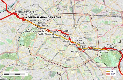
A comparative study of two transport lines known to be competing and complementary can provide the transport operator with valuable information. The study of the impact of multiple events on the use of transport lines could eventually help the operator to better anticipate a large influx of people to one line rather than the other. This case study can therefore be adapted to other such cases where transport lines partially follow a common route.

3.2. Data description

The daily inflow counts dataset was collected between 01/01/2011 and 07/31/2020 for two public transport lines (RER A and metro 1). These data were provided by the Paris public transport operator (Régie Autonome des Transports Parisiens, RATP). Figure 2 presents the daily counts and shows that there are more incoming flows to the RER line than to the metro line (40% more crowded when averaged over all days in the dataset).

Figure 2. Time series of daily inflow counts to RER A line and metro 1 line at ‘La Défense Grande Arche’ station for the time period 2011–2020.

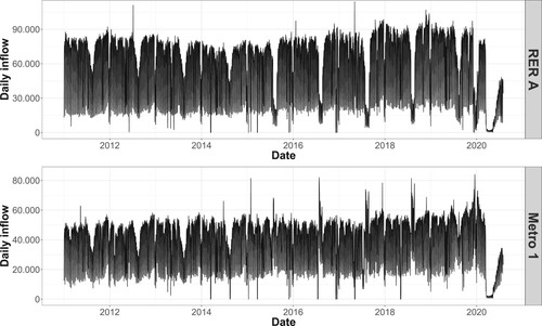
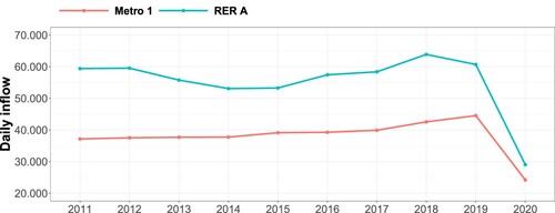
We can already have an idea of the underlying structures that govern the ridership time series by considering Figure 2. The average daily inflows per year are given by Figure 3. For the RER A the figure shows a long-term trend of decreasing ridership from 2012 to 2014, then an increasing trend from 2015 to 2018, and a decrease in 2019 and 2020. For metro 1, on the other hand, there is a constant increase in ridership except for 2020.

Figure 3. Daily inflow counts averaged per year to RER A line and metro 1 line at ‘La Défense Grande Arche’ station.

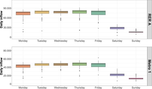
Two kinds of seasonalities can be seen in the ridership. First on a yearly scale, off-peak periods (vacations) and peak periods during the year are visible as can be seen in Figure 4 for the year 2011 which shows a typical pattern of yearly seasonality. Second on a weekly scale, weekdays have higher flows than weekend days. Indeed, a large number of workers commute to ‘La Défense’ hub daily, and about 85% of them use public transportation. This weekly seasonality is visible in Figure 5 where the medians, 1st and 3rd quartiles of ridership on the different days of the week were calculated over the year 2011. It is noteworthy that standard deviations are high, thus underlining a great diversity in the hub's temporal usage. These two phenomena of periodic variations of the ridership should be taken into account in the modeling as yearly and weekly seasonalities.

Figure 4. Time series of daily inflow counts to RER A line and metro 1 line at ‘La Défense Grande Arche’ station for the year 2011.

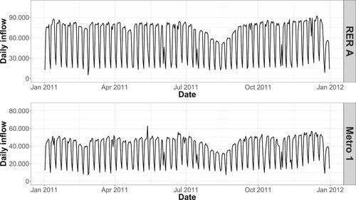
Figure 5. Boxplots of daily inflow counts for each day of the week over the year 2011 for RER A line and metro 1 line at ‘La Défense Grande Arche’ station.

These seasonal effects do not explain all the phenomena; the time series remain very noisy because they are subject to multiple external factors. Those listed in Table 1 are known to have an impact on daily ridership and were included in the models as explanatory variables. Most of these factors have been divided between working days and non-working days to account for the calendar effect. By non-working days we mean weekend days as well as bank holidays. On these days, there is very little work activity as opposed to working days, which are weekdays without bank holidays. We also consider maintenance events, strike days, and the health crisis period with the days of lockdown and post-lockdown. Finally we take into account the days when the urban transit system was free: during pollution peaks or car-free days; very few validation data were reported for these specific days.

Table 1. Exogenous variables included in the models.

Exogenous variables
Bank holidays
Extra days off
Summer maintenance work of the RER A on working days
Summer maintenance work of the RER A on non-working days
Maintenance work of metro 1 on working days
Maintenance work of metro 1 on non-working days
Transport operator strike days
Days of free travel on the transit network
Days of lockdown, Covid-19 period
Post-lockdown days, Covid-19 period

3.3. Application objectives

To the best of our knowledge, no studies have yet been conducted on the decomposition of time series applied to transit station ridership data. Considering the long time horizon over which the dataset was collected, it is interesting to decompose the time series to identify the impact of each exogenous factor on known or specific mobility behaviors (e.g. transfers). The transport operator provided us with nine-year ticketing data from two transport lines in the multimodal transport hub: RER A and metro 1. These lines are competing because they serve several stations in common but they are also complementary: the RER line serves more distant suburbs than the metro 1 line but the latter has a denser network of stations within Paris. One of the lines is automated (metro line 1), the other (RER line) is with a driver. A decomposition work on these time series will be an interesting case study. It will allow us to compare the effect of different exogenous factors, such as maintenance work or vacations, on the usage of these two competing lines. The temporal depth of our data will also allow us to examine two recent events that strongly impacted people's movements: the period of the strike against the pension reform in December 2019 and the period of the Covid-19 health crisis. This paper focuses on structural models of decomposition of daily station riderships captured by ticketing data. The first objective was to quantify the effect of various exogenous factors on use of the lines. The second objective was to compare these effects between two major and competing transport lines in the Paris region.

4. Description of the decomposition model structures

Each of the daily series describing the evolution of the number of passengers entering a transport line (RER A or metro 1) will be represented by the time series $(y_1,\dots ,y_n)$, where $y_t>0$ $(t=1,\dots ,n)$ is the number of people entering the line at day t, n being the number of observation days available. An additive structural model was chosen to represent the series $\log \left(y_t\right)$ (Equation (1(1) $\begin{array}{rl}\log \left(y_t\right)& =l_t+s_t+f_t+\sum _{j=1}^p{\text{β}}_t^{\left(j\right)}{X}_t^{\left(j\right)}+{\nu }_t,\end{array}$(1) )), which amounts to modeling the series $y_t$ in multiplicative form (Equation (2(2) $\begin{array}{rl}{y}_t& ={\mathrm{e}}^{l_t}\times {\mathrm{e}}^{s_t}\times {\mathrm{e}}^{f_t}\times \prod _{j=1}^p{\mathrm{e}}^{{\text{β}}_t^{\left(j\right)}{X}_t^{\left(j\right)}}\times {\mathrm{e}}^{{\nu }_t},\end{array}$(2) )). The logarithmic transformation has the advantage of forcing predictions of the number of passengers to remain positive while stabilizing the data variance (see Appendix 4). The model adopted is written as: (1) $\begin{array}{rl}\log \left(y_t\right)& =l_t+s_t+f_t+\sum _{j=1}^p{\text{β}}_t^{\left(j\right)}{X}_t^{\left(j\right)}+{\nu }_t,\end{array}$(1) (2) $\begin{array}{rl}{y}_t& ={\mathrm{e}}^{l_t}\times {\mathrm{e}}^{s_t}\times {\mathrm{e}}^{f_t}\times \prod _{j=1}^p{\mathrm{e}}^{{\text{β}}_t^{\left(j\right)}{X}_t^{\left(j\right)}}\times {\mathrm{e}}^{{\nu }_t},\end{array}$(2) where $l_t$ is the trend describing the long-term evolution of the series, $s_t$ is the weekly seasonal component, $f_t$ is the yearly seasonal component and ${\nu }_t$ is the residual component which is assumed to be distributed following a zero mean normal density, of variance ${\sigma }_{\nu }^2$. The model described by Equation (1(1) $\begin{array}{rl}\log \left(y_t\right)& =l_t+s_t+f_t+\sum _{j=1}^p{\text{β}}_t^{\left(j\right)}{X}_t^{\left(j\right)}+{\nu }_t,\end{array}$(1) ) also takes into account the dependence of data $y_t$ on p explanatory variables noted $(X_t^{\left(1\right)},\dots ,X_t^{\left(p\right)})$. Regression coefficients associated with these factors are noted $({\text{β}}_t^{\left(1\right)},\dots ,{\text{β}}_t^{\left(p\right)})$. Stochastic models describing each of the components of the model are explained below.

• The trend $l_t$ is a stochastic local level model defined as follows: (3) $l_t=l_{t-1}+b+{\omega }_t^l$(3) where b is a drift parameter and ${\omega }_t^l$ is white Gaussian noise.

• The weekly seasonal component $s_t$ is modeled in the stochastic form as follows: (4) $s_t=-\sum _{j=1}^6{s}_{t-j}+{\omega }_t^s,$(4) where ${\omega }_t^s$ is white Gaussian noise. This representation allows weekly seasonal patterns to evolve while ensuring that the sum of 7 consecutive terms of $s_t$ has a zero expected value.

• The yearly seasonal component is modeled in the following trigonometric form, which reduces the number of its parameters: (5) $\begin{array}{rl}{f}_t& =\sum _{u=1}^k{f}_{u,t}\end{array}$(5) (6) $\begin{array}{rl}{f}_{u,t}& =f_{u,t-1}\cos {\lambda }_u+f_{u,t-1}^{\ast }\sin {\lambda }_u+{\omega }_t^{f_u}\end{array}$(6) (7) $\begin{array}{rl}{f}_{u,t}^{\ast }& =-f_{u,t-1}\sin {\lambda }_u+f_{u,t-1}^{\ast }\cos {\lambda }_u+{\omega }_t^{f_u^{\ast }},\end{array}$(7) where ${\omega }_t^{f_u}$ and ${\omega }_t^{f_u\ast }$ are white Gaussian noises of the same variance. It is a combination of k stochastic cycles whose trigonometric representation is defined from the frequencies ${\lambda }_u=2\pi u/365$ for $u\in \{1,\dots ,k\}$.

• The regression coefficients associated with the exogenous variables $X_t^{\left(j\right)}$ are assumed to evolve following a Gaussian random walk defined by: (8) ${\text{β}}_t^{\left(j\right)}={\text{β}}_{t-1}^{\left(j\right)}+{\omega }_t^{{\text{β}}^{\left(j\right)}},$(8) where ${\omega }_t^{{\text{β}}^{\left(j\right)}}$ is a white Gaussian noise.

Note that for all components, all the residual terms are white Gaussian noise whose variances are summarized in Table 2. Initial values of components also follow Gaussian distributions whose parameters are specified in Table 2.

Table 2. Summary table of components parameters.

		Initial component parameters
Component	Variance	Expectation	Variance
Trend	${\sigma }_l^2$	$m_{l_0}$	$C_{l_0}$
(Equation (3(3) $l_t=l_{t-1}+b+{\omega }_t^l$(3) ))
Weekly seasonality	${\sigma }_s^2$	$m_{s_0}$	$C_{s_0}$
(Equation (4(4) $s_t=-\sum _{j=1}^6{s}_{t-j}+{\omega }_t^s,$(4) ))
Yearly seasonality	${\sigma }_{f_u}^2={\sigma }_{f_u^{\ast }}^2$	$m_{f_{u,0}}$	$C_{f_{u,0}}$
(Equations (6(6) $\begin{array}{rl}{f}_{u,t}& =f_{u,t-1}\cos {\lambda }_u+f_{u,t-1}^{\ast }\sin {\lambda }_u+{\omega }_t^{f_u}\end{array}$(6) ) and (7(7) $\begin{array}{rl}{f}_{u,t}^{\ast }& =-f_{u,t-1}\sin {\lambda }_u+f_{u,t-1}^{\ast }\cos {\lambda }_u+{\omega }_t^{f_u^{\ast }},\end{array}$(7) ))		$m_{f_{u,0}^{\ast }}$	$C_{f_{u,0}^{\ast }}$
Regression coefficients	${\sigma }_{{\text{β}}^{\left(j\right)}}^2$	$m_{{\text{β}}_0^{\left(j\right)}}$	$C_{{\text{β}}_0^{\left(j\right)}}$
(Equation (8(8) ${\text{β}}_t^{\left(j\right)}={\text{β}}_{t-1}^{\left(j\right)}+{\omega }_t^{{\text{β}}^{\left(j\right)}},$(8) ))
Residuals	${\sigma }_{\nu }^2$
(Equation (1(1) $\begin{array}{rl}\log \left(y_t\right)& =l_t+s_t+f_t+\sum _{j=1}^p{\text{β}}_t^{\left(j\right)}{X}_t^{\left(j\right)}+{\nu }_t,\end{array}$(1) ))

The term $\mathit{\theta }$ $=({\sigma }_l^2,{\sigma }_b^2,\dots .)$ will denote the set of unknown parameters of the model, described in Table 2, and ${\mathbf{x}}_t$ the vector of latent components of the model also known as state vector: ${\mathbf{x}}_t=(l_t,s_t,s_{t-1},\dots ,s_{t-6},f_{1,t},f_{1,t}^{\ast },\dots ,f_{k,t},f_{k,t}^{\ast },{\text{β}}_t^{\left(1\right)},\dots ,{\text{β}}_t^{\left(p\right)}{)}^T$Estimating the state vector ${\mathbf{x}}_t$, knowing the set of parameters $\mathit{\theta }$, is mainly based on the Kalman filter whose key steps are detailed in Appendix 1. The estimation of the unknown parameter $\mathit{\theta }$ can be achieved via different methods including maximum likelihood and quasi-Newton methods. For more details, the reader is referred to Appendix 1.

5. Results and discussion

In the calibration of the model, we aim to reduce its complexity while maintaining a satisfactory quality of data representation. We first selected which components should be considered and how they should be expressed in order to make sense of the decomposition. As some model parameters could not be deduced a priori, we used the AIC and RMSE criteria presented in Appendix 2 to choose them. Once the configuration was fixed, the parameters of the resulting model were estimated by the maximum likelihood method using the quasi-Newton method implemented by the BFGS algorithm (Appendix 1). We relied on the R toolbox dlm initiated by Petris (2010). The detailed calibration of the model is presented in Appendix 3. The model finally retained has deterministic yearly and weekly seasonalities. Its trend is constrained to keep only the long-term evolutions. It integrates covariates with a stochastic regression coefficient, and the yearly seasonality is based on a decomposition into six harmonics. The components estimated from the selected model are then analyzed. In our situation, the trend and the seasonal components were used to analyze natural variations in the station ridership, while components resulting from the explanatory variables were used to analyze the effect of anticipated periods (e.g. maintenance work on the metro/RER lines) and disturbances (e.g. strikes, Covid-19 health crisis).

The decomposition results are presented for each component: the state posterior expectation, and the 95% confidence interval calculated with the state posterior variance, for each day between 2011 and 2020. They are represented with solid black lines and grey filled areas respectively on the figures in Sections 5.1–5.4. Components were log scaled, in particular, to visualize confidence intervals better. For some components it will be important to differentiate working days from non-working days that will be represented with red and blue dots respectively (in Sections 5.2–5.4). The exponential transformation of the regression coefficients ${\mathrm{e}}^{{\text{β}}_t^{\left(s\right)}}$ of each exogenous variable s made it possible to quantify the impact of each variable on the transport line ridership. For a given day t, variable s multiplies the ridership by the value ${\mathrm{e}}^{{\text{β}}_t^{\left(s\right)}}$ in relation to a reference level of ridership. For example, take the effect of the variable $s=$ ‘Maintenance work days on RER line’ which has the value ${\mathrm{e}}^{{\text{β}}_t^{\left(s\right)}}=0.7$ on a given day: this implies that maintenance work days impact ridership and explains why there is only 70% ridership.

5.1. The natural variations in station ridership

Figure 6 (metro) and Figure 7 (RER) present the original patterns of transport ridership time series as well as the trend and the seasonality components.

Figure 6. Decomposition of the time series of flows entering the metro line ($y_t$) into log-scaled trend ($l_t$), log-scaled annual seasonality ($f_t$), and log-scaled residuals (${\nu }_t$) (left panel).

Log-scaled annual profile of the $f_t$ component with the different vacation periods in blue and enlargement over four weeks of log-scaled weekly seasonality $s_t$ (right panel)

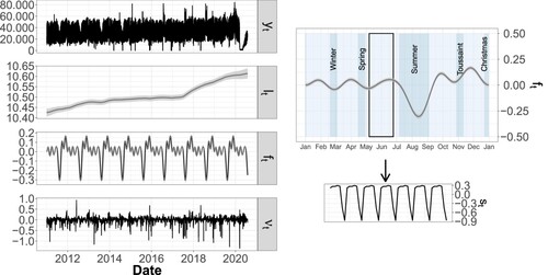
Figure 7. Decomposition of the time series of flows entering the RER line ($y_t$) into log-scaled trend ($l_t$), log-scaled annual seasonality ($f_t$), and log-scaled residuals (${\nu }_t$) (left panel).

Log-scaled annual profile of the $f_t$ component with the different vacation periods in blue and enlargement over four weeks of log-scaled weekly seasonality $s_t$ (right panel).

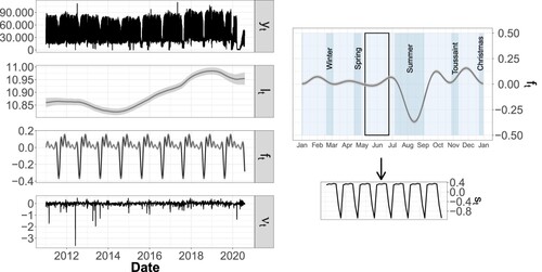
Trends of changes in ridership over the years show differences between the two transport lines. For the metro (see Figure 6), we note an increase in ridership over the years, with an acceleration starting in 2017. This can be explained by the rise in traffic on the east-west Parisian axis, induced by an increasing concentration of jobs in the west, particularly in the ‘La Défense’ district. For the RER (see Figure 7), the trend $l_t$ shows a profile that is more difficult to interpret as it declines between 2011 and 2014, unlike the metro. We link this decrease to the creation of two new exits from a tramway line adjacent to the RER line after 2012, which no doubt modified the movement dynamics in the whole western part of the exchange pole. The increase that follows is in line with the dynamics observed in the metro. The decrease in this component, as well as the increase in its uncertainty during the period from the end of 2019 to the year 2020, are attributable to the impacting events of strikes and the COVID-19 pandemic.

The two transport lines show similar yearly seasonal components $f_t$. The significant troughs between July and October correspond to the summer vacation periods associated with a considerable drop in station ridership (${\mathrm{e}}^{f_t}=0.67$ for RER and 0.74 for metro). The summer vacations are responsible for a decrease of nearly 30% in the number of visitors for the two lines. The other school holidays (winter, spring, autumn, and Christmas) are also apparent. Note the presence of over-crowding periods just before the Christmas vacations. There is, however, a difference between the two profiles during the first part of each year, before the summer vacations: metro line ridership fluctuates more between holiday and work periods than RER line ridership, which remains more constant. The uncertainty is higher during summer vacations than during the rest of the year. As we will see later, maintenance work often occurs at these times, significantly modifying the ridership from one year to the next.

The weekly seasonal components $s_t$ are difficult to visualize with this scale. We therefore present a comparative magnification of the two profiles in Figure 8. The weekly seasonal component coefficients ${\mathrm{e}}^{s_t}$ associate each day of the week with a percentage of ridership relative to a reference level. They thus reflect the level of ridership on each of these days. The profiles between the two transport lines are very similar with high weights allocated to weekdays (${\mathrm{e}}^{{\text{β}}_t^{\left(s\right)}}>1.2$, ridership 20% higher than a reference level) and low weights assigned to the weekend (ridership around 60% of the reference level on Saturdays and 40% on Sundays). A slight difference can be observed between weekdays with known patterns in public transport: Mondays are slightly less busy, and there is also a small decrease on Wednesdays (a day without school for some children). Tuesdays and Thursdays attract more people. Note that there seem to be more significant differences between weekdays and weekends for the RER than for the metro.

Figure 8. Log-scaled weekly seasonality $s_t$ and 95% confidence intervals for flows entering the RER line (purple) and the metro line (green).

Residuals ${\nu }_t$ allow us to detect days when the model has not, or wrongly, taken an effect into account. For the two transport lines, we note that some days with unanticipated transport breakdowns or events requiring the closure of lines for a large part of the day are associated with large residuals. For example, September 21, 2019 has a large residual because a demonstration prevented the arrival of the metro at the ‘La Défense Grande Arche’ station.

5.2. Analysis of the impact of maintenance work

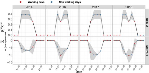
Maintenance work has a strong impact on the ridership dynamics of the transport hub. It can cause flow decreases or transfers. Beginning with the RER line maintenance work periods: each summer since 2015, it has been subject to work that requires the line to be shut down during weekdays and/or weekends. To visualize the effect of this maintenance work, we will represent the regression coefficients of maintenance work multiplied by the associated class indicators. Results are shown in Figure 9 for the impact of work on RER line ridership and in Figure 10 for the metro line.

Figure 9. Log-scaled component associated with maintenance work on the RER line and 95% confidence interval for incoming flows in the RER line. Summers between 2015 and 2020 are represented.

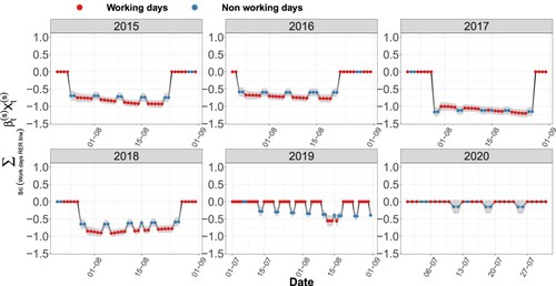
Figure 10. Log-scaled component associated with maintenance work on the RER line and 95% confidence interval for incoming flows in the metro line. Summers between 2015 and 2020 are represented.

These results reveal notable differences between the two transport lines: while the impact is strongly negative on RER line ridership, the opposite is true for the metro line. This result underlines the importance of metro line 1 as a substitute for RER line A to cross Paris.

The impact of maintenance work on the use of the RER line is not total; it falls to a minimum of ${\mathrm{e}}^{{\text{β}}_t^{\left(s\right)}}=0.3$ in 2017. As ‘La Défense Grande Arche’ is an interchange station, flows of people can continue to transit through the access area to the RER line to reach other lines; the drop nevertheless underlines that most people no longer transit through this area. Furthermore, note the lesser importance of work on the RER line ridership decrease during the 2019 and 2020 summers compared to other summers (Figure 9). During these two summers, maintenance work only took place on weekends (except for the week of the 15th August in 2019 with maintenance work every day). We make two assumptions to explain this phenomenon:

• Since the work took place every day from 2015 to 2018, more people chose to go on vacation during the summer or shifted to another transportation mode (e.g. car).

• The work took place between the transport hub and Paris from 2015 to 2018 and then within Paris itself in 2019 and 2020: an alternative to metro line 1 was possible for the inhabitants of eastern Paris wishing to go to ‘La Défense’ in 2019 and 2020. This can be seen from the regression coefficients for the metro, which are lower in 2019 and 2020 than in other years.

Like the RER line, the metro line is sometimes shut down because of maintenance work. Figure 11 shows the regression coefficients associated with this effect. Maintenance work on the metro line had a considerable impact on metro line ridership. Unlike the access area to the RER line, the metro line area is not a transfer area, and almost no one comes in when the line is stopped. Similarly, as for maintenance work on the RER line, we note a flow transfer phenomenon, this time from the metro to the RER line whose use increased slightly.

Figure 11. Log-scaled component associated with maintenance work on the metro line and 95% confidence interval for incoming flows in the RER and metro lines.

On the different charts, large confidence intervals are associated with the effects on the metro line. Due to the few days of maintenance work on the metro line, the uncertainty is significant. In particular, the impact of the work is very variable over the few days on which it takes place.

5.3. Strike periods: analysis of the case of the long strike of December 2019–January 2020

The period from December 2019 to January 2020 was characterized by a massive mobilization against the reform of the French pension system. Support for the strike was very strong at the RATP transport operator, severely disrupting its entire public transportation network. Comparison of the impact of this strike on the riderships of the two lines is visualized in Figure 12.

Figure 12. Log-scaled components associated with strike effect and 95% confidence intervals for incoming flows in RER and metro lines for the period from December 2019 to January 2020.

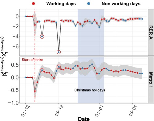
The study of these profiles shows that while the effect of the strike was negative for RER line ridership, it was positive for the metro line from December 7. This phenomenon is due to a transfer of flows from the RER line to the metro line. The metro is an automatic metro line that maintained normal service during the strike, while the RER traffic was severely disrupted. This phenomenon also led to numerous situations of congestion and overloading of the metro. RER traffic improved after the Christmas holidays. In Figure 12, we have framed the Christmas holidays period, which separates two trends:

• Before the vacation: The first weeks of the strike were particularly difficult for RER traffic. The strike had a very marked effect on RER traffic, as it explains a decrease of more than half in RER line ridership (${\mathrm{e}}^{{\text{β}}_t^{\left(s\right)}}$ coefficient below 0.5). On the other hand, passenger flows at the metro line increased steadily: the coefficient increases from ${\mathrm{e}}^{{\text{β}}_t^{\left(s\right)}}=1$ on the 3rd day of the strike to more than 1.5 at the beginning of the vacation. As the strike progressed, while the RER traffic was severely disrupted, the effect of the transfer to the metro line was increasingly significant, to the point of overloading the line by more than 50% above reference use.

• After the vacation: As the situation improved for RER traffic, there was a gradual return to a normal RER and metro line ridership situation.

Note the presence of the two Sundays December 8 and 15 (circled in red in Figure 12) during which there was almost no use of the RER line: the RER traffic was indeed wholly cut off on those days. Uncertainty remained practically constant throughout the period, except for Christmas Day and New Year's Day: the cumulative effect of these particular days and the strike makes the estimation of the strike's impact more uncertain.

5.4. Lockdown and post-lockdown periods related to the Covid-19 pandemic

The public transport sector was heavily impacted by the Covid-19 pandemic, making it a key case study. Gkiotsalitis and Cats (2020) proposed a network-wide model that can set the optimal frequency of transport lines under different distancing scenarios. The lockdown period due to the Covid-19 pandemic had, unsurprisingly, a considerable impact on the use of the transport hub. Most of the office workers who travel daily to ‘La Défense’ could not go to work during this period because of the lockdown. The post-lockdown period also significantly impacted the hub usage since telecommuting was strongly recommended. Here more than anywhere else, the Covid-19 pandemic period had a decisive effect on travel habits. We present the regression coefficients associated with the periods of lockdown and post-lockdown in Figure 13.

Figure 13. Log-scaled components associated with lockdown/post-lockdown periods and 95% confidence interval for incoming flows in RER and metro lines.

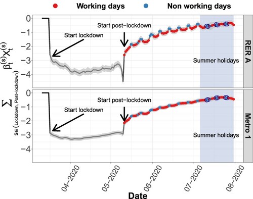
For both transport lines (see Figure 13), there is an effect of the almost total loss of ridership during the lockdown period from March 17, 2020, to May 11, 2020. The ${\text{β}}_t^{\left(s\right)}$ coefficient is around -3 during this period and thus ${\mathrm{e}}^{{\text{β}}_t^{\left(s\right)}}$ around zero. There is no noticeable difference between weekdays and weekends: no one was present at the access to the lines on any day. We note an odd behavior that maximizes the lockdown effect the day before post-lockdown for the RER.

The impact of the post-lockdown period (from May 11th), which is very visible in Figure 13, shows similarities and differences between the two lines. First of all, there is, for both cases, a slow return to a normal situation with a surprising wave profile: post-lockdown had a stronger effect on the decrease in ridership on weekdays than on weekend days. While this effect is visible in both cases, it is more pronounced for the RER line than for the metro. In addition to being a place of work, 'La Défense' is also a major shopping center in the Parisian region. Companies maintained pressure to keep telecommuting beyond legal post-lockdown. There may have been a stronger psychological acceptability of taking risks for shopping and individual leisure activities than for work.

We assume that, while this period of social distancing resulted in a strong incentive to adopt telecommuting, the impacts on weekend habits, i.e. shopping in this case, are different. Since the RER suburban train connects the ‘La Défense’ hub to more suburbs than metro line 1, it affects more people, making this hypothetical effect more visible on the RER line ridership than on the metro one. We frame the summer vacation period, which seemed to completely suppress the wave profile of a return to normal. Uncertainty also increased during this period. The vacation period completely changed the return-to-normal profile, no doubt due to the fact that during the summer vacation, the RER line was under maintenance work on weekends (circled in blue in Figure 13). The phenomenon of declining use of stations can therefore be explained by two variables: post-lockdown period and maintenance work. For this reason, uncertainty also increased during the summer vacation.

6. Conclusion

This paper has presented the analysis of ticketing data collected at several control points of a multimodal transportation hub, each serving access to a transport line, based on structural models of time series decomposition. We focused our analysis on daily ridership collected over nine years. The strength of such models lies in their explanatory capacity. They are capable of highlighting long-term phenomena on the ridership, such as the trend and seasonality (annual, weekly) and the impact of exogenous factors, whether anticipated, such as maintenance work or not, such as strikes or the Covid-19 health crisis. Through the regression coefficients of the decomposition model, we can quantify this impact separately for each factor, which is impossible with other learning-based models. These models also allow us to predict daily ridership over several time horizons. Since both transit lines serve the same transit stations, the decomposition was able to identify and quantify some modal shifts between the two lines, particularly during periods of maintenance work. In this article, we have addressed all the questions relating to the estimation of these models' parameters, in order to obtain a decomposition appropriate to the data under consideration. However, despite their strong descriptive aspect, structural time series models require fine calibration and extensive statistical knowledge. Moreover, it is necessary to succeed in combining business knowledge with modeling choices. Some practical cases that can use this type of work may concern feedback on the impact of typical events such as maintenance work or strikes.

Several extensions to this work are to be expected. It will be interesting to work at a shorter time-scale, to study events with well-localized effects, such as concerts or evening work. The extension to multivariate time series is also a relevant continuation of this work. A multivariate model considering several mobility data would implicitly introduce a covariance structure between the error terms of the different time series, thus providing us with correlation information between the errors of several series. Another avenue of work would be to combine this type of model with machine learning models to predict or detect anomalies over short or medium-term time horizons. the fine analysis of residuals can also allow the detection of outliers A transferability of this work to other case studies is possible due to the adaptability of these models. For this reason we make available the source code for the analyzes with the dlm package at https://github.com/pdenailly/TransportHub_TimeSeriesDecomposition.

Disclosure statement

No potential conflict of interest was reported by the author(s).

Appendices

Appendix 1.

Model estimation

Kalman filter allows to estimate the state vector ${\mathbf{x}}_t$, given the parameters $\mathit{\theta }$. Detailed formulas can be found in Shumway and Stoffer (1982). Three estimation stages are generally used in this framework: prediction, filtering, and smoothing. Noting ${\mathbf{x}}_t^s$ the expectation of ${\mathbf{x}}_t$ conditionally to observed data up to time s and ${\mathbf{P}}_t^s$ the covariance matrix of ${\mathbf{x}}_t$ conditionally to observed data up to time s, the prediction, filtering and smoothing steps are defined as follows:

• The prediction step consists in evaluating ${\mathbf{x}}_t^{t-1}$ and ${\mathbf{P}}_t^{t-1}$ based on ${\mathbf{x}}_{t-1}^{t-1}$ and ${\mathbf{P}}_{t-1}^{t-1}$.

• The filtering step consists in evaluating ${\mathbf{x}}_t^t$ and ${\mathbf{P}}_t^t$ based on the current observation $\log \left(y_t\right)$ and the quantities ${\mathbf{x}}_t^{t-1}$ and ${\mathbf{P}}_t^{t-1}$. It is a matter of correcting the predictions obtained in the previous step, using this new available information. Kalman filter generally refers to the iterated prediction and filtering steps for $t=1,\dots ,n$.

• The purpose of the smoothing step is to calculate ${\mathbf{x}}_t^n$ and ${\mathbf{P}}_t^n$ knowing all the data. These two quantities are recursively obtained for $t=n,\dots ,1$.

Several methods can be used to estimate state space model parameters. One example is the expectation-maximization (EM) algorithm, originally developed by Dempster, Laird, and Rubin (1977) and then exploited by Shumway and Stoffer (1982) for the estimation of linear state space model parameters. For our model, the EM algorithm aims at maximizing log-likelihood with respect to all parameters $\mathit{\theta }$. The algorithm iterates two steps until convergence: a step to estimate smoothed components ${\mathbf{x}}_t^n$ knowing the parameters and a parameter update step knowing the smoothed components.

Another parameter estimation method used in the state space models framework is the quasi-Newton method implemented in the BFGS algorithm, which is based on a gradient projection and on the approximation of the hessian matrix of log-likelihood by a matrix with limited memory (Byrd et al. 1995). This was the method chosen in the present study as convergence is generally faster than with the EM algorithm and restrictions on parameter spaces are accepted (Petris, Petrone, and Campagnoli 2009).

Appendix 2.

Criteria for comparing models

To evaluate different models so as to select the best one, we based our work on two criteria:

• The Akaike information criterion or AIC (Akaike 1974), defined by (A1) $AIC=-2L+2\kappa ,$(A1) where L is the model log-likelihood and κ the number of estimated parameters. Note that the best model is the one minimizing the AIC criterion.

• The root mean square error between observations and forecasts (RMSE), evaluated on a test sample for different forecasting horizons $h\ge 1$: (A2) $RMSE\left(h\right)=\sqrt{\sum _{i=1}^{n-h}\frac{\left({\hat{y}}_{i+h}\right(i)-y_{i+h}{)}^2}{n-h}},$(A2) where ${\hat{y}}_{i+h}\left(i\right)$ is the forecast of $y_{i+h}$ obtained from observations $(y_1,\dots ,y_i)$.

Appendix 3.

Model calibration

The model should give priority to the descriptive aspect rather than the predictive one to make as much sense as possible of the decomposition; a preference for deterministic components will materialize this point. To determine a suitable model for our data, we first specified some a priori knowledge about the configuration it should take. This is first of all, the choice of which components should be included in the model. In Section 3.2 we determined that long-term trends, weekly and yearly seasonalities seemed to explain a large part of the variations in ridership and some possible exogenous factors. More specifically, we look for a model with a slow evolution of trends, deterministic and stable seasonal components in which there is little variability. Some exogenous effects should also be added, with the possibility of varying in intensity to quantify their impact at different periods. These choices are formalized in the components as follows:

• Trend

  To ensure that the trend (Equation (3(3) $l_t=l_{t-1}+b+{\omega }_t^l$(3) )) only reflects changes in ridership over the long term (9 years), we constrained the trend's variance not to exceed an upper bound ($<3\times {10}^{-7}$).

• Weekly seasonality

  To better visualize the effect of the different days of the week on station ridership, we chose a deterministic component that does not contain stochastic modifications (${\omega }_t^s=0$).

• Yearly seasonality

  Similarly to the weekly seasonal component, we opted for a deterministic yearly component. Variances ${\sigma }_{{\omega }^{f_u}}^2$ and ${\sigma }_{{\omega }^{f_u^{\ast }}}^2$ of the error terms were set to zero so that the two errors ${\omega }_t^{f_u}$ and ${\omega }_t^{f_u^{\ast }}$ are zero (see Equations (5(5) $\begin{array}{rl}{f}_t& =\sum _{u=1}^k{f}_{u,t}\end{array}$(5) ) to (7(7) $\begin{array}{rl}{f}_{u,t}^{\ast }& =-f_{u,t-1}\sin {\lambda }_u+f_{u,t-1}^{\ast }\cos {\lambda }_u+{\omega }_t^{f_u^{\ast }},\end{array}$(7) )). The objective here was to highlight the variations in ridership, on average, over a year.

• Regression coefficients

  The effect of exogenous factors should be allowed to vary over time to take account of their temporal evolution. Thus, no constraint was imposed on the parameters ${\sigma }_{{\text{β}}^{\left(j\right)}}^2$ of this component.

The number of harmonics in the annual seasonal component is not a parameter that can be calibrated a priori, so this choice will be made on the basis of the AIC (Akaike 1974) and RMSE metrics.

Considering the constraints described above, several model configurations were compared for the two transport lines: the absence of an annual seasonal component (k = 0) and the number of harmonics k varying overall $2,4,6,8,10,12$. These different models were tested with and without the presence of explanatory variables. The choice of the number of harmonics was based on the minimization of the AIC criterion evaluated over the learning period (years 2011–2015), and the RMSE calculated on the test basis (years 2016 and 2017) both described in Appendix B1. The criteria obtained for each of the considered configurations are given in Table A1 and Figure A1.

Figure A1. RMSE criterion obtained for different configurations of the model over the years 2016 and 2017 by varying the h forecast horizon from 1 to 7.

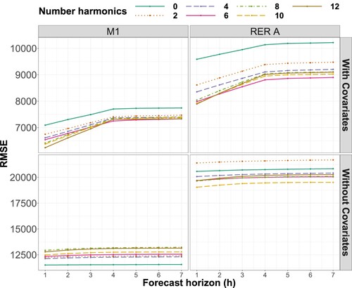
Table D1. AIC criterion obtained for different configurations of the model: number of harmonics (yearly component), presence or absence of covariates.

		AIC
Transport line	Harmonics	Without covariates	With covariates
	0	836	−3880
	2	822	−4108
	4	800	−4280
RER A	6	766	−4430
	8	762	−4504
	10	754	−4514
	12	750	−4540
	0	942	−4262
	2	930	−4634
	4	916	−4846
Metro 1	6	900	−4994
	8	874	−5122
	10	872	−5158
	12	872	−5168

Table A1 shows that the AIC criterion is better when the number of harmonics increases. This result is consistent because the number of parameters to be estimated does not increase when the number of harmonics of the annual component is increased, but the likelihood does. The AIC criterion obtained from models with covariates is better than that obtained from models without covariates. Between models with 10 and 12 harmonics, there is no significant improvement in the AIC criterion. The RMSE criterion is more interesting here to distinguish between the models. As expected, the increase in the prediction horizon h leads to an increase in the prediction error. Models with covariates improve prediction performance. Several observations emerge from Figure A1:

• For models without exogenous variables, the choice of ten harmonics is better for the RER data, and the model without the annual component is better for metro data. While an annual component capable of capturing peak and off-peak periods is a good addition to the first case model, it is penalizing in the second case. The 2017 and 2018 summer ridership profiles are totally modified due to RER line maintenance work.

• For models with exogenous variables, despite close prediction capabilities between the different models, versions with k = 6 harmonics seem to be slightly better than the others for both transport lines (Metro 1 for $\mathrm{h}=4$, 5, 6, 7 and RER A for $\mathrm{h}=2$, 3, 4, 5, 6, 7).

Appendix 4.

Choice of model type between additive and multiplicative

The aim of this appendix is to compare multiplicative (Equation (A3(A3) $\begin{array}{rl}\log \left(y_t\right)& =l_t+s_t+f_t+\sum _{j=1}^p{\text{β}}_t^{\left(j\right)}{X}_t^{\left(j\right)}+{\nu }_t,\end{array}$(A3) )) and additive (Equation (A4(A4) $\begin{array}{rl}{y}_t& =l_t+s_t+f_t+\sum _{j=1}^p{\text{β}}_t^{\left(j\right)}{X}_t^{\left(j\right)}+{\nu }_t,\end{array}$(A4) )) decomposition models in order to select the model that is most suitable to explain our flow data. (A3) $\begin{array}{rl}\log \left(y_t\right)& =l_t+s_t+f_t+\sum _{j=1}^p{\text{β}}_t^{\left(j\right)}{X}_t^{\left(j\right)}+{\nu }_t,\end{array}$(A3) (A4) $\begin{array}{rl}{y}_t& =l_t+s_t+f_t+\sum _{j=1}^p{\text{β}}_t^{\left(j\right)}{X}_t^{\left(j\right)}+{\nu }_t,\end{array}$(A4) There are two ways to decide between the two types of models:

• Empirical observations

  The multiplicative model can deal with the cumulative effect of several components that negatively affect the flows, while an additive model can theoretically consider component accumulations as negative. This is what we have observed by visualizing one-step predictions made with the two forms of models. For example, let's take August 2017, where a bank holiday occurred on August 15, during the summer holidays. Figure A2 shows the incoming traffic in the RER A station and the predictions made by the two models. It can be seen that the additive model considers a very strong effect which, when combined with the summer holiday effect, leads to a distorted prediction during the bank holiday.

• Comparisons between predictive capabilities

  These two models are compared based on their predictive capacities over several time horizons. To do this, we used the notion of RMSE per forecast horizon (see Appendix 2). Learning periods covered the years 2011–2015, and the test basis was the year 2016. The results are presented in Figure A3. The multiplicative model provides better predictions for the RER A daily inflows than the additive model, whatever the forecast horizon (h). This result is less pronounced for metro 1, where the multiplicative model is only better for predictions at $\mathrm{h}=4$ to $\mathrm{h}=7$. In this case, summer maintenance work was carried out. At small forecast horizons, the Kalman algorithm's filtering phase has more difficulty correcting the components in the case of log data of the multiplicative model than in the case of non-log data of the additive model when the maintenance period is encountered. At larger forecast horizons, the difference disappears because the components had more time to adapt to the change.

Figure A2. Observed and one-day ahead predicted daily inflows of people to the RER A line at La Défense Grande Arche station. Observed counts are in black, predictions made with the additive model in red, and predictions made with the multiplicative model in purple.

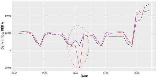
Figure A3. RMSE(h) errors calculated for forecast horizon (h) ranging from 1 to 7 over the year 2016 for the additive and multiplicative models applied to daily inflows to RER A (top) and Metro 1 (bottom).

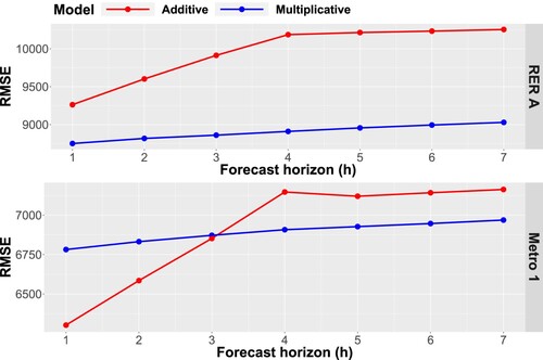
We chose the multiplicative model for our series decomposition. This model has the advantage over the additive model of forcing observed values to remain positive, and its prediction capacities are close to those of the additive model.

References

- Akaike, Hirotugu. 1974. “A New Look at the Statistical Model Identification.” IEEE Transactions on Automatic Control 19 (6): 716–723.
- Almannaa, Mohammed H., Mohammed Elhenawy, and Hesham A. Rakha. 2020. “Dynamic Linear Models to Predict Bike Availability in a Bike Sharing System.” International Journal of Sustainable Transportation 14 (3): 232–242.
- Bagchi, Mousumi, and Peter R. White. 2004. “What Role for Smart-Card Data From Bus Systems?” In Proceedings of the Institution of Civil Engineers-Municipal Engineer, Vol. 157, No. 1, 39–46. Thomas Telford Ltd.
- Bian, Zheyong, Zhipeng Zhang, Xiang Liu, and Xiao Qin. 2019. “Unobserved Component Model for Predicting Monthly Traffic Volume.” Journal of Transportation Engineering, Part A: Systems 145 (12): Article ID 04019052.
- Borgnat, Pierre, Etienne Come, and Latifa Oukhellou. 2017. “Processing, Mining and Visualizing Massive Urban Data.” In ESANN 2017 Proceedings, European Symposium on Artificial Neural Networks, Computational Intelligence and Machine Learning, Bruges (Belgium), 26–28 April 2017.
- Briand, Anne-Sarah, Etienne Côme, K. Mohamed, and Latifa Oukhellou. 2016. “A Mixture Model Clustering Approach for Temporal Passenger Pattern Characterization in Public Transport.” International Journal of Data Science and Analytics 1 (1): 37–50.
- Byrd, Richard H., Peihuang Lu, Jorge Nocedal, and Ciyou Zhu. 1995. “A Limited Memory Algorithm for Bound Constrained Optimisation.” SIAM Journal on Scientific Computing 16 (5): 1190–1208.
- Chen, Jason Li, Gang Li, Doris Chenguang Wu, and Shujie Shen. 2019. “Forecasting Seasonal Tourism Demand Using a Multiseries Structural Time Series Method.” Journal of Travel Research 58 (1): 92–103.
- Cui, Chunsheng, Hongfei Jia, Liping Huang, and Xiaopeng Zhang. 2016. “Fuzzy Multivariate Narx Model for Passenger Entrance Flow Prediction in the Shanghai Subway System.” Journal of Intelligent & Fuzzy Systems 31 (6): 3047–3054.
- Dempster, Arthur P., Nan M. Laird, and Donald B. Rubin. 1977. “Maximum Likelihood From Incomplete Data Via the EM Algorithm.” Journal of the Royal Statistical Society: Series B (Methodological) 39 (1): 1–22.
- Doorley, Ronan, Vikram Pakrashi, Brian Caulfield, and Bidisha Ghosh. 2014. “Short-Term Forecasting of Bicycle Traffic Using Structural Time Series Models.” In 17th International IEEE Conference on Intelligent Transportation Systems (ITSC), 1764–1769. IEEE.
- Dordonnat, V., Siem Jan Koopman, Marius Ooms, A. Dessertaine, and J. Collet. 2008. “An Hourly Periodic State Space Model for Modelling French National Electricity Load.” International Journal of Forecasting 24 (4): 566–587.
- El Mahrsi, Mohamed K., Etienne Côme, Latifa Oukhellou, and Michel Verleysen. 2016. “Clustering Smart Card Data for Urban Mobility Analysis.” IEEE Transactions on Intelligent Transportation Systems 18 (3): 712–728.
- Ghosh, Bidisha, Biswajit Basu, and Margaret O'Mahony. 2009. “Multivariate Short-Term Traffic Flow Forecasting Using Time-Series Analysis.” IEEE Transactions on Intelligent Transportation Systems 10 (2): 246–254.
- Gkiotsalitis, Konstantinos, and Oded Cats. 2020. “Optimal Frequency Setting of Metro Services in the Age of COVID-19 Distancing Measures.” Preprint, arXiv:2006.05688.
- Grieser, Jürgen, Silke Trömel, and C.-D. Schönwiese. 2002. “Statistical Time Series Decomposition Into Significant Components and Application to European Temperature.” Theoretical and Applied Climatology 71 (3–4): 171–183.
- Harvey, Andrew C. 1990. Forecasting, Structural Time Series Models and the Kalman Filter. Cambridge university press, Cambridge, UK.
- He, Li, Bruno Agard, and Martin Trépanier. 2020. “A Classification of Public Transit Users with Smart Card Data Based on Time Series Distance Metrics and a Hierarchical Clustering Method.” Transportmetrica A: Transport Science 16 (1): 56–75.
- Honjo, Keita, Hiroto Shiraki, and Shuichi Ashina. 2018. “Dynamic Linear Modeling of Monthly Electricity Demand in Japan: Time Variation of Electricity Conservation Effect.” PloS One 13 (4): Article ID e0196331.
- Koopman, Siem Jan, and Marius Ooms. 2011. “Forecasting Economic Time Series Using Unobserved Components Time Series Models” in The Oxford Handbook of Economic Forecasting, M. P. Clements and D. F. Hendry, Eds, Oxford University Press, Oxford.
- Lathia, Neal, Chris Smith, Jon Froehlich, and Licia Capra. 2013. “Individuals Among Commuters: Building Personalised Transport Information Services From Fare Collection Systems.” Pervasive and Mobile Computing 9 (5): 643–664.
- Lisi, Francesco, and Matteo Pelagatti. 2016. “Component Estimation for Electricity Market Data: Deterministic Or Stochastic?.” Energy Economics 74: 13–37.
- Luo, Ding, Oded Cats, and Hans van Lint. 2017. “Analysis of Network-Wide Transit Passenger Flows Based on Principal Component Analysis.” In 5th IEEE International Conference on Models and Technologies for Intelligent Transportation Systems (MT-ITS), 744–749. IEEE.
- Marczak, Martyna, and Tommaso Proietti. 2016. “Outlier Detection in Structural Time Series Models: The Indicator Saturation Approach.” International Journal of Forecasting 32 (1): 180–202.
- Mousavi, Mir Hossein, and Saleh Ghavidel. 2019. “Structural Time Series Model for Energy Demand in Iran's Transportation Sector.” Case Studies on Transport Policy 7 (2): 423–432.
- Murthy, K. V. Narasimha, and G. Kishore Kumar. 2020. “Structural Time-Series Modelling for Seasonal Surface Air Temperature Patterns in India 1951–2016.” Meteorology and Atmospheric Physics 133 (1): 27–39.
- Murthy, K. V. Narasimha, R. Saravana, and P. Rajendra. 2019. “Unobserved Component Modeling for Seasonal Rainfall Patterns in Rayalaseema Region, India 1951–2015.” Meteorology and Atmospheric Physics 131 (5): 1387–1399.
- Petris, Giovanni. 2010. “An R Package for Dynamic Linear Models.” Journal of Statistical Software 36 (12): 1–16.
- Petris, Giovanni, Sonia Petrone, and Patrizia Campagnoli. 2009. “Dynamic Linear Models.” In Dynamic Linear Models with R, 31–84. New York, NY: Springer.
- Poussevin, Mickaël, Emeric Tonnelier, Nicolas Baskiotis, Vincent Guigue, and Patrick Gallinari. 2015. “Mining Ticketing Logs for Usage Characterization with Nonnegative Matrix Factorization.” In Big Data Analytics in the Social and Ubiquitous Context, 147–164. Cham: Springer.
- Rodriguez, Yesid, Wilmer Pineda, and Oscar Diaz Olariaga. 2020. “Air Traffic Forecast in Post-Liberalization Context: A Dynamic Linear Models Approach.” Aviation 24 (1): 10–19.
- Roos, Jérémy, Stephane Bonnevay, and Gérald Gavin. 2016. “Short-Term Urban Rail Passenger Flow Forecasting: A Dynamic Bayesian Network Approach.” In 15th IEEE International Conference on Machine Learning and Applications (ICMLA), 1034–1039. IEEE.
- Shumway, Robert H., and David S. Stoffer. 1982. “An Approach to Time Series Smoothing and Forecasting Using the EM Algorithm.” Journal of Time Series Analysis 3 (4): 253–264.
- Shumway, Robert H., and David S. Stoffer. 2000. Time Series Analysis and Its Applications. Vol. 3. New York: Springer.
- Toqué, Florian, Etienne Côme, Martin Trépanier, and Latifa Oukhellou. 2020. “Forecasting of the Montreal Subway Smart Card Entry Logs with Event Data.” Preprint, arXiv:2008.09842.
- Zhang, Jinlei, Feng Chen, Yinan Guo, and Xiaohong Li. 2020. “Multi-Graph Convolutional Network for Short-Term Passenger Flow Forecasting in Urban Rail Transit.” IET Intelligent Transport Systems 14 (10): 1210–1217.
- Zhu, Xi, and Diansheng Guo. 2017. “Urban Event Detection with Big Data of Taxi OD Trips: A Time Series Decomposition Approach.” Transactions in GIS 21 (3): 560–574.