Public transport path choice estimation based on trip data from dedicated smartphone app survey

Abstract

Having access to realistic and empirically grounded passenger valuations of public transport trip components facilitate the undertaking of necessary trade-offs during planning of transport networks. Discrete choice estimation of path choice preferences is a practical way to obtain such preferences. This paper proposes a new take on the empirical foundation of path choice estimation based on revealed choices by introducing trip data for full activity-based ‘door-to-door’ public transport trips collected from a dedicated survey application for smartphones. Choice probabilities were modelled based on an explicitly generated choice set, where the public transport trip parts were generated using a branch-and-bound approach. Results in terms of estimated preferences are comparable to those based on conventional surveying methods and suggest significant premiums for paths involving public transport stops with an elevated level of passenger service as well as differences in preferences across population groups.

KEYWORDS:

• Public transport
• path choice
• discrete choice model

1. Introduction

Abundant initiatives in many metropolitan areas to mitigate traffic congestion and ensure accessibility for all, given growing populations and increased clustering of residents and workplaces, endorse the case for efficient urban mass transportation (Florida 2018), also known as public transport (PT). Due to resource limitations in of PT planning and operation organisations, the ability to design and optimise the PT network is crucial in fulfilling high expectations regarding such transport systems. Prediction of passengers’ distribution across PT services allows more relevant priorities to be made in the planning and dimensioning process.

Being part of an ongoing endeavour to improve validity and accountability of tools used for the improvement of PT supply, the ultimate purpose of this paper is to contribute to a strengthened empirical grounding of models for PT demand forecasting. Specifically, we do this by evaluating the potential of using detailed smartphone survey data for exploring revealed PT passenger preferences on door-to-door public transport trips (denoted intermodal trips in the remainder of this paper). One major advantage of surveys is that information is attainable on respondent characteristics, as opposed to purely passive trip data collection methods such as those based on ticketing systems and RFID and WiFi sensors. We consider the main contribution of this paper to be the preferences estimated for each leg of door-to-door PT trips This was made possible due to the disaggregate form of observational data that contemporary smartphone technology offer. In our discrete choice model estimation setting, this empirical data was matched to alternative sets generated from mode-specific pre-defined access and egress street networks in conjunction with PT paths from timetables, for each possible combination of access, PT and egress modes.

Currently, it is common practice for parameter values, applied in transport models that aim at predicting the path choice of PT passengers, to be estimated based on revealed trip data from traditional interview-based travel surveys. However, this survey technique has known shortcomings attributable to a low degree of information regarding trip aspects such as exact paths, as well as regarding trip durations and the timing of activities (F. Zhao et al. 2019). Potential biases of such self-reported travel diaries (Allström et al. 2016) may be caused by both apparent recall errors of the respondents and short collection periods, the latter usually confined to a single day that is to be representative for all trips of an individual. In addition, the recall burden for respondents and out-of-context situations characteristic of these traditional survey methods (usually at the end of the survey day) preclude a deeper analysis of the circumstances during which trade-offs are likely made by the traveller. Moreover, the increasingly common approach to adopt extensive data on fare card transactions for modelling purposes still suffers the disadvantage of sparse data on individual traveller characteristics or group affiliation (Tan 2016), which precludes their usefulness for estimating path preferences across population groups.

Passenger preferences related to access to, and egress, from, PT are important determinants of the perceived accessibility of PT systems. However, thus far, few efforts have been made to investigate such preferences in a generalised manner, including existing modes associated with access/egress and PT trip legs (Ton et al. 2020). Moreover, transfers, across or within the same transport mode, constitute another example of PT trip events shown to have important implications on path choice (Garcia-Martinez et al. 2018), but for which detailed observational data are usually inadequate or insufficient for modelling purposes. As suggested by Dyrberg et al. (2015), and elaborated on further by Eltved (2020), transfer preferences of PT travellers may differ across population groups and depend on properties of the point of transfer.

To improve the level of resolution and accuracy of travel survey data, a number of more or less automated trip recording methods have been developed during the last decade or so (see Clark et al. (2017), Wang, He, and Leung (2018)), and Lee, Sener, and Mullins (2016) for recent reviews of emerging data collection methods). The method of using dedicated smartphone survey apps has been shown to be one of the more promising approaches in recording PT trips, since it is able to reveal detailed and accurate full trip itineraries covering all cross-modal trips done over periods of consecutive days per respondent (Gadzinski, 2018; Geurs et al. 2015; Prelipcean, Gidofalvi, and Susilo, 2018; Cottrill et al. 2013). Many smartphone survey apps used in transport research involve the respondent to some degree in the reporting of trips or for validation of the automatically recorded trips. This principle of semi-automatic guided trip diary reporting, sometimes termed prompted recall ( Stopher et al. 2015; Danaf et al. 2019), has been used to increase validity and accuracy by optimising the trade-off between automation and user involvement ( Chang et al. 2017). As suggested by Danaf et al. (2019), putting the survey respondent into a realistic choice setting, derived from his or her revealed past behaviour, has a significant positive impact on the validity of stated survey responses regarding tentative actions. We argue that, by prompting for survey responses in relevant travel situations ‘in situ’, it is possible to improve the validity of survey responses even further.

Thus, this paper aims to show the feasibility of applying data from a smartphone-based survey when estimating path choice of PT trips. Hence, it may indicate a potential future empirical trajectory for improving model validity for door-to-door path choice preferences among PT passengers. In order to make use of the disaggregate data structure from a survey app, we have applied a detailed model estimation approach. We have utilised explicitly generated disaggregate PT choice sets that included access and egress legs, as also done by Anderson, Nielsen, and Prato (2014), to enable attainment of revealed choice preferences toward access and egress modes. But unlike these authors, in our case we have utilised detailed time-geographic information on activity point levels obtained from the survey data to identify access and egress legs, an approach similar to the seminal work presented by Tan (2016). The richness of our data has hence offered an opportunity to investigate factors influencing the joint choice of access and egress modes and other aspects of PT paths such as trade-offs between paths involving transfers versus direct paths. We utilised this opportunity to explore the implications from mode-specific disaggregate preferences on the influence, or ‘catchment’, area of public transport systems (Ton et al. 2020).

As part of the validation effort regarding our approach for collection of empirical trip data, we have analysed the role of transfer point preferences (Dyrberg et al. 2015; Eltved 2020) during PT path choice. In order to achieve the fulfilment of this ambition, we have made use of additional path information that goes beyond most commonly used attributes regarding PT trip paths. As an integral part of making full use of this opportunity, we have explored the potential impact from station or stop characteristics in a fashion similar to that proposed by Ingvardson et al. (2018). However, in addition to the contribution made by these authors on the important waiting time trip leg, we expanded the framing of this issue by including the full door-to-door path.

To summarise, one main objective (1) and three sub objectives (2–4), that aim to contribute to the main objective, have been formulated for the study presented in this paper:

1. To validate the empirical choice data from a smartphone survey with respect to preferences for commonly analysed door-to-door PT trip leg types across population groups, in relation to data from other established methods of trip surveying.

And as sub-objectives:

1. To analyse differences across population groups in path preferences derived from the smartphone survey data.

2. To chart the impact of PT path properties on revealed catchment ranges of PT systems.

3. To find out whether path preferences, in addition to time and distance trip attributes, may be attributed to other path properties, such as the level of service at stops used for boarding along a path.

The way these objectives were implemented in the analysis procedure is elaborated on thoroughly in subsequent sections of this paper. However, prior to this, an exhaustive literature review is presented in Section 2, which addresses state-of-the-art regarding surveying of path choice, specifically for PT, and PT path choice modelling approaches. This is followed by a Section 3, which outlines the collection and final structure of the trip data collected for this study using a dedicated survey smartphone app. In Section 4, the modelling approach and the applied explicit choice set generation procedure are described for the different types of trip legs included in the analysis, leading naturally to the result accounts of both choice set generation and model estimation in Section 5. The results are subsequently discussed and related to earlier and parallel research efforts in Section 6, and conclusions and avenues for further research may be found in the last section (7).

2. Literature review on the recording and path choice modelling of PT trips

2.1. Collection of path data in real-world settings

The disaggregate and potentially extremely detailed nature of path alternatives and individuals’ perceptions and choices from them has been an immense challenge for empirical research since the advent of path choice research – and particularly so for PT (Gentile et al. 2016). As mentioned in the introduction, posing questions to individuals regarding past travel choices may induce several biases in the collected material due to poor recollection and the substantial burden placed on the respondents’ memory (Allström et al. 2016; Stopher and Greaves 2007). For the nitty gritty of paths, this problem is even more pronounced (as illustrated by e.g. Ramming 2002). What is problematic if choice probabilities are a desired output is that the considered set of path alternatives is usually unknown or difficult to recall by the respondent. Ramming (2002) introduced the term network knowledge, which, being contingent on the spatial ability of the individual, has important implications for the individual’s awareness of the different alternatives at hand. He used data from a web and paper-based survey that was circulated among MIT faculty staff. This data, subsequently used to model path choice behaviour during individual car trips, was based lists made of the major streets that the 188 respondents to the survey used for driving to work. Fiorenzo-Catalano, van Nes, and Bovy (2004) applied data from a ‘large-scale’ telephone survey among train travellers in the Netherlands to validate a path choice algorithm in a small network of 67 pre-generated paths. Fonzone et al. (2010) generalised the choice behaviour, and the potential impact of information use, of PT passengers, using a survey distributed to 579 academic staff and students by email. Alizadeh et al. (2019) used a web-based survey where the 225 valid respondents indicated points of origin and destination as well as choice of road routes for a specific, most frequently performed, car trip. The survey also included questions regarding the consideration choice set, stated preferences in relation to different route properties, and usage of various information channels ahead of and during the trip. To investigate joint choices of access mode and ram stops, Ton et al. (2020) analysed revealed choice data from an on-board travel survey in the Hague, the Netherlands, using pre-defined choice sets generated with an elimination-by-aspects approach. Anderson, Nielsen, and Prato (2014) used a survey based on both web-based questionnaires and telephone interviews, but in their case, they implemented a model for door-to-door trips involving at least one PT trip leg. The web survey tool, whereby they were able to analyse 2200 trips in Copenhagen, Denmark (all PT trips made during the previous day), offered respondent guidance regarding modes and stop locations. The respondent was asked to specify starting time, origin location, end time, destination location, purpose of the stay and all transport modes used for the trip, as well as specific trip lengths and waiting times.

However, the increasing use of data within PT provision, such as ticketing and locational data, as pointed out by Gentile et al. (2016), has enabled a proliferation of research based on automatic fare collection (AFC) transactions and automatic passenger counting (APC) recordings (Bagherian et al. 2016; Nassir, Hickman, and Ma 2015; Seaborn, Attanucci, and Wilson 2009; J. Zhao and Rahbee 2007). The downside of this passively recorded data is the lack of personal characteristics of the target population at study.

2.2. Discrete choice modelling of path choice

The estimation of path preferences in multimodal networks has been found to be a challenging task. One factor that contributes substantially to these difficulties is the (potentially) complex topology of multimodal networks (Tan 2016). Over the years, several techniques and heuristics have been applied within the realm of random utility discrete choice modelling to approach and possibly overcome these challenges, and this section of the literature review will mention a subset of techniques regarded as especially promising and suitable for our data and context. However, there are a couple of well-known challenges that one faces when attempting to deploy discrete choice modelling approaches on path alternatives: (1) Appropriately recreating the choice sets considered by the traveller at each choice situation (Prato and Bekhor 2007), (2) Catering for unobserved taste heterogeneity inherent with the traveller (McFadden and Train 2000; Nielsen 2000); and (3) Accounting for path correlation (overlap in time and/or space, as described for the general case by Sheffi 1985, and for intermodal networks, elaborated upon by inter alia Askegren Anderson 2013; Tan 2016). Since this paper has focused on dealing with the first and the third of these issues, methods used in the literature to deal with these two issues are elaborated on in the next two subsections.

2.2.1. Choice set generation

In most traditional path choice models for road networks, the set of paths are implicitly generated through user equilibrium assignment algorithms applying the Wardrop criteria¹ (Sheffi 1985). Raveau, Muñoz, and de Grange (2011) somehow extend the advantage of not having to pre-define choice sets by using topological attributes of the network of the Santiago metro as basis for estimation of a pure metro path choice model. However, as previous research has noted (Fiorenzo-Catalano, van Nes, and Bovy 2004; Prato 2009), the explicit pre-enumeration of choice sets offers many favourable practical implications and is also behaviourally more realistic, in terms of reasonably considered sets of path options, than the implicit approach. Choice set enumeration can be performed using deterministic methods, with pre-determined assumptions of link costs, such as K-shortest path (van der Zijpp and Fiorenzo Catalano 2005), link elimination (Rieser-Schüssler, Balmer, and Axhausen 2013) and link penalty (de la Barra, Perez, and Anez 1993), or approaches where a range of link labels are used to define shortest paths (Ben-Akiva et al. 1984). Hoogendoorn-Lanser, Bovy, and van Nes (2007) conclude that the branch-and-bound approach is particularly suitable to performing path choice estimation on run-based time expanded (dynamic) multimodal networks that consider the issue of concatenation of trip legs in the choice set. Marra and Corman (2020) used passively collected trip data to evaluate three approaches to choice set generation, applying an algorithm based on branch-and-bound, but with a simplistic formulation of access and egress trip legs and without data explicit traveller characteristics.

2.2.2. Path correlation

As discussed by many authors, such as Prato (2009), overlap across paths violates the independence across alternatives criterium inherent in the otherwise analytically favourable multinomial logit model specification, compared to the otherwise more theoretically appropriate probit formulation to model correlation. As noted by the author, for road networks, the degree of overlap has a significant effect on choice probabilities for the overlapping paths and this has also been found for PT networks, by e g Hoogendoorn-Lanser and Bovy (2007). Among the different extensions of the basic (multinomial) logit model available and described by Prato (2009), Hoogendoorn-Lanser and Bovy (2007) found path size logit (Ben-Akiva and Bierlaire 1999) to be the most suitable for path choice estimation in multimodal PT networks. Moreover, they found the weighing parameter for the path size term to be significantly different from one thus indicating both a statistical and a behavioural effect on path choice.

3. Empirical data

The survey used in our research was conducted among PT passengers in southwestern Scania, Sweden, in two two-week waves² in 2016 and 2017, respectively (Berggren et al. 2019). A total of 3830 trips made by PT were retrieved from the two survey waves, of which about 39 percent, or 1487, of the complete origin-destination trips, activity to activity, were successfully matched to an explicit pre-generated choice set between activity points of the survey data (discussed in detail in Section 4). This set of observations is consistently referred to as the ‘A’ estimation dataset in the remaining paragraphs of this paper. In order to increase the sample size for estimation of model parameters not related to access and egress, an auxiliary set of 2838 observations was obtained. This dataset, henceforth referred to as the ‘B’ estimation dataset, consisted of the ‘A’ data plus an additional subset of 1351 observations that had not been successfully matched to the access and egress legs of the choice set in contrast to those of the ‘A’ dataset.

This section intends to shed light on the structure of the empirical data and pre-generated choice set as well as the process of data refinement of observed trips. As outlined in the introduction, the data from the survey were attained at a microscopic level, where each movement was recorded position by position by geographic coordinates. To make use of this data, they were mapped onto a PT network, which in our case was represented by the regional PT service network of Scania, supplemented by separate access and egress networks for the modes walk, bicycle and car.

3.1. Structure of the app survey data

As indicated from the preceding exposé of research and surveying endeavours into path data and path choice preferences, most attempts to approach this topic have so far been based on revealed travel behaviour from either ticketing systems or manual surveys ex post. In contrast, we used the survey app TRavelVU (Clark et al. 2017) in order to collect revealed path choice data in the form of detailed time geographies (activities and trip itineraries made up of trip legs and associated attributes) of 268 individuals participating and recording PT trips in the survey. The composition of respondents and trips in the survey is exhaustively presented by Berggren et al. (2019). After a 6.3 percent attrition of respondents due to data management issues described at length in Section 5.1, the set of individuals contained in the trip dataset for estimation consisted of 57 percent women and 43 percent men with an average age of 33 years (standard deviation 11.6). The mean trip duration was 52.8 min (st.dev. 77 min), and the average trip length was 24 kilometres (st.dev. 38 km).

Trip itinerary data from the survey comprised trips where the main mode of transportation was PT. Trip legs were delimited, in time and space, by either activities or transfers. Time and location for the onset of each PT trip leg were set as boarding events, whereas a cessation of a PT trip leg (with time and location) was defined as an alighting event. A transfer event was defined as a combination of an alighting and subsequent boarding event, with or without an intermediate activity coded as ‘wait/transfer’ in the survey app. An activity occurred when the respondent’s phone was stationary (within a 100-metre square) for at least two minutes. The respondents were asked to review their daily itineraries (modes, activities and their respective timing) each day.

Thus, we applied a comprehensive concept of PT trip paths defined as any movement taking place between activities other than parking or waiting that included at least one PT trip leg. For most of these recorded trips, we were also able to retrieve access legs to reach origin-adjacent PT stops and egress legs to get from destination-adjacent stops, respectively.

However, the trip itineraries from the survey contained multiple incomplete or mis-specified data elements such as missing PT legs, or missing activity, boarding or alighting data. To make the trip data from the survey more consistent and useful, they were processed to tease out complete activity-to-activity trips. Only trips that contained any combination of PT legs, with or without intermediate transfer(s), and where the first PT leg was preceded by an access leg and the last PT leg followed by an egress leg, were retained for model estimation.

3.2. Mapping of observations to PT network

The regional PT network of Scania County was represented in GTFS³ format, where detailed timetables for the relevant two-week periods of the survey were used to enumerate seven different choice sets per survey wave (year) – one for each of the time periods presented in Table 1. The time periods were chosen in order to get consistent, recurring service patterns throughout the respective period. This recurrence was required in order to obtain consistent choice sets for PT main trip legs, as elaborated upon in Section 4.1.2 below. Note that the time frames of the analysis excluded nights (00-06 weekdays and 00-09 on Saturdays and Sundays), for practical reasons but also due to potentially different path preferences during these hours compared to those during the chosen time periods

Table 1. Time periods applied when selecting timetables in the choice set generation process.

Time period no and definition		Time interval
1	Afternoon peak	Weekdays 15–19
2	Morning peak	Weekdays 06–09
3	Weekday off peak	Weekdays 19–24
4	Weekday daytime	Weekdays 09–15
5	Saturday evenings	Saturdays 17–24
6	Saturday daytime	Saturdays 09–17
7	Sunday	Sundays and public holidays 09–24

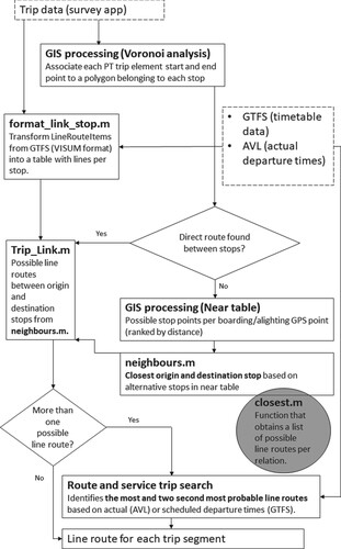
Stops were mapped onto the itineraries by usage of a geographic approach in two steps. In the first step, a stop was mapped to a boarding or alighting event if its coordinate was within a Thiessen polygon, and in the second step, neighbouring boarding/alighting stops were also taken into consideration if there was a direct PT connection with a corresponding alighting/boarding stop using the mode recorded in the survey. Finally, the line route of each PT trip leg was inferred by taking GTFS/AVL timetables and the closest possible match in time and space on line route and stop level into account (cf. Figure 1 and Berggren et al. (2019) for a detailed description of the matching procedure. A similar procedure was also successfully used by Hong et al. 2015).

Figure 1. Schematic representation of the algorithm used to infer boarding and alighting stops as well as line route(s) for each PT trip leg in the survey. GTFS – General Transit Feed Specification, AVL – Automatic Vehicle Location system.

3.3. Variables attained from survey data

For each observed trip leg in the itineraries obtained from the survey, recorded data included trip-related variables such as date, time, trip-related activities (parking, waiting or transfers exceeding two minutes in duration), mode, distance and duration. The date and time variables were used to categorise the trip into one of the seven different time periods per survey wave (year). The mode variable was used to distinguish the trip legs into PT main trip legs (all legs between the origin stop and destination stop of each trip) versus access or egress legs – the latter using one of the access/egress modes: Walk, bicycle or car. In addition, respondent characteristics such as gender and age from the survey questionnaire were appended to each observation. Trip purpose was inferred from the activity recorded by the app for each respondent before and after each trip – a record that each respondent was asked to manually validate daily.⁴ In our data, a trip was simply defined as a movement between two activities other than transfer, waiting and parking.

In the next section, the procedure of specifying and generating a set of path alternatives – choice set – for each observed trip is elaborated upon in detail.

4. Model

4.1. Choice set generation

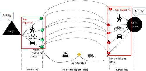
In addition to the observed trips, the data used for model estimation consisted of sets of pre-defined choice alternatives for each pair of observed activity points from the survey. All attribute data such as travel times and transfer attributes were attained from this choice set data, both for those alternatives matched with observed trips and for unused alternatives including unused transport modes. In this section, the procedure by which we generated the explicit choice set of path alternatives between activity points is outlined. A schematic outline to illustrate the structure of this procedure is presented in Figure 2. Moreover, the detailed approach to generate choice sets for the two trip leg types access/egress and PT main trips, respectively, is described in detail in Subsections 4.1.1 and 4.1.2 below.

4.1.1. Access and egress

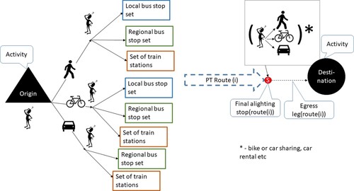
Like in the study by Marra and Corman (2020), the empirical anchor points for the generation of tentative path alternatives for the choice sets were the recorded origins and destinations of the trips in the survey (activity points in Figure 2). However, in contrast to the referred study, a tree structure of path alternatives was generated for each OD pair, where sets of unique PT stops were associated with each origin or destination point using pre-defined search criteria (Figures 2 and 3). Each criterium consisted of (1) a search range setting the maximum (shortest) network distance between the activity point and a relevant PT stop, and (2) a maximum number of relevant stops that would be considered. Thus, if more stops fell within the search range, a selection was made based on network distance. The parameters – search ranges and maximum number of considered stops – were set at unique values for each combination of access/egress mode (walk/bicycle/car) and PT mode (local bus, regional bus and train, respectively). Search ranges were set according to the distributions of observed access and egress trip legs for each access/egress and PT modal combination with the aim of including 96–98 percent of all observed access and egress trips elements.⁵ The number of alternative stops to include set with an ultimate objective to maximise the choice set overlap with observed trips. Thus, for walk access/egress trips to local bus, the 20 nearest stops within a two-kilometre (shortest path) network-wise distance from each origin/destination were selected, as were the 10 nearest train stations and major regional bus interchanges. For bicycle as access/egress mode, the criteria were set as follows: For stops serviced by local buses, the ten closest stops within five kilometres (network distance) were selected while for train stations and regional bus interchanges, ten stops satisfying these criteria were selected within a ten-kilometre network radius. Finally, for car as access/egress mode, the nearest reachable ten regional bus interchanges and train stations were searched separately within a time limit of 2.8 h along the shortest network paths (covering most of Scania). The search limits were set to ensure that the exclusion rule was not to have an adverse impact on the estimation of access and egress preferences. However, in order to limit the number of alternatives and to account for relevance in terms of availability of the access and egress modes bicycle and car for each individual, an additional restriction was applied. Travellers who did not explicitly state in the survey to have used bicycle or car for specific non home-based access or egress trips were simply assumed to not have them as tentative choice options. Thus, alternatives with car or bicycle as access (egress) mode for trips with activity at origins (destinations) other than home were removed from the choice set, if there was not a successful match for these combinations of access and egress modes with observed trips.

Figure 2. Schematic representation of the process of generating the choice set for the complete trip chain access-PT trip leg(s)-egress. Edgy shapes represent datasets while rounded shapes described process steps. Trip attributes such as travel time components were derived from the paths enumerated for the PT choice sets and access/egress choice sets, respectively, whereas personal characteristics of the travellers were retrieved from the survey through the observed trips. GTFS – General Transit Feed Specification, OSM – Open Street Map, VISUM – the software used for PT trip path generation (see also Section 4.1.2).

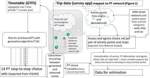
Figure 3. Choice process from trip origin to boarding stop of first PT trip leg. Route (i) represents the chosen path, where alighting stop and egress leg have a higher degree of constraint (conditionality on the chosen PT path) than the access leg. More degrees of freedom are offered when the individual has access to multiple modes at the final alighting stop, e.g. bicycle or car sharing.

All creation of stop sets per activity point was executed based on an OpenStreetMap (© OpenStreetMap contributors) layer in the ESRI ArcMap extension Network Analyst. Naturally, many of the stop sets, selected for each access and egress mode separately, overlapped, resulting in the final stop sets comprising 943 stops in the weekday 2016 timetable network and 654 stops in the 2016 weekend timetable network. For the 2017 timetable networks, the corresponding numbers were 1048 and 806 stops, respectively. These stops were defined as traffic assignment zones (centroids) in the generation of PT paths at a subsequent stage.

4.1.2. Public transport modes

In order to maximise the output of attractive paths in the choice set (Bovy 2009), and based on the theoretic discussion presented in 2.2.1 as well as findings made by Prato and Bekhor (2007) and Marra and Corman (2020), we used the branch-and-bound approach (Friedrich, Hofsaess, and Wekeck 2001) in a similar manner as Hoogendoorn-Lanser, Bovy, and van Nes (2007) to enumerate explicit PT choice sets for each time period and stop pair. The stops were selected according to the criteria for access and egress distances to activity points described in the previous subsection. Thus, separate choice sets were generated for the 14 different time periods (seven per survey wave) indicated in Table 1 in Section 3.1. The seven indicated time periods per survey wave (year) formed the basis for extracting GTFS timetables for the 2016 and 2017 survey waves, respectively, using a GTFS network that covered all regional public transport services in the region of Scania. The generation of paths was performed in the software VISUM in an all-to-all manner between the selected stops in each stop set described in the last paragraph of Section 4.1.1.

In the branch-and-bound procedure, a first general path search is performed using search impedance criteria in an unrestricted first search step (step #1). The set of alternatives hence generated is reduced in Step 2 (preselection) and subsequently forms the basis for a proportionate ranking of paths in Step 3. The ranking is made according to the value of travel disutility, or impedance, measured as perceived journey time where each trip leg type is weighed according to the design parameters in Step 3 (cf. Table 2).

Table 2. Design parameter settings/constraints applied in VISUM when performing the branch-and-bound path enumeration. FWT – waiting time at first boarding stop per trip. Coefficients, or weights, for each impedance in the search step were to be inclusive (1 for each time attribute and zero for transfer penalty) in order to minimise the restrictiveness in the path selection of the generation algorithm. S – search impedance, I – assignment impedance, JT (unweighted) total journey time, r – path, X – number of transfers.

	Weights
Step	Access	Origin wait (FWT)	In-vehicle	Egress	Transfer walk	Transfer time	Transfers (X)
1. Search	1	–	1	1	1	1	0*X
2. Preselection	$S_r\le min(S)+10$			$J{T}_r\le min(JT)+10$		$X_r\le min(X)+2,\text{J}{\text{T}}_r\le \text{min}(JT)$
3. Assignment	1	0	1	1	1	1	0

In our case, a dummy OD matrix (with an arbitrary value in each matrix element) was assigned to a PT network of each time frame in Table 1 in order to obtain sets of feasible paths per OD pair. The design parameters applied in our choice set generation framework are presented in Table 2. They were selected based on several trials, where the diversity and reasonable range of paths were key criteria. Thus, they were chosen to be as inclusive as possible, allowing for multiple alternatives for each OD (stop) pair.

In the VISUM software setup, a PT path (or combination of different line routes and, possibly, transfer stops for transfer paths) may consist of many different connections, where a connection has a unique departure time and transfer wait time. In the search step (#1), pairwise comparisons are made across all connections within each path in order to tease out one with the least search impedance, for each time period. If a connection is in no respect more feasible than another in the same time frame, then this connection is called dominated and will be discarded. This means in detail:

A connection c’ dominates a connection c, if

1. c’ lies within the time interval of c and

   1. X(c’) ≤ X(c) or

   2. SearchImp(c’) ≤ SearchImp(c)

and if real inequality applies to at least one of the three criteria or both connections are equivalent. For equivalent connections, i.e. those that only differ in transfer stops, the connection with the highest priority dominates all connections with lower priority. The priority is calculated from the sum of pre-defined walk times of the stop areas. If their priorities are the same, the connection with the earliest transfer remains available. If the stop area specific walk times of connections included in a path are equivalent, only the connection with the earliest transfer remains available.

Trip data attributes relevant to the model framework were attained from the generated PT choice sets for each time frame, with variables indicating time frame and survey year. Information regarding the number of departures per PT line, hour and stop pair were saved in order to calculate the headway of each OD path (as a proxy for waiting time at the trip origin stop).

4.1.3. Evaluation measures

In revealed preference surveys, the choice sets considered by individuals are not reported, only the chosen alternative, which makes it challenging to validate the choice sets generated (see e.g. Marra and Corman 2020). Moreover, it is not sufficient to look only at whether the observed paths are reproduced, since it is possible to continuously expand the choice sets until a high coverage is reached. The efficiency and relevance of the choice set generation approach needs also to be evaluated. Consequently, we have adopted various measures in evaluating the choice sets generated, as outlined below. Specifically, the choice set generation procedure was validated in two ways. Firstly, the generated choice set data was compared to the observations in terms of descriptive statistics. Secondly, some properties of the choice set were analysed according to an approach formulated succinctly by Rieser-Schüssler, Balmer, and Axhausen (2013). Thus, the size, reproduction rate of observed paths, path diversity and plausibility of hierarchical path sequence were evaluated. Except for the second property, i.e. the rate of reproduction of observed paths and the ability to eliminate completely unreasonable paths, there are – to the authors’ knowledge – no objective values as to when satisfactory levels of these conditions are met. However, the reproduction rate of actual observed paths may be measured in a number of ways. We applied measures of path coverage suggested by Ramming (2002) in conjunction with the measures passenger journey coverage, efficient coverage and passenger path coverage as proposed by Tan (2016) to measure this reproduction rate. The first measure, which takes into account the share of observed passengers whose observed paths are reflected in the enumerated choice set, may be calculated according to Equation (1): (1) $Co{v}_r=\frac{{\sum }_{i}I({\delta }_{r\in \{R\}})}{N_i}$(1) where the total passenger journey coverage Cov_r is conditional on the passenger (i) share of the total number of passengers N_i who have an observed path r successfully matched (included, i.e. the indicator function I(δ) = 1) to exactly one of the pre-generated choice sets {R}.

The second measure, efficient coverage Cov_e (Equation (2)), gauges the efficiency of the path enumeration by evaluating the number of generated alternatives (the size of the full path choice set {R}) required to reproduce each observed trip n (thus forming an observed and matched path r). (2) $Co{v}_e=\frac{{\sum }_{n}I({\delta }_{r\in \{R\}})}{|\{R\}|}$(2)

Finally, the third measure takes the overlap between observed and enumerated paths into account (Equation (3)). In our case, we used the link distance lv of the stop to stop PT trip part as measure of the overlap, given there was an exact match with the stop pairs of the observed and enumerated path. (3) $Co{v}_{lv}(k)=\frac{{\sum }_{n=1}^{N}I(O_{max\{r\},lv,r}\ge k)}{N}$(3) where N is the number of observations and I(·) is an indicator function equal to one whenever the overlap O of a path alternative exceeds the threshold value k. In our case, we used k value of 0.8, i.e. 80 percent of the paths in the choice set must be overlapped by an observed path, and the path with the maximum overlap for a particular OD pair was considered a match. Thus, 0.8 refers to the similarity between the observed path and the best matching path in the corresponding choice set, i.e. in the choice set a path is generated which share most of its length with the observed path. The most similar (and shortest, if there is a tie) path is assigned as the observed (if above 0.8; see also Anderson, Nielsen, and Prato 2014). We applied these three evaluating measures by calculating each of them, both for whole trips activity to activity and for PT main trip legs stop to stop, and access and egress legs separately (see Section 5.1).

4.2. Variables attained from choice set data

Each observed trip from the survey was matched to a relevant path alternative in the pre-defined choice set based on time period, stop and line identifiers as anchors between the two datasets. Thus, attributes associated with each matched trip were obtained from the choice set data. These attributes included travel times per PT mode (bus, regional train and commuter train) and access mode (walk, bicycle or car) as well as the headway of the first PT trip leg and the maximum headway per trip leg of the whole trip. The latter attributes were tested as two alternative proxies for (hidden) waiting time and adjustment time associated with the first stop of a PT trip. As noted by Frappier, Morency, and Trépanier (2018), the departure frequency of a downstream line may affect the propensity to choose a multimodal path that includes a transfer to this line. Other attributes of chosen PT path options, also obtained from the choice set, were average values of transfer-related aspects such as waiting time and walk time per transfer as well as number of transfers.

In addition, in this step a dummy variable was defined according to whether at least one boarding or transfer was made at a stop classified as being associated with an elevated level of PT passenger-relevant service.⁶

4.3. Path choice model estimation

In order to address our research questions regarding path preferences, separate model specifications were designed with respect to each of the research objectives, and each model was evaluated using multinomial logit maximum likelihood estimation. In the following subsections, these model specifications are presented. For each specification, additional covariates were added to the utility function mutually exclusively in order to enable increased model fit and to test for the influence of each covariate on utility, and thereby behaviour. Thus, we assumed utility maximisation of individual travellers and a random utility modelling framework (Ben-Akiva and Lerman 1985) when linking choice probabilities with expressed utility, the latter formulated as linear-in-parameters expression for each model specification. We included a specific path-size term (Ben-Akiva and Bierlaire 1999) in order to account for the rate of overlap across paths in the respective objective function of the model (see discussion in Section 2.2.2 for a thorough motivation).

All model estimation was performed using SAS software and the MDC procedure using multinomial logit with sampling of a maximum of 1000 alternatives for each chosen option from the full choice set using a uniform distribution.⁷

4.3.1. Basic model formulation (M1) and assumptions

A series of model specifications were tested for the systematic utility expression (V_i,n) for alternative r and individual n – the most basic one, denoted M1, is specified in Equation (4) below: (4) $\begin{array}{rl}{V}_{r,n}& ={\beta }_{t_{cw}}(t_{aw,r,i}+t_{ew,r,i})+{\beta }_{t_{cb}}(t_{ab,r,i}+t_{eb,r,i})+{\beta }_{t_{cc}}(t_{ac,r,i}+t_{ec,r,i})\\ & +{\beta }_{t_t}(t_{ro,r,i}+t_{rp,r,i})+{\beta }_{t_b}{t}_{b,r,i}+{\beta }_{t_{wkt}}{t}_{wkt,r,i}+{\beta }_{t_{tw}}{t}_{tw,r,i}+{\beta }_{fwt}FW{T}_{r,i}\\ & +{\beta }_{nTr}\text{nT}{\text{r}}_{r,i}+{\beta }_{d,cb}{\text{d}}_{cb,i}+{\beta }_{d,cc}{\text{d}}_{cc,i}+{\beta }_{lnPS}\text{ln}(P{S}_{r,i})\end{array}$(4) where t is the travel time for individual i and path r and β_t is the corresponding parameter to be estimated; cw – connection walk, aw – access walk, ew – egress walk; cb – connection bicycle, ab – access bicycle, eb – egress bicycle; cc – connection car, ac – car access, ec – car egress; t_ro – in-vehicle (ride) time regional train, t_rp – in-vehicle time commuter train, t_b – in-vehicle time bus; wkt – transfer walk; tw – transfer wait; d represents dummies for access/egress modes bicycle and car, respectively; nTr is the number of transfers per path; fwt refers to the hidden wait, or adjustment, time as derived from the minimum frequency of the chosen service measured in departures per hour ((fwt = 60/[minimum number of departures per hour]_r)/2) and PS is the path-size correction term for overlapping paths, computed as (5) $P{S}_r=\sum _{a\in {\mathrm{\Gamma }}_r}\frac{L_a}{L_r}\frac{1}{{\sum }_{s\in \{R\}}{\delta }_{a,s}}$(5) where a is a link belonging to the sets of links Γ belonging to path r, {R} is the complete choice set and δ is the link-path incidence dummy across paths r and s.

Thus, access and egress times were summed and hence assumed to affect choice preferences in a symmetric fashion. However, access and egress modes bicycle and car were assumed to be available only at the home-ends of each trips (cf. Section 4.1.1).

Assuming extreme value type 1 error terms, the probability that individual i chooses alternative r over other alternatives s is then defined as (6) $P_{r,i}=\frac{e^{V_{r,i}}}{{\sum }_{s={\{R\}}_i}^{}{e}^{V_{s,i}}},\mathrm{\forall }r,s\in \{R{\}}_i$(6) Model M1 was estimated based on both the A and the B estimation datasets, respectively, and results are henceforth referred to as stemming from the M1A and M1B models, respectively.

4.3.2. M2 – stops with elevated level of service (‘HLS stop’)

Here, a dummy variable was generated that indicated, for each path, whether there existed at least one of the stops predefined as being associated with an elevated level of passenger services such as amenities and comfort. After interacting with this dummy variable, the waiting time covariates tw (transfer wait time), nTr (number of transfers) and f (minimum departure frequency among all PT legs per trip) were once again added to the systematic utility expression of model M1 as a linear combination of parameters. Model M2 was only estimated based on the B estimation dataset, since no coefficients related to access or egress attributes were included in this model.

4.3.3. M3 – respondent characteristics

Here, the personal characteristics gender and age of each respondent, expressed as dummy variables for male and being 50 years or older, were introduced. This specific age was chosen based on the quite young ages among the survey respondents, where the median age was just 30 years old and the upper quartile 40.3 years. No respondent was older than 65 years, a common break point used when studying the preferences of PT passengers. In addition, a dummy variable for survey year 2017 was added in order to compare the time-element-specific preferences cross survey waves. To include these three dummy variables in model M5, they were interacted with all travel time and transfer-related variables in model M1 – I e t_cw, t_cb, t_cc, t_ro, t_rp, t_rb, t_wkt and t_tw. The resulting interaction variables and associated estimation parameters were subsequently included in the linear systematic utility expression. Model M3 was estimated based on both the A and the B estimation datasets, and the results are henceforth referred to as stemming from the M3A and M3B models, respectively.

4.3.4. M4 – access and egress distance

In the objective function of model M4, all access and egress travel time variables of model M1 were replaced with corresponding distance variables. The purpose was to enable the analysis of trade-offs between access and egress distance versus the other systematic components of the utility function such as travel time components other than those related to access and egress. Model M4 was only estimated based on the B estimation dataset since it focussed on coefficients of access and egress attributes.

5. Results

This section first, in Section 5.1, presents the results from the evaluation of the choice set generation procedure in terms of comparative descriptive statistics and coverage metrics, the latter as presented in Section 4.1, followed by estimation results in 5.2.

5.1. Choice set generation

In terms of general correspondence between observed trips from the survey and the generated choice set alternatives, respectively, descriptive statistics for each trip leg type were compared – see Tables 3 and 4. Particular emphasis was put on access and egress legs, since this trip leg type is usually lacking in conventional PT path choice models. Note that the exact observed paths of the access and egress legs were never matched to the choice set alternatives but only the end points (activities and first boarding/last alighting stops). As walk legs constituted about 87 percent of the observed access and egress trip legs, they have a large impact on the validity of the data. As indicated in Table 3, average walk durations are shorter among the matched observations, regardless of whether the data originate from the survey directly or from the matched choice set alternative. This may be due to longer access and egress legs potentially being more complex to match. For bicycle and car access/egress, only the choice set-matched trips have average lengths and durations shorter than in the full choice set, thus indicating an expected average preference for shorter legs among the passengers of the survey than the average choice set alternative.

Table 3. Mean access and egress attribute values, ±standard deviations, per mode for observations, observations matched to choice set and the total generated choice set. Times are in minutes and distances in metres. All choice set-derived data are taken from the ‘A’ dataset.

Attribute	Observed in survey	Observed and choice set-matched trips with data from survey	Total choice set	Choice set alternatives matched with observations – data from choice set
Access + egress walk time	14.0 ± 1.0	7.9 ± 20.3	16.6 ± 8.3	11.5 ± 6.2
Access + egress bicycle time	12.3 ± 37.4	12.3 ± 42.9	10.6 ± 10.4	8.7 ± 5.1
Access + egress car time	16.2 ± 19.0	16.3 ± 16.6	7.5 ± 4.9	6.4 ± 4.7
Access + egress walk distance	620.0 ± 4136.4	574.0 ± 822.9	1386.0 ± 689.4	955.1 ± 517.8
Access + egress bicycle distance	2128.8 ± 2673.1	2141.0 ± 2821.5	2304.1 ± 2257.9	1892.9 ± 1112.2
Access + egress car distance	8048.2 ± 12,289.2	6654.5 ± 6962.4	10,002.6 ± 13,022.0	6993.5 ± 10,198.8

Table 4. Mean main trip leg attribute values, ± standard deviations, for observations matched to choice set and the total generated choice set.

Attribute	Observed in survey	Observed and choice set-matched trips with data from survey	Total choice set	Choice set alternatives matched with observations – data from choice set
ln (Path Size) term	N/A	N/A	−0.94 ± 0.99	−0.3 ± 0.5
ln(fwt)	N/A	N/A	3.4 ± 1.5	2.3 ± 1.2
IVT bus	18.3 ± 14.3	18.0 ± 13.0	14.0 ± 10.6	15.6 ± 12.4
IVT train	37.0 ± 69.2	33.3 ± 60.0	10.4 ± 9.3	7.0 ± 16.9
Transfer walk time	6.3 ± 21.2	5.4 ± 11.7	6.5 ± 4.4	1.0 ± 2.2
Transfer wait time	8.4 ± 10.3	8.1 ± 7.0	3.0 ± 3.3	0.71 ± 2.1
Number of transfers – one	0.33 ± 0.62	0.29 ± 0.59	0.36 ± 0.48	0.18 ± 0.39
Number of transfers – many			1.3 ± 1.1	0.055 ± 0.33

Notes: Times are in minutes and distances in metres (fwt – waiting time at first trip stop). All choice set-derived data are taken from the ‘B’ dataset.

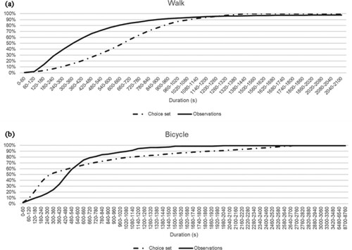
Comparative illustrations of the shorter observed walk and longer observed bicycle durations, in relation to their choice set-assumed counterparts, are found in Figure 4 by means of cumulative distributions. The values in the diagrams represent the second and the fourth column of Table 3.

Figure 4. Distribution of access and egress walk (top) and bicycle (bottom) durations, in choice set and observed trip dataset, respectively.

For the main trip part, descriptive statistics of observation-matched – ‘chosen’, – and non-chosen, alternatives are displayed in Table 4. For wait times, represented by hidden wait ahead of the trip (ln(fwt)) and transfer wait times, observation-matched choice set values were significantly shorter than those of the full choice set. However, transfer wait times measured in the survey were found significantly longer. It should be noted though that the survey values consist of events that were assigned an at least two-minute-long activity in the survey app and are thus biased upwards. For transfer walk times, the values were quite similar when the full choice set is compared to the survey data, while the chosen alternatives of the choice set were significantly shorter. The same pattern is found when comparing observed number of transfers per trip to the corresponding full choice set and matched choice set means, respectively. The very low number of transfers in the choice set data of the matched observations (rightmost column) have implications on the model estimates (cf. Section 5.2) which will be discussed in Section 6.2.

Turning to the evaluation of choice set coverage metrics, the measures passenger journey coverage, efficient coverage and passenger path coverage (Tan 2016) were used to validate our pre-defined choice and observation datasets, the results displayed in Table 5. For the first measure, 84.8 percent of the respondent passengers had at least one observed trip successfully matched to the total choice set, i.e. 15.2 percent of the survey respondents (population) were totally excluded for this particular reason from model estimation. Only 2.2 percent of the respondents had all their trips successfully matched. However, it should be noted in this context that the number of observed trips per respondent varied from one to 45 (more on data attrition in Section 6.1 below).

Table 5. Performance results from evaluation of choice set coverage based on the measures presented in Section 4.1.

Measure	Access + egress	PT trip part	Total
Passenger journey coverage (at least one trip)	91.45%	94.78%	84.76%
Passenger journey coverage (all trips)	2.60%	24.16%	2.23%
Efficient coverage	0.43%	27.59%	0.0057%
Passenger path coverage	44.88%	82.64%	39.43%

Notes: Full choice set sizes used for calculation of efficient coverage, i.e. before the sampling described in Section 4.3.

The process of data matching is outlined as a series of steps – i through to v – in Figure 7. Taken as a whole, the total passenger path coverage – for full trips – was 39 percent of the original observation set. The resulting data consist of activity-to-activity trips being matched by a full path in the choice set (1487 out of 3830 observed trips in the survey) and is henceforth denoted as the ‘A’ estimation dataset in this paper. In total, the choice set generation approach outlined in Section 4.1 and whose tree structure is illustrated in Figure 5, resulted in an activity point-to-activity point choice set of 26,255,229 distinct alternatives, i.e. 31,301.2 alternatives on average for each observed full trip that was successfully represented in the choice set (max = 332,137, median = 12,803, mode = 2, min = 1.0 and st.dev. = 40,556.5 alternatives). For the main PT part of observed trips there were 154,220 alternatives, and for access + egress 1821 alternatives generated per trip on average. The large number of alternatives for PT main trip legs compared to the choice set size of full path alternatives was caused by there being multiple stop alternatives for each activity point, as indicated in Figure 5. This entailed quite low efficient coverage figures for the full choice set, especially for access and egress legs, as indicated in Table 5 and discussed at length in Section 6.1. When evaluating one time period at a time, there were 7.99 alternatives on average stop-stop PT alternatives for the 2016 observations and 13.67 for 2017 observations, when referring to recorded trips and timetables of each survey period.

Figure 5. Schematic illustration of the choice set structure. Note that a separate set of potential initial boarding and final alighting stops were generated for each access/egress mode x PT mode combination (cf. Figure 3).

For the main PT part of trips, the total passenger path coverage was 82.6 percent. For a significant number of trips – 784 cases in total – the matching with the choice set paths failed completely (steps i-ii in Figure 7). The most common cause for mismatch between these steps, accounting for 23 percent of the mismatches, was that the mapping of the survey data to the PT network (cf. Section 3.2) failed due to a non-intuitive recorded sequence of modes in the observational data (e.g. missing PT legs). Another 19 percent were due to failure of matching of observed PT legs with a relevant PT service due to missing direct connections between recorded boarding and alighting stops. Additionally, 12 percent of the mismatches were due to the fact that the recorded PT trip itinerary was off-optimal compared to the pre-defined choice alternatives (the total travel time exceeded the pre-defined search parameters in the branch-and-bound algorithm).

For the remaining cases, the chosen threshold of 80 percent overlap between observed and pre-defined paths allowed about 95 percent of these observed trips to be covered by enumerated PT paths, as indicated in Figure 6 (and as step iii in Figure 7). A few observations with ambiguous time period affiliations in the choice set were also discarded (Step iv in Figure 7).

Figure 6. Overlap at PT path level (stop to stop) measured in share of mutual link lengths.

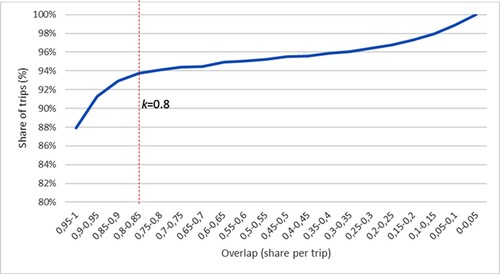
Figure 7. Illustration of data attrition in the matching process of observed trips and predefined choice sets.

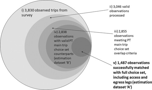
The resulting 2838 observations constitute the ‘B’ estimation dataset. The composition of individual passengers (survey respondents) in this data was somewhat different from the equivalent in the original survey dataset. In total, 18 respondents or 6.3 percent of the 268 persons participating in the survey, were lost from the original survey dataset during steps i to iv. A comparison between the survey data set and the ‘B’ estimation data set identified statistically significant differences (p < 0.05) in terms of the composition of individual characteristics as well as properties of their trips. Thus, in the estimation data set, trip distances and trip durations were shorter on average, men were more represented, and the relative frequency of work-related trip purposes was marginally higher, than in the survey sample in total. The differences in trip composition may suggest that long trips were excluded during data processing due to the fact that only regional PT trips within Scania were used as a basis for our model estimation.

A common cause of mismatches between observed and generated paths was related to missing definitions of access and/or egress trip legs – half of the observations were lost in this step (step v in Figure 7). For the access and egress legs per se, the passenger path coverage was 44.9 percent in total; for only access, it was 67.0 percent and for egress 50.2 percent. Almost half of the access/egress leg mismatches were related to non-intuitive recorded mode sequences, similarly as for the main trip mismatches. Another 13 percent could be related to trips being recorded outside of the predefined time frames in Table 1, a cause that may be referred to the design of the choice set generation framework, and an additional eight percent were related to failure to find a feasible PT service in the matching of PT legs described above.

5.2. Path choice models

All results from the parameter coefficient estimations of the models specified in Section 4.3 are presented in Table 6 for models M1 and M2 and in Table 7 for models M3 and M4, while Table 8 presents an overview of the marginal rates of substitution (MRS) for each variable in relation to the coefficient estimate for in-vehicle time (IVT) bus of that particular model, in minutes. To indicate the dataset used in each estimation, A or B is appended as a suffix to each model. Thus, M1A refers to results from model 1 based on estimation dataset A, etc. In Table 9, MRS values are presented that were calculated with bicycle access + egress distance as point of reference.

Table 6. Results from maximum likelihood estimation, based on Model M1–M2 as specified in Section 4.3.

		M1A		Model M1B		M2B
Variable type	Independent variable	Estimate	Sig.	Estimate	Sig.	Estimate	Sig.
Travel time	Access/ egress walk	−0.3506	<.0001	−0.3267	<.0001	-	-
	Access/ egress bicycle	−0.2171	<.0001	−0.2081	<.0001	-	-
	Access/ egress car	−0.4473	<.0001	−0.4253	<.0001	-	-
	IVT train	−0.0810	<.0001	−0.048	<.0001	-	-
	IVT bus	−0.0998	<.0001	−0.0777	<.0001	−0.075	<.0001
	Transfer walk	−0.1775	<.0001	−0.1072	<.0001	-	-
	Transfer wait	−0.0416	0.0319	−0.0428	0.0149	-	-
Hidden wait time		−0.3943	<.0001	−0.3070	<.0001	-	-
Number of transfers	One transfer	−4.0778	<.0001	−4.372	<.0001	-	-
	Many transfers			−8.133	<.0001
Access/egress mode dummy bicycle		−0.3626	<.0001	−0.3818	<.0001	−0.3823	<.0001
Access/egress mode dummy car		−0.5984	<.0001	−0.6314	<.0001	−0.6311	<.0001
LN PS term		1.529	<.0001	1.0242	<.0001
Stop(s) with elevated LOS	Transfer walk time	-	-	-	-	−0.1461	0.7452
	Transfer wait time	-	-	-	-	−0.0883	0.3795
	Number of transfers	-	-	-	-	−3.0227	0.013
Number of observations		1487		2838		2838
Null log-likelihood		−8318		−10,193		−10,193
Final log-likelihood		−2002		−3751		−3774
Adjusted rho-square (McFadden's LRI)		0.7593		0.632		0.6297

Notes: Estimates that are significant on 10% level are indicated in bold. Hidden wait time evaluated at median LN(FWT) = 1.90.

Table 7. Results from maximum likelihood estimation, based on Model M3–M4 as specified in Section 4.3.

		M3A		Model M3B		M4A:1
Variable type	Independent variable	Estimate	Sig.	Estimate	Sig.	Estimate	Sig.
Access/egress distance	Access/ egress distance walk	–	–	–	–	−0.0042	<.0001
	Access/ egress distance bicycle	–	–	–	–	−0.00098	<.0001
	Access/ egress distance	–	–	–	–	−0.00032	<.0001
Hidden wait time		−0.4012	<.0001	−0.3038	<.0001	−0.41252	<.0001
Number of transfers		–	–	–	–	−4.0413	<.0001
LN PS term		1.4865	<.0001	1.0806	<.0001	1.492	<.0001
Ordinary stops	Transfer walk time	–	–	–	–	−0.1939	<.0001
	Transfer wait time	–	–	–	–	−0.0524	0.0013
	Number of transfers	–	–	–	–	−4.0689	<.0001
Stop(s) with elevated LOS	Transfer walk time	–	–	–	–	−0.1042	0.4396
	Transfer wait time	–	–	–	–	−0.0390	0.8523
	Number of transfers	–	–	–	–	−3.7380	0.5715
			Number of observations (M4A:1)				1487
			Null log-likelihood (M4A:1)				−8318
			Final log-likelihood (M4A:1)				−2000
			Adjusted rho-square (McFadden's LRI, M4A:1)				0.7596
Gender = male;
Age = 50 or below (or unknown)	Access/ egress time walk	−0.3639	0.5334	–	–	M4A:2
						Estimate	Sig.
						–	–
	Access/ egress time bicycle	−0.2247	0.726	–	–	–	–
	Access/ egress time car	−0.6706	0.0052	–	–	–	–
	Access/ egress distance walk	–	–	–	–	−0.00423	0.6468
	Access/ egress distance bicycle	–	–	–	–	−0.00092	0.1317
	Access/ egress distance car	–	–	–	–	−0.00047	0.0471
	IVT train	−0.1198	0.4701	−0.0785	0.0083	−0.1259	0.0577
	IVT bus	−0.1243	0.1409	−0.0957	0.077	−0.1248	0.1154
	Transfer walk	–	–	−0.1198	0.4712	−0.2650	0.0535
	Transfer wait	–	–	−0.0169	0.0303	−0.0766	0.5802
	Number of transfers	–	–	−3.5027	0.0069	−3.2879	0.0008
Gender = male;
Age = above 50	Access/ egress time walk	−0.3201	0.5334	–	–	–	–
	Access/ egress time bicycle	−0.1644	0.7260	–	–	–	–
	Access/ egress time car	−0.3214	0.0052	–	–	–	–
	Access/ egress distance walk	–	–	–	–	−0.00395	0.6468
	Access/ egress distance bicycle	–	–	–	–	−0.00078	0.3314
	Access/ egress distance car	–	–	–	–	−0.00022	0.0471
	IVT train	−0.0099	0.1132	−0.0298	0.1248	−0.0025	0.0577
	IVT bus	−0.0459	0.2090	−0.0163	0.077	−0.0424	0.1154
	Transfer walk	–	–	−0.1565	0.669	−0.1392	0.1943
	Transfer wait	–	–	0.0203	0.2687	−0.0063	0.5802
	Number of transfers	–	–	−3.5027	0.0069	−4.5304	0.0320
Gender = female or other;
Age = 50 or below (or unknown)	Access/ egress time walk	−0.3546	<.0001	–	–	–	–
	Access/ egress time bicycle	−0.2330	<.0001	–	–	–	–
	Access/ egress time car	−0.4906	<.0001	–	–	–	–
	Access/ egress distance walk	–	–	–	–	−0.00431	<.0001
	Access/ egress distance bicycle	–	–	–	–	−0.00109	<.0001
	Access/ egress distance car	–	–	–	–	−0.00034	<.0001
	IVT train	−0.0750	0.0001	−0.024	0.0744	−0.0702	0.0006
	IVT bus	−0.1030	<.0001	−0.0733	<.0001	−0.0982	<.0001
	Transfer walk	–	–	−0.0873	0.0024	−0.1355	0.0017
	Transfer wait	–	–	−0.0936	0.0005	−0.0541	0.1417
	Number of transfers	–	–	−4.1883	<.0001	−4.4315	<.0001
Gender = female or other; Age above 50 years old	Access/ egress time walk	−0.3108	0.0353	–	–	–	–
	Access/ egress time bicycle	−0.1727	0.0457	–	–	–	–
	Access/ egress time car	−0.1414	<.0001	–	–	–	–
	Access/ egress distance walk	–	–	–	–	−0.00404	0.296
	Access/ egress distance bicycle	–	–	–	–	−0.00095	0.3314
	Access/ egress distance car	–	–	–	–	−0.0001	<.0001
	IVT train	0.0349	0.0005	0.0247	0.1248	0.0532	0.0016
	IVT bus	−0.0246	0.0002	0.0061	0.0002	−0.0158	0.0003
	Transfer walk	–	–	−0.124	0.669	−0.0097	0.1943
	Transfer wait	–	–	−0.0564	0.2687	−0.0162	0.3534
	Number of transfers	–	–	−5.7534	0.0019	−4.3612	0.032
Number of observations		1487		2838		1487
Null log-likelihood		−8318		−10,193		−8318
Final log-likelihood		−1983		−3758		−1981
Adjusted rho-square (McFadden's LRI)		0.7616		0.6313		0.7619

Note that M4 is divided in two sub-models – M4A:1 and M4A:2. Estimates that are significant at the 10% level are indicated in bold. Hidden wait time evaluated at median LN(FWT) = 1.90.

Table 8. Marginal rates of substitution (MRS – ‘weighed travel time’) in minutes, with respect to in-vehicle time bus, for trip attributes of models M1 to M3.

	All (M1)			Men 50 years or below (M3)		Men above 50 years (M3)		Women 50 years or below (M3, ref)		Women above 50 years (M3)
Parameter	A	B	HLS (M2B)	A	B	A	B	A	B	A	B
In-vehicle travel time
Bus	1.00	1.00	1.00	1.00	1.00	1.00	1.00	1.00	1.00	1.00	1.00
Train	0.81	0.62	–	0.96	0.82	0.22	1.83	0.73	0.33	−1.42	4.05
Hidden wait time	3.95	3.95	–	–	–	–	–	–	–	–	–
Access/egress time walk	3.51	4.20	–	2.93	–	6.97	–	3.44	–	12.63	–
Access/egress time bike	2.18	2.68	–	1.81	–	3.58	–	2.26	–	7.02	–
Access/egress time Car	4.48	5.47	–	5.40	–	7.00	–	4.76	–	5.75	–
Access/egress mode dummy bicycle	3.63	4.91	5.10	–	–	–	–	–	–	–	–
Access/egress mode dummy car	6.00	8.13	8.41	–	–	–	–	–	–	–	–
Transfer wait time	0.42	0.55	1.18	–	0.18	–	−1.25	–	1.28	–	*
Transfer walk time	1.78	1.38	1.95	–	1.25	–	9.60	–	1.19	–	*
Number of transfers – one	40.86	56.27	40.30	–	36.60	–	310.91	–	57.14	–	*
Number of transfers – many												104.67

Notes: Values based on coefficient estimates (Table 6) that are significant at the 10% level are indicated in bold. *Note that MRS figures for women above 50 years were not possible to derive from dataset B due to a positive sign of the coefficient for bus in-vehicle travel time estimated on that data.

Table 9. Marginal rates of substitution (MRS) from model M4, with respect to access/egress distance by bicycle (in metres), for trip attributes of model M4.

Parameter	All	HLS	Men 50 years or below	Men above 50 years	Women 50 years or below (ref)	Women above 50 years
In-vehicle travel time
Bus	100.20	–	135.95	54.50	90.17	16.65
Train	82.36	–	137.15	3.21	64.46	−56.06
Hidden wait time	396.06	–	–	–	–	–
Access/egress distance walk	4.28	–	4.60	5.08	3.96	4.25
Access/egress distance bike	1.00	1.00	1.00	1.00	1.00	1.00
Access/egress distance Car	0.32	–	0.51	0.29	0.31	0.10
Transfer wait time	54.64	39.76	83.44	8.10	49.68	−17.07
Transfer walk time	181.24	106.22	288.67	178.92	124.43	10.22
Number of transfers	4119.57	3810.40	3581.59	5823.14	4069.33	4595.57

Notes: Values based on coefficient estimates (Table 5) that are significant at a 10% level are indicated in bold.

Interestingly, all variables of model M1 contribute significantly to the estimated utility and their parameter estimates have expected signs. IVT train had a 11–38 percent lower disutility than that of travelling by bus, which is not unusual in path choice models (Anderson, Nielsen, and Prato 2014), as indicated in Table 6. As in other recent studies on PT path choice (Anderson, Nielsen, and Prato 2014; Hoogendoorn-Lanser and Bovy 2007; Tan et al. 2015), overlap of the PT part of trip paths (the Ln(PS) term) was regarded as having a positive contribution in terms of marginal utility. There was also a positive effect of departure frequency of the least frequent PT trip leg, as reflected in the negative MU of the parameter for hidden wait/adjustment time FWT. In Table 6, this coefficient is evaluated at the median FWT value (1.90 for chosen paths) due to its non-linear relationship to utility. However, there was no significant impact on path choice from departure frequency of the first PT trip leg, as indicated by additional tests (not shown in Table 6 Results from maximum likelihood estimation, based on Model M1–M2 as specified in Section 4.3. Estimates that are significant on 10% level are indicated in bold. Table 6).

In addition to the presented estimation results in Tables 6 and 7, we also tested the difference across survey years in revealed valuations of the same trip attributes, as in models M1 through to M3, in order to test robustness of estimates. For most trip attributes, we did find significant differences. However, these differences could at least partly be explained by there being differences in the observed trips across survey waves in terms of full trip duration, number of transfers per trip and in the lengths of access and egress trip legs. In general, the 2017 trips were longer and more complex than the trips of the 2016 survey (for a more exhaustive comparison of the survey waves, the reader is referred to Berggren et al. 2019).

The revealed preferences regarding access/egress time, as indicated by the MRS figures in Table 8, were quite different depending on the mode, where bicycle had the lowest measured disutility, especially compared to car. Note however the high disutility for walk as access/egress mode for women above 50 years old, a group for which car had the lowest disutility (lowest MRS figure in Table 8). The access/egress-specific dummies for bicycle and car were highly significant and highlight an extra disutility associated with these modes.

A result that stands out in particular is that there was a very high disutility associated with number of transfers (discussed in more detail in Section 6.2), especially for paths including more than one transfer (variable ‘Many transfers’); however, these were somewhat compensated by a low disutility for transfer wait time. It should be noted that there were only 77 observations with multiple transfers in a total set of 597 observed transfer trips in estimation dataset ‘B’, and, as indicated in Table 4, the mean number of transfers was very low among the observed trips/chosen alternatives of the choice set compared to the non-chosen. Moreover, when the transfer penalty variable was collapsed in specific mode combinations, we found that transfers between bus and train lines (train-bus or bus-train) contributed the most significantly to this disutility (β_{NTR,bus-train/train-bus} = −4.58, MRS(IVT_bus) = 58.74, p < 0.0001), followed by transfers across train lines (β_{NTR,train-train} = −4.20, MRS(IVT_bus) = 53.90, p < 0.0001) and bus lines (β_NTR,bus-bus = −4.11, MRS(IVT_bus) = 52.71, p < 0.0001). In this context, one should note that we were not able to retrieve transfer combinations for all trip path alternatives due to the aggregation level of the choice set. 47 percent of the path alternatives had an unknown transfer combination, which also contributed significantly to the transfer penalty (β_NTR,unknown = −3.86, p < 0.0001, MRS(IVT_bus) = 53.36).

From the MRS results of model M2B, there is a clear indication of a reduced transfer penalty for using stops with an enhanced level of service (HLS, from 56.27 to 43.24 min of IVT bus travel time, P = 0.013, for paths where there are at least one of these stops or stations used for transfer) compared to ordinary stops. Also, however less significant, walk times are valued differently (4.47 instead of 1.81 times IVT bus, P = 0.075) at HLS stops compared to ordinary ones. On the other hand, transfer wait times are not significantly different at the former stop type compared to the latter.

The respondent characteristics gender and age were used in the model formulation of M3. The coefficient for in-vehicle travel time bus for mail passengers were not rendered significant when estimations were based on dataset A. However, for female passengers, preferences indicated in Table 8 indicate a willingness to travel substantially longer by bus to avoid each access + egress minute for passengers older than 50 years, especially for walk followed by bicycle and car, compared to those 50 years and younger. For PT leg attributes, results from the B dataset indicate a systematically higher preference for paths including the train mode among younger women compared to younger men. Moreover, transfers were valued nearly ten times more tedious among men above 50 years old compared to younger men, while women of 50 years and younger valued this trip leg 36 percent less onerous than older individuals of the same gender. Unfortunately, the estimated coefficient for in-vehicle travel time bus for women above 50 years resulted in a positive sign, precluding the calculation of realistic MRS figures scaled to this value, and this was the case both for the A and B datasets. Also, the MRS value of the overlap measure – the logarithm of the path size term (ln(PS)) – is difficult to interpret in this context due to its lack of appropriate measurement unit.

Turning now to trade-offs hinging on access and egress distance made by bicycle and that may be interpreted from the MRS-values resulting from estimation results from model M4, presented in Table 9. These figures indicate the impact on the willingness to bicycle to the first or from the last stop of a trip from marginal changes in other trip attribute values. As indicated in the leftmost column of the table, passengers are on average prepared to cycle an additional 396.06 metres to reach a particular path and thus reduce the hidden wait time by one minute and 4119.57 metres extra in order to avoid a transfer. Moreover, men of age 50 or below are prepared to cycle 137.15–64.46 = 72.69 metres less than women of the same age group in order to gain one minute of train in-vehicle time, while men above 50 years old are prepared to cycle 64.46–3.21 = 61.25 metres shorter for each gained train in-vehicle minute than women at 50 years or below. Interestingly, Men and women above 50 years old are prepared to bicycle longer in order to avoid a transfer compared to younger age groups (5823.14–3581.59 = 2241.55 metres for men and 4595.57–4069.33 = 526.24 metres for women).

As for model M3, we got positive valuations for in-vehicle time train for persons above 50 years old, precluding meaningful conclusions in terms of MRS trade-offs for this group. No significant effects were found on willingness to cycle related to paths that included stops with an elevated level of service (the ‘HLS’ column of Table 9).

6. Discussion

6.1. Evaluation of choice set generation

In general, our observational data is somewhat different from the data used to estimate most PT path choice models in previous literature, in that we have detailed information regarding observed access and egress legs. This richness in observational data, however, came at a price with respect to challenges in the matching of potential paths to pre-generated choice sets when preparing data for the estimation of choice preferences, a challenge which also has been experienced in other studies that use similar choice set and revealed trip data (Marra and Corman 2020). Therefore, our accomplishments in terms of coverage may appear somewhat more modest than what has been achieved elsewhere. It should be noted, though, that a majority of the mismatches were related to imperfections of the data collection application, which resulted in trip compositions uninterpretable in the further data processing procedure. Looking at the results regarding PT main trip legs in isolation, the obtained value of the passenger path coverage metric in our study is in line with both Tan (2016) and those attained by Anderson, Nielsen, and Prato (2014) around 83 percent for an 80 percent overlap threshold.

For full door-do-door trips, Tan (2016) attained passenger path coverages of 83 percent, compared to our 39 percent of the full survey trip record, as measured between activity points. However, out of the 61 percent of non-matched observations only 17.36 percent points were referred to main PT trip mismatches. The majority of mismatches (44 percent points) could thus be attributed to errors in the matching of access or egress trip legs. Hence, as mentioned above; for both trip leg types, the most common causes for mismatch, just more than half regardless of trip leg type, were related to errors in the original data from the survey, such as unrecognisable mode sequences or off – optimal paths.

Comparing observed and pre-defined path choice sets, the differences in their respective composition (duration and length) may not have an impact on the preference estimates as long as the observed path choices are represented, and the variance is large enough in the choice set data. For access/egress walk and number of transfers, the variance of the choice set exceeded or equalled the observed variance, while the observed variance for bicycle and car access/egress legs as well as walk and wait times at transfers far exceeded their pre-defined choice set counterparts.

For the efficient coverage, the rather low outcome of just around 0.006 percent from our model setup compared to 3–5 percent in the most similar study made by Tan (2016), is largely stemming from low passenger journey coverage when all trips per respondent are considered. One important reason for this low level of passenger journey coverage is, that for each OD-pair, our methodology generates separate alternatives for each of 14 separate time frames. This framework was used in order to match each observed trip with alternatives from timetabled PT services from a relevant period. In addition, properties of the observed data, in conjunction with enumerated choice sets, has had a substantial influence on the coverage values attained. The data properties, in turn, are related to substantial levels of heterogeneity of the observed trips in terms of trip leg sequence, access and egress lengths as well as the varying conditions throughout the county of Scania, which made it necessary to relax restraints regarding maximum number of PT trip alternatives, search radii as well as number of potential access and egress stops in the generation process of the choice set. This resulted in it being quite large and an efficient coverage rate for access + egress of just 0.43 per cent. In most cases, the number of alternatives per observation is thus not equivalent to real-world conditions that actually face PT passengers (although two was actually the most common number of alternatives in the choice set). The topic of choice set composition and calibration, particularly for the definition of access and egress trip alternatives, will need future attention in discrete choice research to increase model validity.

6.2. Path choice preference values

The marginal substitution rates (MRS) we obtained, when scaling parameter estimates to in-vehicle travel time bus, are generally in line with previous studies employing smart card data for estimation of PT path choice – around 2–3 for access/egress, 0.6 for (suburban) train in-vehicle time, 0.6 for transfer wait time and 1.5 for transfer walk time (cf. corresponding figures in Anderson, Nielsen, and Prato 2014; and Tan 2016). This is despite the potentially biasing low matching rate, of observed access and egress trip legs to the corresponding pre-defined choice set alternatives, on estimated model coefficients.

However, the conspicuously high transfer penalty values, as indicated by the MRS result for number of transfers calculated from the results in model M1, deserve a further discussion. In our study, the estimated MRS for this trip attribute seems to imply that an average passenger would be willing to spend up to or more than an hour (40.86–104.67 min) of extra in-vehicle time to avoid a transfer (for model M3, the MRS is even exceeding 5 h for men older than 50). It should however be noted that there are no cases in the data set that may indicate that such a trade-off has actually been made. On the contrary, a detailed analysis of the choice sets revealed that the maximum extra in-vehicle time anyone has spent, thereby avoiding a transfer, is less than 20 min. Moreover, there are observations (although far fewer) in which passengers have indeed accepted an ‘unnecessary’ transfer, in exchange for a somewhat shorter travel time on board. We can therefore conclude that the high MRS-estimate (to intuition unrealistically high) is not supported by the limited number of cases in which real trade-off is made between travel time and transfer. Rather, the high estimate is the consequence of a steep decline of revealed choice probabilities as the number of transfers increase. This is evident in the many cases in which alternatives within the choice set offer similar qualities in other dimensions but vary in number of transfers. Longer in-vehicle times, too, have an observable, systematic and highly statistically significant impact on choice probabilities, but the relationship is not very steep. A reasonable interpretation would be that there is more variation in unmodelled attributes (larger variance of the error term) between alternatives that differ in in-vehicle time, than there is between alternatives with varying number of transfers. If this assumption is right, it would imply that a model form allowing for more flexible structure of error components might be more appropriate than the linear path size logit that we have applied to the modelling of path choice. This observation opens for interesting further research. However, it does not reduce the validity of the finding that, in our data set, an extra transfer reduces choice probabilities by almost as much as does an extra hour of in-vehicle time. As a reference, pure MRS values for transfers in relation to IVT bus is commonly estimated as being about four to six in many established state-of-the practice transport models, even though values as high as one or two hours have been found in the literature (see Iseki and Taylor 2009, for a review). A limited quantity of data in our study might have led to differences in estimated coefficients compared to results from studies where larger trip datasets have been analysed. Thus, the fact that our empirical dataset is relatively small (254 individuals and 2838 trips compared to, e.g. the Danish survey data used by Anderson, Nielsen, and Prato (2014), which comprised 2200 persons making 5641 trips), may have contributed, as could have the character of the PT network of Scania with, generally, a limited number of perceivably feasible path alternatives.

In our data, all combinations of modes seem to contribute significantly to the transfer penalty, no matter whether it was a transfer between train or bus lines. However, we found that the transfer point itself may have a significant impact on the willingness to transfer as we included the effects of en-route stations and stops with a broader-than-average range of service facilities available to passengers (‘HLS stops’) in the utility function. The impact of station and interchange design is analysed and discussed further by Eltved (2020), who found that facilities such as shops and relative ease of wayfinding significantly lower the transfer penalty. In addition, there might have occurred a similar phenomenon in our PT path choice results as that found among motorists when landmark points are used for navigating in the road geography, as reported by inter alia Ramming (2002), but, for PT stops, the utility of using HLS stops could be more explicitly related to en-route errands or the like. A factor that may have contributed to the high disutility associated with transfers is the quite simple regional PT network structure in Scania compared to large metropolitan regions. In the Scania network, there are very few opportunities to change and thus arrive earlier than when sticking to the same connection without transferring. As we have observed elsewhere (Berggren et al. 2019), there seem to be latent factors, particularly affecting the 2017 survey observations, that influenced path choice and thus decreased the revealed preference values for direct trips.

To our knowledge, some of the variables of our access and egress mode framework have not previously been tested for their potential impact on path preferences. Here we found, as is indicated by the MRS values for the mode-specific dummies, that both bicycle and car entail extra disutility that is not captured in the travel times of these modes. This extra disutility may be related to omitted travel time attributes in the choice set such as parking and moving from the private vehicle to the PT stop or station. In line with the findings of Ton et al. (2020), we found reasonable trade-off values for path attributes such as hidden wait time, for stops with elevated levels of service (perhaps corresponding to bus/tram hubs used by Ton et al. 2020) when measured in bicycle access + egress distance. Similar to their results, we get higher willingness to cycle to gain in-vehicle travel time among younger age groups (50 years or younger) compared to travellers older than 50 years – at least for female travellers for bus trips, and an even more pronounced such tendency in relation to in-vehicle travel time train for male passengers.

There appears to be a discrepancy in the underlying behavioural or perceptual mechanisms between the correlation patterns of road and public transport paths, specifically when evaluating the sign and values of the path size term in path size logit (Askegren Anderson 2013; Hoogendoorn-Lanser and Bovy 2007). Hoogendoorn-Lanser and Bovy (2007) found, when evaluating different path size formulations on a multimodal network based on intercity rail as the main mode, that using different path size terms for sub-paths from different parts of the trips, the effect of the overlaps varied – from a positive effect on the main mode (trip legs using rail) to negative effects on access and egress legs. Moreover, Tan et al. (2015) successfully applied a frequency-based path size term in addition to the distance-based path size term when estimating path choice models in a multimodal network. These pieces of evidence may suggest that individuals with complete freedom in their routeing behaviour (e.g. car drivers) tend to prefer paths with few minimally diverging auxiliary path alternatives, like main arterial roads, while PT passengers prefer corridors with multiple services and thus a high relative departure frequency (Hoogendoorn-Lanser and Bovy 2007).

7. Conclusion

Smartphone app survey-based empirical trip data was utilised in the analysis outlined in this paper in order to form the basis of an approach to find revealed path choice preferences for PT trips in Scania County, south Sweden. Using detailed explicit path sets, including connecting access and egress trip legs between activities and first and last stops of the PT trip part, enabled us to explore PT path choice in an unusually detailed fashion. An important aspect in this exploration was the desire to relate the outcome from this fairly recent form of data collection to more established approaches in terms of both the efficiency of the method and the validity of the resulting preference values. It is fair to say that our approach, being in its infancy, has some more to prove in terms of output rate and coverage with pre-defined paths – at least for access and egress legs. However, we found that most of data loss could be referred to imperfections in collected trip data related to properties of the survey instrument. The data processing and estimation framework themselves seem to work quite well in terms of the fact that reasonably few observations were lost during these procedural instances. Continuous improvement of survey technology based on smartphones will likely improve the quality of recorded trip information over time. There may be method-specific factors that have significant impact on the estimates presented here, e.g. those for transfers, in comparison to estimates that underlie state-of-the practice models – the latter usually based on revealed data from pen-and-paper or telephone-based single day travel surveys or stated choice data. Future studies should focus on comparing and benchmarking these preference values in a systematic manner across data collection approaches.

We believe that the main contribution of this paper lies in the utilisation of a reasonable novel source of detailed revealed behavioural data that go beyond established methods regarding the combined detailedness and comprehensiveness (door-do-door) properties of the data. Moreover, we corroborate this strength by showing that we were able to obtain PT passengers’ preference values comparable to those regarded as valid in the research community of the field. In addition, we were able to expand on the range of possible preference attributes typically estimated, facilitated by the comprehensiveness and detailedness of the empirical data source of trip data.

There are a number of intriguing new avenues for future research making further use of this kind of detailed longitudinal travel data. Particularly interesting could be to explore the possible systematic correlation in revealed preferences in different choice situations for each individual in contrast to systematic differences between individuals. Making full use of the longitudinal properties of the survey data, in order to study dynamic day-to-day or weekly variation in preferences, is also left for further research endeavours. Moreover, including travel time uncertainty in the utility specification would enable a closer study of the passenger routeing effects from small but common delays and service disruptions.

Acknowledgements

The authors wish to express their warm gratitude to these organisations. In addition, we are most grateful to the public transport provider in the region of Scania (Skånetrafiken) for their kind contribution of real-time vehicle location data. The authors also wish to thank the four anonymous reviewers for their valuable contributions in improving this paper. This research was performed in collaboration with K2 – The Swedish Knowledge Centre for Public Transport.

Disclosure statement

No potential conflict of interest was reported by the author(s).

Data availability

The personal mobility data forming the basis of this paper does not reveal sensitive personal information. However, the data cannot be made publicly available due to their disaggregate form that makes it possible to follow individuals’ movements. All data that support the findings of this study may be available on request from the corresponding author, U. Berggren.

Additional information

Funding

The research presented in this paper was made possible thanks to two sources of funding: Trafikverket/Swedish Transport Administration [grant number TRV 2016/10730] and the EU Interreg programme Öresund-Kattegat-Skagerrak, specifically the EU project: [NYPS 202015553].

Notes

1 At user equilibrium in a flow-dependent network, no single traveller can reduce her travel time by unilaterally changing path, and this implies that the travel time are equal across all used paths at user equilibrium.

2 The decision to use two waves was based on the ambition to obtain a panel sample based on repeated observations for the same individuals during the two years (survey waves). However, as less than five percent of the participants of the first wave recurred during the second wave, this approach had to be abandoned.

3 General Transit Format Specification – data format for public transport lines, line routes, time profiles and vehicle journeys originally specified by Google. The Swedish database provided by Samtrafiken AB via https://www.trafiklab.se.

4 In the validation phase, the respondent was offered a set of available options, and after being entered once at a particular location, the app suggested the same activity option the next time (s)he arrived at the same location with her/his phone.

5 The exact choice of percentage limits was set according to the empirical distribution of distances in the access and egress legs of the survey in order to exclude obvious outliers and to be reasonably in line with maximum access and egress distances found in the literature.

6 This included amenities such as shops, restaurants and cafés, and the stops denoted with this flag consisted of major train stations and bus interchanges.

7 The sample size of the choice set was chosen somewhat arbitrarily. However, in doing so, we considered the combinatorial potential of including 10*10 access-egress combinations per mode and adding the mean number of PT main trip paths of 37, as reported by Anderson, Nielsen, and Prato (2014). When comparing parameter estimate values, going from 30,000 (containing the mean choice set size per activity pair) to 1000 sampled path options did not change these values significantly.

References

- Alizadeh, H., B. Farooq, C. Morency, and N. Saunier. 2019. “Frequent Versus Occasional Drivers: A Hybrid Route Choice Model.” Transportation Research Part F: Traffic Psychology and Behaviour 64: 171–183. doi:10.1016/j.trf.2019.05.009.
- Allström, A., G. Gidofalvi, I. Kristoffersson, A. C. Prelipcean, C. Rydergren, Y. Susilo, and J. Widell. 2016. Experiences from Smartphone Based Travel Data Collection – System Development and Evaluation. Stockholm.
- Anderson, M. K., O. A. Nielsen, and C. G. Prato. 2014. “Multimodal Route Choice Models of Public Transport Passengers in the Greater Copenhagen Area.” EURO Journal on Transportation and Logistics 6 (3): 221–245. doi:10.1007/s13676-014-0063-3.
- Askegren Anderson, M. K. 2013. “Behavioural Models for Route Choice of Passengers in Public Transport.” PhD Doctoral disertation. DTU, Copenhagen, Denmark.
- Bagherian, M., O. Cats, N. van Oort, and M. Hickman. 2016. “Measuring Passenger Travel Time Reliability using Smart Card Data.” Paper presented at the TRISTAN IX: Triennial Symposium on Transportation Analysis, Oranjestad, Aruba.
- Ben-Akiva, M., M. Bergman, A. J. Daly, and R. Ramaswamy. 1984. “Modeling Inter-Urban Route Choice Behaviour.” Proceedings of the 9th International Symposium on Transportation and Traffic Theory, VNU Press, Utrecht, 299–330.
- Ben-Akiva, M., and M. Bierlaire. 1999. “Discrete Choice Methods and Their Applications to Short Term Travel Decisions.” In Handbook of Transportation Science, edited by R. W. Hall, 5–33. Boston, MA: Springer US.
- Ben-Akiva, M., and S. R. Lerman. 1985. Discrete Choice Analysis - Theory and Application to Travel Demand. Cambridge, Massachusetts: MIT Press.
- Berggren, U., C. Johnsson, H. Svensson, and A. Wretstrand. 2019. “Exploring Waiting Times in Public Transport Through a Semi-Automated Dedicated Smartphone app Survey.” Travel Behaviour and Society 15: 1–14. doi:10.1016/j.tbs.2018.11.002.
- Bovy, P. H. L. 2009. “On Modelling Route Choice Sets in Transportation Networks: A Synthesis.” Transport Reviews 29 (1): 43–68. doi:10.1080/01441640802078673.
- Chang, Y.-J., G. Paruthi, H.-Y. Wu, H.-Y. Lin, and M. W. Newman. 2017. “An Investigation of Using Mobile and Situated Crowd Sourcing to Collect Annotated Travel Activity Data in Real-Word Settings.” International Journal of Human-Computer Studies 102: 81–102. http://doi.org/10.1016/j.ijhcs.2016.11.001.
- Clark, A., E. Adell, A. Nilsson, and L. Indebetou. 2017. Detaljerad kartläggning av verktyg och applikationer för resvaneundersökningar.
- Cottrill, C. D., F. C. Pereira, F. Zhao, I. F. Dias, H. B. Lim, M. E. Ben-Akiva, and P. C. Zegras. 2013. “Future Mobility Survey.” Transportation Research Record: Journal of the Transportation Research Board 2354 (1): 59–67. doi:10.3141/2354-07.
- Danaf, M., B. Atasoy, C. L. de Azevedo, J. Ding-Mastera, M. Abou-Zeid, N. Cox, F. Zhao, and M. Ben-Akiva. 2019. “Context-Aware Stated Preferences with Smartphone-Based Travel Surveys.” Journal of Choice Modelling 31: 35–50. doi:10.1016/j.jocm.2019.03.001.
- de la Barra, T., B. Perez, and J. Anez. 1993. “Multidimensional Path Search and Assignment.” Proceedings of PTRC Summer Annual Meeting, 21st, 1993, University of Manchester, United Kingdom.
- Dyrberg, M. B., C. B. Christensen, M. K. Anderson, O. A. Nielsen, and C. G. Prato. 2015. “Transfer Attributes in Route Choice Models for Public Transport Passengers.” Paper presented at the hEART.
- Eltved, M. 2020. “Modelling Passenger Behaviour in Mixed Scheduleand Frequency-Based Public Transport Systems.” PhD disertation. Danmarks Tekniske Universitet, Copenhagen.
- Fiorenzo-Catalano, S., R. van Nes, and P. H. L. Bovy. 2004. “Choice Set Generation for Multi-Modal Travel Analysis.” EJTIR 4 (2): 195–209.
- Florida, R. 2018. The new Urban Crisis Paperback ed. New York: Basic Books.
- Fonzone, A., J.-D. Schmöcker, M. Bell, G. H. Gentile, F. Kurauchi, K. Nökel, and N. H. M. Wilson. 2010. “Do Hyper-Travellers Exist? Initial Results of an International Survey on Public Transport User Behaviour.” Paper presented at the 12th WCTR, Lisbon, Portugal.
- Frappier, A., C. Morency, and M. Trépanier. 2018. “Measuring the Quality and Diversity of Transit Alternatives.” Transport Policy 61: 51–59. doi:10.1016/j.tranpol.2017.10.007.
- Friedrich, M., I. Hofsaess, and S. Wekeck. 2001. “Timetable-Based Transit Assignment Using Branch and Bound Techniques.” Transportation Research Record 1752 (1): 100–107. doi:10.3141/1752-14.
- Gadziński, J.. 2018. “Perspectives of the Use of Smartphones in Travel Behaviour Studies: Findings from a Literature Review and a Pilot Study.” Transportation Research Part C: Emerging Technologies 88: 74–86. http://doi.org/10.1016/j.trc.2018.01.011.
- Garcia-Martinez, A., R. Cascajo, S. R. Jara-Diaz, S. Chowdhury, and A. Monzon. 2018. “Transfer Penalties in Multimodal Public Transport Networks.” Transportation Research Part A: Policy and Practice 114: 52–66. doi:10.1016/j.tra.2018.01.016.
- Gentile, G., M. Florian, Y. Hamdouch, O. Cats, and A. Nuzzolo. 2016. “The Theory of Transit Assignment: Basic Modelling Frameworks.” In Modelling Public Transport Passenger Flows in the Era of Intelligent Transport Systems: COST Action TU1004 (TransITS), edited by G. Gentile and K. Noekel, 287–386. Cham: Springer International Publishing.
- Geurs, K. T., T. Thomas, M. Bijlsma, and S. Douhou. 2015. “Automatic Trip and Mode Detection with Move Smarter: First Results from the Dutch Mobile Mobility Panel.” Transportation Research Procedia 11: 247–262. http://doi.org/10.1016/j.trpro.2015.12.022.
- Hong, S.-P., Y.-H. Min, M.-J. Park, K. M. Kim, and S. M. Oh. 2015. “Precise Estimation of Connections of Metro Passengers from Smart Card Data.” Transportation 43 (5): 749–769. doi:10.1007/s11116-015-9617-y.
- Hoogendoorn-Lanser, S., and P. Bovy. 2007. “Modeling Overlap in Multimodal Route Choice by Including Trip Part-Specific Path Size Factors.” Transportation Research Record: Journal of the Transportation Research Board 2003 (1): 74–83. doi:10.3141/2003-10.
- Hoogendoorn-Lanser, S., P. Bovy, and R. van Nes. 2007. “Application of Constrained Enumeration Approach to Multimodal Choice Set Generation.” Transportation Research Record: Journal of the Transportation Research Board 2014 (1): 50–57. doi:10.3141/2014-07.
- Ingvardson, J. B., O. A. Nielsen, S. Raveau, and B. F. Nielsen. 2018. “Passenger Arrival and Waiting Time Distributions Dependent on Train Service Frequency and Station Characteristics: A Smart Card Data Analysis.” Transportation Research Part C: Emerging Technologies 90: 292–306. doi:10.1016/j.trc.2018.03.006.
- Iseki, H., and B. D. Taylor. 2009. “Not All Transfers Are Created Equal: Towards a Framework Relating Transfer Connectivity to Travel Behaviour.” Transport Reviews 29 (6): 777–800. doi:10.1080/01441640902811304.
- Lee, R. J., I. N. Sener, and J. A. Mullins. 2016. “An Evaluation of Emerging Data Collection Technologies for Travel Demand Modeling: From Research to Practice.” Transportation Letters 8 (4): 181–193. http://doi.org/10.1080/19427867.2015.1106787.
- Marra, A. D., and F. Corman. 2020. “Determining an Efficient and Precise Choice set for Public Transport Based on Tracking Data.” Transportation Research Part A: Policy and Practice 142: 168–186. doi:10.1016/j.tra.2020.10.013.
- McFadden, D., and K. Train. 2000. “Mixed MNL Models for Discrete ResponsE.” Journal of Applied Econometrics 15: 447–470.
- Nassir, N., M. Hickman, and Z.-L. Ma. 2015. “Behavioural Findings from Observed Transit Route Choice Strategies in the Farecard Data of Brisbane.” Paper presented at the Australasian Transport Research Forum 2015, Sydney, Australia. https://www.atrf.info/papers/index.aspx.
- Nielsen, O. A. 2000. “A Stochastic Transit Assignment Model Considering Differences in Passengers Utility Functions.” Transportation Research Part B: Methodological 34: 377–402.
- Prato, C. G. 2009. “Route Choice Modeling: Past, Present and Future Research Directions.” Journal of Choice Modelling 2 (1): 65–100. doi:10.1016/s1755-5345(13)70005-8.
- Prato, C. G., and S. Bekhor. 2007. “Modeling Route Choice Behavior.” Transportation Research Record: Journal of the Transportation Research Board 2003 (1): 64–73. doi:10.3141/2003-09.
- Prelipcean, A. C., G. Gidófalvi, and Y. O. Susilo. 2018. “MEILI: A Travel Diary Collection, Annotation and Automation System.” Computers, Environment and Urban Systems 70: 24–34. http://doi.org/10.1016/j.compenvurbsys.2018.01.011.
- Ramming, S. M. 2002. “Network Knowledge and Route Choice.”
- Raveau, S., J. C. Muñoz, and L. de Grange. 2011. “A Topological Route Choice Model for Metro.” Transportation Research Part A: Policy and Practice 45 (2): 138–147. doi:10.1016/j.tra.2010.12.004.
- Rieser-Schüssler, N., M. Balmer, and K. W. Axhausen. 2013. “Route Choice Sets for Very High-Resolution Data.” Transportmetrica A: Transport Science 9 (9): 825–845. doi:10.1080/18128602.2012.671383.
- Seaborn, C., J. Attanucci, and N. H. M. Wilson. 2009. “Analyzing Multimodal Public Transport Journeys in London with Smart Card Fare Payment Data.” Transportation Research Record: Journal of the Transportation Research Board 2121 (1): 55–62. doi:10.3141/2121-06.
- Sheffi, Y. 1985. Urban Transportation Networks: Equilibrium Analysis with Mathematical Programming Methods. Englewood Cliffs, New Jersey: Prentice Hall.
- Stopher, P. R., and S. P. Greaves. 2007. “Household Travel Surveys: Where are we Going?” Transportation Research Part A: Policy and Practice 41 (5): 367–381. doi:10.1016/j.tra.2006.09.005.
- Stopher, P. R., L. Shen, W. Liu, and A. Ahmed. 2015. “The Challenge of Obtaining Ground Truth for GPS Processing.” Transportation Research Procedia 11: 206–217. http://doi.org/10.1016/j.trpro.2015.12.018.
- Tan, R. 2016. “Modeling Route Choice Behaviour in Public Transport Network.”
- Tan, R., M. Adnan, D.-H. Lee, and M. E. Ben-Akiva. 2015. “New Path Size Formulation in Path Size Logit for Route Choice Modeling in Public Transport Networks.” Transportation Research Record: Journal of the Transportation Research Board 2538 (1): 11–18. doi:10.3141/2538-02.
- Ton, D., S. Shelat, S. Nijënstein, L. Rijsman, N. van Oort, and S. Hoogendoorn. 2020. “Understanding the Role of Cycling to Urban Transit Stations Through a Simultaneous Access Mode and Station Choice Model.” Transportation Research Record: Journal of the Transportation Research Board 2674 (8): 823–835. doi:10.1177/0361198120925076.
- van der Zijpp, N. J., and S. Fiorenzo Catalano. 2005. “Path Enumeration by Finding the Constrained K-Shortest Paths.” Transportation Research Part B: Methodological 39 (6): 545–563. doi:10.1016/j.trb.2004.07.004.
- Wang, Z., S. Y. He, and Y. Leung. 2018. “Applying Mobile Phone Data to Travel Behaviour Research: A Literature Review.” Travel Behaviour and Society 11: 141–155. http://doi.org/10.1016/j.tbs.2017.02.005.
- Zhao, F., F. C. Pereira, R. Ball, Y. Kim, Y. Han, C. Zegras, and M. Ben-Akiva. 2019. “Exploratory Analysis of a Smartphone-Based Travel Survey in Singapore.” Transportation Research Record: Journal of the Transportation Research Board 2494 (1): 45–56. doi:10.3141/2494-06.
- Zhao, J., and A. Rahbee. 2007. “Estimating a Rail Passenger Trip Origin-Destination Matrix Using Automatic Data Collection Systems.” Computer-Aided CIvil and Infrastructure Engineering 22: 376–387.