Joint optimisation of regular and demand-responsive transit services

ABSTRACT

This study aims to jointly optimise regular and demand responsive transit (DRT) services, which can offer opportunities for leveraging on their respective advantages. An optimisation model with the objective of minimising the total travel time of passengers and the total fleet size is proposed. The terminal bus stops of regular bus lines, the service area of the DRT, and the fleet size of both regular and DRT are optimised simultaneously. A rule-based optimisation preparation step is added to the proposed model to obtain a reasonable design scheme and to reduce the computational load. The model is solved using a tailored boundary-start-based two-step heuristic algorithm. The performance of the mixed network is affected by the preference of the decision maker and the operation mode adopted for the DRT service. A reduction in the operational level of the DRT results in a considerable increase in the travel time of DRT passengers.

KEYWORDS:

• Transit network design
• joint optimisation
• demand responsive transit
• bus systems

1. Introduction

Transit is regarded as one of the backbones of sustainable urban development (SuM4All 2017). Giving priority to the development of transit is a strategic choice to alleviate traffic congestion, transform urban traffic development mode, and contribute to an environment-friendly society. The concept of Mobility-as-a-Service (MaaS) has emerged in the field of transportation with the booming development of the sharing economy in recent years. Moreover, Demand Responsive Transit (DRT) – delivered in various forms ranging from flexible feeder services to ride-hailing – increasingly offers a personalised travel service and can dynamically match supply and demand (Calderón and Miller 2020; Alonso-González et al. 2020).

The different transit service modes have distinctive characteristics. Regular line-based transit has a large carrying capacity, while the DRT with flexible operation scheduling might be more suitable in the case of low demand density. Therefore, how to integrate various services while leveraging on their respective advantages becomes a crucial challenge in improving the level-of-service offered by joint transit services. This study aims to jointly optimise the regular line-based and schedule-based service with DRT services, including determining lines, stops, and fleet sizes, on the basis of the existing transit network.

The transit network design (TND) problem has been addressed by researchers in the last decades (Lampkin and Saalmans 1967; Holroyd 1967; Byrne and Vuchic 1972; Kepaptsoglou and Karlaftis 2009). A significant volume of works has been conducted. The following paragraphs offer a brief review of the research developments on the transit network design in three regards: the regular transit service, the DRT service, and the joint planning.

For the regular transit service, the transit network planning problem is typically divided into strategic, tactical, and operational levels (Desaulniers and Hickman 2007; Ceder 2007; Ibarra-Rojas et al. 2015; Zhao et al. 2019; Gkiotsalitis 2021). At the strategic level, the bus lines and stops are designed according to the topology conditions and the origin-destination (OD) demands. The modelling methods of the TND problem can be divided into two categories: the discrete optimisation approach and the continuous approximations approach (Guihaire and Hao 2008; Ibarra-Rojas et al. 2015). At the tactical level, the service frequency, fleet size, and departure and arrival times of buses are determined according to the transit routes network and OD demand patterns. The rule-based approaches were used in early works based on the fixed demand-line assignment assumption. Then, the bi-level approaches were proposed to optimise the frequency and demand for bus lines with the consideration of the transit assignment (Desaulniers and Hickman 2007; Guihaire and Hao 2008; Ibarra-Rojas et al. 2015). To better cater for passenger demand, several works have jointly addressed the abovementioned strategic and tactical problems for the regular transit service, implying that the route design and the frequency setting are optimised in a unified framework. The bus route network and schedules were first jointly designed (Yan and Chen 2002; Zhao and Zeng 2008; Szeto and Wu 2011; Arbex and da Cunha 2015). Some other studies further integrated the consideration of the transit operational mode, such as short-turning and interlining lines, into the transit network design and frequency setting problem (Gkiotsalitis, Wu, and Cats 2019; Oliker and Bekhor 2020). With the increase of the complexity of the integrated model, the rule-based scheme methods were proposed in these two studies to obtain a realistic design.

For the DRT, the planning and design at the strategic and tactical levels have attracted extensive attention in recent years. The pricing strategy, service area, fleet size, departure frequency, dispatching strategy, and service routes of the DRT service have been investigated. To be attractive to customers, the service area and the forward progression velocity (velocity along the direction) were first considered (Quadrifoglio, Hall, and Dessouky 2006). Diana, Quadrifoglio, and Pronello (2007) discussed the least polluting transit system based on the emission model, in which the travelled distance between a traditional fixed-route and a demand responsive transit service were compared. Daganzo and Ouyang (2019) presented a general analytic framework to model the door-to-door transit service, including non-shared taxi, dial-a-ride, and ridesharing. The dispatching strategy and fleet size were discussed. Kim, Levy, and Schonfeld (2019) optimised the headway and service zone size of the flexible-route bus system with the objective of minimising the average cost per passenger trip. Huang et al. (2020) optimised the route of DRT with the objective of maximising the benefits of the system while considering the preferred time windows of passengers. Wang et al. (2020) proposed a two-step coordinated optimisation model, in which the vehicle running route and schedule and the response to the passenger’s real-time application were optimised, respectively. Franco, Johnston, and McCormick (2020) developed an agent-based model to predict the performance of a DRT service using an activity-based approach. Mehran, Yang, and Mishra (2020) proposed a semi-flexible transit service that runs along a fixed route, a limited number of fixed stops, and a flexible schedule. Zhang et al. (2021) optimised the routing problem of the suburban DRT service, in which the number of rental vehicles and routing were decided simultaneously. Li et al. (2021) proposed a demand-responsive connector bus operational network with the consideration of passengers’ predefined service time windows. Wang et al. (2021) established an optimisation of running route and scheduling for responsive feeder transit under mixed demand of the time-dependent road network. The travel time variability is considered in these models. However, these studies optimised the DRT service without the consideration of the regular transit.

The co-existence of regular transit and DRT pushes researchers to revisit the design of public transit systems and in particular examine efficient ways to combine the two types of transit services. The simulation-based model and empirical-based model are two mainly applied method. Mendes, Bennàssar, and Chow (2017) established an event-based simulation model to compare the performance of the shared autonomous vehicle system with the light rail system in New York City. Scheltes and de Almeida Correia (2017) proposed an agent-based simulation model to analyse the performance of the automated last-mile transport system. Winter et al. (2018) analysed the effects of demand levels, vehicle capacity, vehicle dwell time, and the initial vehicle distribution on system performance. Basu et al. (2018) proposed a multi-modal agent-based urban simulation platform to investigate the effects of the automated mobility-on-demand service on urban transportation. Shen, Zhang, and Zhao (2018) proposed an operational scenario for integrating shared autonomous vehicles into the regular transit system to improve the first-mile service during morning peak hours. Coutinho et al. (2020) conducted a before and after comparison based on the empirical case in Amsterdam, the Netherlands. The regular bus service in low-density areas was replaced by a DRT one, resulting in a better overall efficiency. These studies either replace specific transit routes with DRT or add the DRT to the existing regular transit network. Few studies have considered the real joint planning of regular transit and DRT. Pinto et al. (2020) proposed a joint design method for the regular transit and shared-use autonomous vehicles services (SAMS). The frequencies of the regular transit and the fleet size of SAMS were optimised.

It can be thus concluded that although much is known about the design of regular transit and DRT, they are usually modelled as two separate systems, hence disregarding the interactions between these two services. These designs have insofar predetermined that a trip or a region is to be served by one type of service.

In this study, we formulate and solve the joint optimisation of regular transit and DRT networks. In the optimisation, the passengers are allowed to use any one or combination of the two transit services. For regular transit network, the terminal (start/end) bus stops and the fleet size of each bus line are optimised. For DRT network, the service area and the fleet size are optimised. Our model aims to reduce the total travel time for passengers as well as the total fleet size for transit agencies. Therefore, a mutually beneficial transit planning can be obtained. The contribution of this study lies in that the bus lines and fleet size of the regular transit and DRT are simultaneously optimised in a unified framework allowing for the consideration of trade-offs between the two services.

The remainder of the paper is organised as follows. Section 2 describes the joint optimisation problem and model for regular and DRT networks. The tailored solution algorithm is presented in Section 3. In Section 4 we analyse the performance of the model with a case study and sensitivity analysis. Conclusions and a discussion of future research directions are given in Section 5.

2. Joint service design optimisation model

The joint optimisation problem and model for regular and DRT networks are established in this section. The joint service representation and the framework of the optimisation model are first introduced. Then the detailed description of each part of the model is presented.

2.1. Joint service representation

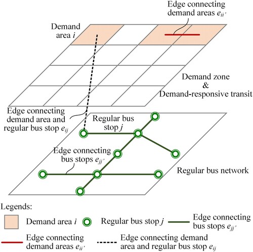
Before presenting the formulation, we first clarify the terms related to the adjustment of the regular transit lines and the setting of the DRT line. The topological graph of the joint service is illustrated in Figure 1. In the context of this work, the original regular transit line can be shortened. The adjusted regular transit line serves all stops of a segment of the original regular transit line in both directions. However, the regular transit line can neither be extended nor a new line can be added. For the setting of the DRT line, all the neighbouring demand areas in the DRT network are served with the DRT service. The DRT line should at least consist of two neighbouring demand areas.

Figure 1. Topological graph of the joint service.

The core of the optimisation is a non-linear programming model (Section 2.4) to minimise the total travel time of passengers and the total fleet size. To obtain a reasonable design scheme and to reduce the computational load, a preparation step (Section 2.3) is added at the beginning of the optimisation process.

2.2. Notations

To facilitate model presentation, notations used hereafter are summarised in Table 1. They are divided into three categories: input variables, decision variables, and auxiliary variables. The inputs of the optimisation model include the network topology, the initial fleet size of regular bus lines, travel time, and passenger OD demand. The proposed model aims to optimise the terminal (start/end) bus stops of regular bus lines ($g_l^s$ and $g_l^e$), the service area of the DRT (${\beta }_i$), and the fleet size of both regular and DRT ($m_l^B$ and $m^R$) are optimised in a unified framework.

Table 1. Notation of key model parameters and variables.

Input variables
$I$	Set of demand areas
$i\in I$	Index of demand areas
$J$	Set of regular bus stops
$j\in J$	Index of regular bus stops
$L$	Set of regular bus lines
$l\in L$	Index of regular bus lines
$B$	Superscript $B$ indicates that the parameter is related with regular transit
$R$	Superscript $R$ indicates that the parameter is related with DRT
$n_l^B$	Initial fleet size of regular bus line $l$, vehicles
$N$	Fleet size limits, vehicles
$p_l$	Number of bus stops of bus line $l$
$J_l$	Set denoting the bus stops of line $l$ in a sequential order
$t_{j{j}^{\mathrm{\prime }}}^B$	Travel time of regular transit from bus stop $j$ to bus stop $j{}^{\mathrm{\prime }}$, h
$t_{ij}^C$	Travel time between demand area $i$ and bus stop $j$, h
$t_{i{i}^{\mathrm{\prime }}}^R$	Travel time of DRT between demand areas $i$ and $i{}^{\mathrm{\prime }}$, h
$t_r$	Penalty time for the transferring, h
$d_{i{i}^{\mathrm{\prime }}}$	Passenger demand from demand area $i$ to demand area $i{}^{\mathrm{\prime }}$, person/h
$K^B$, $K^R$	Vehicle capacity for regular transit and DRT, person
$\alpha$	Weight factor that convert the fleet size into units of time
${\gamma }_t$	Penalty factor for the waiting time against the in-vehicle time
${\gamma }_w$	Waiting time coefficient of the DRT
${\gamma }_c$	Fleet size coefficient of DRT
$\delta$	Threshold value of ridership upon which a bus stop can be considered to be removed, person/h
$\tau$	Threshold value of travel time between demand area and bus stop upon which a demand area can be considered to be served by the DRT, h
$\epsilon$	Threshold value of the stopping criteria in GA
Decision variables
$g_l^s$, $g_l^e$	Adjusted start and end bus stops of regular bus line $l$
${\beta }_i$	Binary variable for the demand area $i$ served by the DRT, 1 – yes, 0 – no
$m_l^B$	Adjusted fleet size of regular bus line $l$, vehicles
$m^R$	Fleet size of DRT, vehicles
Auxiliary variables
$Z$	Set of DRT routes
$z\in Z$	Index of possible DRT routes
$T$	Total travel time of passengers, h
$C$	Total fleet size of transit lines, vehicles
$S_l^s$, $S_l^e$	Set of potential adjusted start and end bus stops of bus line $l$
$S_r$	Set of potential removed bus stops
$S_d$	Set of potential demand areas served by the DRT
$T_{i{i}^{\mathrm{\prime }}}$	Travel time of passengers from demand area $i$ to demand area $i{}^{\mathrm{\prime }}$, h
$e_{j{j}^{\mathrm{\prime }}}$	Edge connecting bus stops
$e_{ij}$	Edge connecting demand areas and regular bus stops
$e_{i{i}^{\mathrm{\prime }}}$	Edge connecting demand areas
$w_{j{j}^{\mathrm{\prime }}}$	Weight of the edge connecting bus stops, h
$w_{ij}$	Weight of the edge connecting demand areas and regular bus stops, h
$w_{i{i}^{\mathrm{\prime }}}$	Weight of the edge connecting demand areas, h
$t_l^B$	Trip duration of regular bus line $l$, h
$t^R$	Trip duration of DRT line, h
$t_z^R$	Trip duration of DRT route $z$, h
$T$	Time period for average trip duration calculation, h
$P_i(A(T)\ge 1)$	Probability that the required traffic demand in demand area $i$ is no less than 1 in a time period $T$
$d_{lj{j}^{\mathrm{\prime }}}$	Ridership using regular bus line $l$ from bus stop $j$ to bus stop $j{}^{\mathrm{\prime }}$, person/h
$d_{zi{i}^{\mathrm{\prime }}}$	Ridership using DRT $z$ from zone $i$ to zone $i{}^{\mathrm{\prime }}$, person/h
$u_{j{j}^{\mathrm{\prime }}}^B$	Waiting time of regular transit at the bus stop $j$ for the trip from bus stop $j$ to bus stop $j{}^{\mathrm{\prime }}$, h
$u_z^R$	Waiting time of DRT $z$, h
$h_l^B$	Headway of regular transit line $l$, h
$h^R$	Headway of DRT line, h

2.3. Optimisation preparation

Based on the existing regular transit network, the model reallocates resources while considering the potential introduction of the DRT service. For the regular transit, bus lines can be shortened and the fleet size can be reduced. For DRT, new DRT services can be introduced. $I$, $L$ and $J_l$ represent the set of demand area, the set of regular bus lines, and the set of bus stops of line l, respectively. The number of demand areas, regular bus lines and the number of bus stops of line l is equal to $|I|$, $|L|$ and $|J_l|$, respectively. Theoretically, the number of potential terminal bus stops for any bus line can be equal to the number of bus stops along the line. The number of potential demand areas served by the DRT can be equal to the number of demand areas in the study area. Therefore, the number of integer decision variables is $|I|+3|L|+1$. The number of possible solutions equals to $2^{|I|}N{\displaystyle \sum _{l\in L}\left(\frac{n_l^B|J_l|!}{2!(|J_l|-2)!}\right)}$. For the network used in the case study, the number of demand areas $|I|$ is 36, the number of regular bus lines $|L|$ is 5, the number of bus stops on each line $|J_l|$ is 5, the fleet size of each bus line $n_l^B$ is 5, the total fleet size limits $N$ is 50. Hence, the number of integer decision variables is 52. The possible solution equals to 8.58993 × 10¹⁴. This leads to a large solution space, which may cause a computationally complex task in the following optimisation steps. Therefore, two rule-based processes are proposed to generate limited sets of terminal bus stops and served demand areas for regular transit and DRT, respectively. Please note that the preprocess step only provides a set of potential removed stops thereafter still subject to consideration. Whether a bus stop will be removed is finally determined by the optimisation model.

2.3.1. Generating set of potential terminal bus stops for regular transit

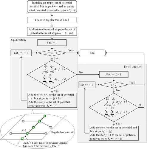
The regular transit often offers an efficient way to serve high demand areas. We consider shortening a bus line when the ridership of the segments ($d_{lj{j}^{\mathrm{\prime }}}$) near the existing terminal stops is low. As shown in Equations (1) and (2), if the ridership of the segment between two sequential bus stops is lower than a threshold value $\delta$ for both directions, then the segment is considered to be removed and the bus stops can be set as potential terminal stops. The generation process is shown in Figure 2. For realism, only bus stops that satisfy certain physical conditions are considered. For example, since we cannot remove a segment in the middle of the bus line, the process can be conducted from the existing terminal stops of both directions, as shown in the shadowed area of Figure 2. Please note that the number of potential terminal bus stops generated through this process is made flexible by changing the threshold value $\delta$, which reflects the preference of transit agencies. The higher the $\delta$ value is, the more bus stops are set as potential bus terminals, which leads to a larger solution space. The optimality of the solution can be guaranteed while the computational load is heavy. On the contrary, the lower the $\delta$ value is, the fewer bus stops are set as potential bus terminals. The computational load is light but the optimality of the solution may not be guaranteed. This can be done in principle separately for any analysis period (e.g. resulting in keeping a fixed service during peak period but opting for a flexible service during other periods). (1) $\begin{array}{rl}& \sum _{j^{\mathrm{\prime }\mathrm{\prime }}=j+1}^{|J_l|}\sum _{j^{\mathrm{\prime }}=1}^j{d}_{l{j}^{\mathrm{\prime }}{j}^{\mathrm{\prime }\mathrm{\prime }}}<\delta \end{array}$(1) (2) $\begin{array}{rl}& \sum _{j^{\mathrm{\prime }\mathrm{\prime }}=1}^j\sum _{j^{\mathrm{\prime }}=j+1}^{|J_l|}{d}_{l{j}^{\mathrm{\prime }}{j}^{\mathrm{\prime }\mathrm{\prime }}}<\delta \end{array}$(2)

Figure 2. Process of generating set of potential terminal bus stops for regular transit.

2.3.2. Generating set of potential serving areas for DRT

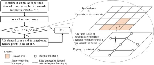
The DRT is expected to be most effective in improving the quality of transit service in low-density areas. Therefore, a demand area is considered to be served by the DRT when the travel time between demand area and bus stop ($t_{ij}^C$) is larger than a threshold value ($\tau$), as shown in Equation (3). Since some regular bus lines may be shortened, the potentially removed bus stops ($j\in S_r$) should be excluded in this step. The flexibility of the formula depends on the threshold value $\tau$, which reflects the preference of transit agencies. The generation process is shown in Figure 3. Please note that the direct neighbouring demand area with at least one regular bus stop is also included in the potential serving areas set to provide a good transfer condition between the DRT and the regular transit. (3) $\begin{array}{r}\begin{array}{cc}{t}_{ij}^C>\tau ,& i\in I;j\in J\mathrm{\setminus }{S}_r\end{array}\end{array}$(3)

Figure 3. Process of generating set of potential serving areas for DRT.

2.4. Optimisation model

The model is to optimise the setting of terminal bus stops for the regular transit, the serving demand areas for the DRT, and the allocation of the fleet size to both services. Since the passenger assignment problem is reduced to a shortest path problem, it can be directly calculated if the design scheme is given without iteration. Consequently, the proposed model can be considered as a single level model. The passenger flow assignment is regarded then as one of the optimisation constraints.

2.4.1. Objective function

The optimisation program considers the total travel time of passengers ($T$) and the total fleet size (represented by the number of vehicles, $C$) of transit lines, as shown in the first and second terms in Equation (4), respectively. The total fleet size is converted into units of time by introducing the weight factor $\alpha$. (4) $\begin{array}{r}\underset{g_l^s,g_l^e,{\beta }_i,m_l^B,m^R}{min}T+\alpha C\end{array}$(4)

2.4.2. Constraints

1. Total passenger travel time ($T$)

The total travel time can be calculated by the sum product of passenger demand ($d_{i{i}^{\mathrm{\prime }}}$) and the corresponding travel times ($T_{i{i}^{\mathrm{\prime }}}$) for each passenger demand pair, as shown in Equation (5). $d_{i{i}^{\mathrm{\prime }}}$ is an input parameter. $T_{i{i}^{\mathrm{\prime }}}$ can be obtained from the passenger flow assignment. (5) $\begin{array}{r}T=\sum _{(i,i^{\mathrm{\prime }})}{d}_{i{i}^{\mathrm{\prime }}}{T}_{i{i}^{\mathrm{\prime }}},\mathrm{\forall }i,i^{\mathrm{\prime }}\in I\end{array}$(5)

1. Setting edges’ weights

The weight of the edge connecting bus stops that belong to the same regular bus line ($w_{j{j}^{\mathrm{\prime }}}$) equals to the sum of the travel time of regular transit between bus stops ($t_{j{j}^{\mathrm{\prime }}}^B$) and the waiting time for regular transit ($u_{j{j}^{\mathrm{\prime }}}^B$), as shown in Equation (6). $t_{j{j}^{\mathrm{\prime }}}^B$ is an input parameter. $u_{j{j}^{\mathrm{\prime }}}^B$ can be calculated by Equation (10). (6) $\begin{array}{r}\begin{array}{c}{w}_{j{j}^{\mathrm{\prime }}}=t_{j{j}^{\mathrm{\prime }}}^B+u_{j{j}^{\mathrm{\prime }}}^B,\mathrm{\forall }j,j^{\mathrm{\prime }}\in J_l\end{array}\end{array}$(6)

The weight of the edge connecting bus stops that belong to the different regular bus line ($w_{j{j}^{\mathrm{\prime }}}$) represents the penalty time of the transferring ($t_r$), which account for the discomfort associated with transferring, as shown in Equation (7). Please note only these bus stops can achieve transferring will be set. (7) $\begin{array}{r}\begin{array}{c}{w}_{j{j}^{\mathrm{\prime }}}=t_r,\mathrm{\forall }j\in J_l;j^{\mathrm{\prime }}\in J_{l^{\mathrm{\prime }}}\end{array}\end{array}$(7)

The weight of the edge connecting demand areas and regular bus stops ($w_{ij}$) equals to the travel time between demand area and bus stop ($t_{ij}^C$), as shown in Equation (8). (8) $\begin{array}{r}\begin{array}{c}{w}_{ij}=t_{ij}^C,\mathrm{\forall }i\in I;j\in J\end{array}\end{array}$(8)

The weight of the edge connecting demand areas equals to the travel time of DRT between demand areas ($t_{i{i}^{\mathrm{\prime }}}^R$) and the waiting time for DRT ($u_{i{i}^{\mathrm{\prime }}}^R$). $t_{i{i}^{\mathrm{\prime }}}^R$ can be determined by solving the travelling salesman problem based on graph theory, which will be explained in Equation (13). $u_{i{i}^{\mathrm{\prime }}}^R$ can be calculated by Equation (11). (9) $\begin{array}{r}\begin{array}{c}{w}_{i{i}^{\mathrm{\prime }}}=t_{i{i}^{\mathrm{\prime }}}^R+u_{i{i}^{\mathrm{\prime }}}^R,\mathrm{\forall }i,i^{\mathrm{\prime }}\in I\end{array}\end{array}$(9)

1. Passenger waiting time

The average waiting time for regular transit ($u_{j{j}^{\mathrm{\prime }}}^B$) is determined by the sum of the frequencies of bus lines that serve the stop pairs. The waiting time for a bus line is on average equal to half its frequency in cases of random arrivals (Osuna and Newell 1972) for which passengers do not bother coordinating their arrival times with service arrival times. If more than one bus line serves a stop pair, the passenger can take the bus of any bus line that arrives first. Therefore, the average waiting time for regular transit is equal to half of the sum of the headways of bus lines that serve the stop pair (i.e. hence determined by the sum of the frequencies), as shown in Equation (10). Please note the waiting time can be reduced if the passengers have the information on bus arrivals, i.e. the schedule of the bus line. The headway $h_l^B$ can be calculated by Equation (12). Since the cost of a unit of waiting time is higher than that of the in-vehicle time and access time (Hossain, Hunt, and Wirasinghe 2015; Nuzzolo and Comi 2016; Ansari Esfeh et al. 2020), the penalty factor ${\gamma }_t$ reflects the equivalent time of the waiting time against the in-vehicle time. (10) $\begin{array}{r}{u}_{j{j}^{\mathrm{\prime }}}^B=\frac{{\gamma }_t}{2}{\left[\sum _l\frac{1}{h_l^B}\right]}^{-1},\mathrm{\forall }j,j^{\mathrm{\prime }}\in J_l\end{array}$(10)

The average waiting time for DRT ($u_z^R$) is determined by the availability of DRT served in the area, as shown in Equation (11). The headway $h_z^R$ can be calculated by Equation (13). Since the vehicle scheduling of the DRT is more flexible than the regular transit, we use the coefficient ${\gamma }_w$ to reflect the operation level of the DRT. If the operation of the DRT is well managed, the waiting time for DRT should be low, which can be reflected by setting a low value of ${\gamma }_w$. Otherwise, the value of ${\gamma }_w$ should be high to reflect a poorly managed DRT service. This allows reflecting the impact of service dynamics on its macroscopic service performance level. (11) $\begin{array}{r}{u}_z^R=\frac{{\gamma }_w}{2}{h}_z^R,\mathrm{\forall }z\in Z\end{array}$(11)

1. Relationship among the headway, trip duration and fleet size

The fleet size required ($m_l^B$ and $m^R$) equals to the trip duration of the line divided by the headway, as shown in Equations (12) and (13) for regular transit and DRT, respectively. (12) $\begin{array}{rl}& m_l^B=\frac{t_l^B}{h_l^B},\mathrm{\forall }l\in L\end{array}$(12) (13) $\begin{array}{rl}& m^R=\frac{t^R}{h^R},\mathrm{\forall }z\in Z\end{array}$(13)

For regular transit (see Equation (12)), the adjusted fleet size of a regular bus line ($m_l^B$) is a decision variable. The trip duration of regular bus lines ($t_l^B$) can be calculated by the travel time between the adjusted start and end bus stops, as shown in Equation (14). (14) $\begin{array}{r}\begin{array}{c}{t}_l^B=t_{g_l^s{g}_l^e}^B+t_{g_l^e{g}_l^s}^B,\mathrm{\forall }l\in L;g_l^s\in J_l;g_l^e\in J_l\end{array}\end{array}$(14)

The average headway can be estimated according to the average trip duration and the fleet size, as shown in Equation (13). Since the DRT service is a flexible operation mode that can dynamically match supply and demand, a DRT bus may not need to pass all the demand areas served by DRT. Therefore, the trip duration is variable. The average trip duration is estimated by the weighted trip durations of all possible routes, as shown in Equation (15). The trip duration of a DRT route ($t_z^R$) can be determined by the travelling salesman problem (TSP). The weight is set as the occurrence possibility of the route, which is related to the OD demand, as shown in Equation (16). In Equation (16), $P_i(A(T)\ge 1)$ represents the probability that the required traffic demand is no less than 1 in a time period $T$. The time period $T$ can be determined by the maximum trip duration divided by the fleet size of the DRT, as shown in Equation (17). (15) $\begin{array}{rl}{t}^R& =\sum _{z\in Z}{P}_z^R{t}_z^R\end{array}$(15) (16) $\begin{array}{rl}{P}_z^R& =\prod _{i\in Z}{P}_i(A(T)\ge 1)\prod _{i\in \overline{Z}}(1-P_i(A(T)\ge 1))\end{array}$(16) (17) $\begin{array}{rl}T& =\frac{\text{max}(t_z^R)}{m^R},\mathrm{\forall }z\in Z\end{array}$(17)

1. Determination of total fleet size of transit lines ($C$)

The total fleet size is expressed as a function of the fleet size, as shown in Equation (18). The fleet size coefficient of the DRT (${\gamma }_c$) is applied to reflect the operation level of the DRT. If the operation of the DRT is well managed, the fleet size coefficient is low. Otherwise, the fleet size coefficient of the DRT (${\gamma }_c$) is high. (18) $\begin{array}{r}C=\sum _l{m}_l^B+{\gamma }_c{m}^R\end{array}$(18)

1. Overcrowding constraint

To ensure an acceptable quality of service, overcrowding is prohibited. The passenger demand using each transit line should hence be no more than the vehicle capacity ($K^B$ and $K^R$), as shown in Equations (19) and (20) for regular transit and DRT, respectively. (19) $\begin{array}{rl}& d_{lj{j}^{\mathrm{\prime }}}{h}_l^B\le K^B,\mathrm{\forall }l\in L;j,j^{\mathrm{\prime }}\in J\end{array}$(19) (20) $\begin{array}{rl}& d_{zi{i}^{\mathrm{\prime }}}{h}_z^R\le K^R,\mathrm{\forall }z\in Z;i,i^{\mathrm{\prime }}\in I\end{array}$(20)

1. Fleet size constraint

The total fleet size to be assigned to the regular transit ($m_l^B$) and DRT ($m^R$) is constrained by an upper bound ($N$) set by the transit agency, e.g. the initial fleet size, as shown in Equation (21). (21) $\begin{array}{r}\sum _l{m}_l^B+{\gamma }_c{m}^R\le N\end{array}$(21)

Moreover, the adjusted fleet size of each regular bus line ($m_l^B$) should not be larger than its original fleet size ($n_l^B$), as shown in Equation (22). (22) $\begin{array}{r}\begin{array}{c}{m}_l^B\le n_l^B,\mathrm{\forall }l\in L\end{array}\end{array}$(22) (8) Passenger flow assignment

The passenger flow assignment to obtain the passenger volume using each transit line. Since the effect of the passenger volume on the travel time is not considered in this transit network design problem, e.g. longer dwelling time at the bus stop, the passenger assignment problem is reduced to a shortest path problem in the designed transit network.

The vertices ($V$) contain demand areas and regular bus stops: $V=I\cup J$. The edges ($E$) contain regular bus lines that connect bus stops ($e_{j{j}^{\mathrm{\prime }}}$), edges connecting demand areas and regular bus stops ($e_{ij}$), and demand-responsive service connecting demand areas ($e_{i{i}^{\mathrm{\prime }}}$). The weights of the edges are the travel time, which are $w_{j{j}^{\mathrm{\prime }}}$, $w_{ij}$, and $w_{i{i}^{\mathrm{\prime }}}$ for the three types of edges, respectively. They are calculated by Equations (6)–(9). The in-vehicle travel time, the waiting time at the bus stops (including the transfer time), and the walking time between demand areas and bus stops are taken into consideration. The parameters that reflect the difference between the regular transit and DRT in travel time are shown in Table 2. The problem is solved by the Dijkstra's algorithm. It is a graph search algorithm that determines the shortest path through a greedy search strategy. In addition, it guarantees the optimal result for the shortest path from a specified vertex to every other vertex in the graph.

Table 2. Parameters reflecting the difference between the two types of transit service.

Items	Difference in travel time	Related parameters
In-vehicle travel time	It depends on the setting of bus lines and their travel time.	$t_{j{j}^{\mathrm{\prime }}}^B$, $t_{i{i}^{\mathrm{\prime }}}^R$
Walking time	Regular transit passengers need to walk between the demand areas and bus stops while DRT passengers have negligible walking times.	$t_{ij}^C$
Waiting time	Regular transit has a longer waiting time at bus stops under the same service frequency conditions.	${\gamma }_w$

3. Solution approach

For the proposed optimisation framework, the solution space is narrowed to an acceptable range through the optimisation preparation step. Here, a boundary-start-based two-step heuristic algorithm is proposed to optimise the combined regular and DRT network. As illustrated in Figure 4, the main idea of the proposed heuristic is to start the search by defining the two following boundaries: (1) the largest catchment area served by regular transit (initial regular transit network) and the smallest catchment area served by DRT; (2) the largest catchment area served by DRT and the smallest catchment area served by regular transit (eliminating all the potential removed bus stops). The flowchart for the solution procedure is illustrated in Figure 5. The iterative optimisation procedure comprises two searching steps, as detailed below.

Figure 4. Main idea of the optimisation procedure.

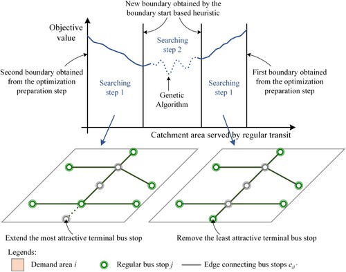
Figure 5. Flowchart for the solution procedure.

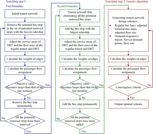
3.1. Searching step 1: boundary-start searching

In step 1, we approach the optimal result from two boundaries. The first boundary is the initial regular transit network. From this boundary, the terminal bus stop in the set of potential removed stops with the lowest ridership will be removed. Correspondingly, the demand area is served by the DRT if the travel time between the relevant demand area and bus stop is larger than a certain threshold value $\tau$. The fleet size of the regular transit is adjusted with the principle of maintaining the original headway. To maintain the second item of the objective function (total fleet size) unchanged, the reduced fleet size of the regular transit is reassigned to the DRT. Therefore, the fleet size of the DRT equals $(n_l^B-m_l^B)/{\gamma }_c$. This procedure is repeated until the value of the objective function becomes larger than that of the last iteration or all the potential removed stops have been removed.

The second boundary is set by the transit network that removes all the potential removed stops in the optimisation preparation step. From this boundary, the bus stop with the largest ridership will be added. Correspondingly, the service areas of DRT and the fleet sizes of the regular transit and DRT are also adjusted, adhering to the same principle of the iteration from the first boundary. This procedure is repeated until the value of the objective function becomes larger than that of the last iteration.

Consequently, we get two new boundaries with a limited number of potential terminal bus stops and potential demand areas. The solution space can be narrowed.

3.2. Searching step 2: genetic algorithm

In step 2, we employ a Genetic Algorithm (GA) (Zhao, Liu, and Li 2016; Ren, Zhao, and Zhou 2021) to further optimise the line setting and fleet size allocation. Specifics on each module of the algorithm are illustrated as follows:

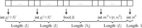
1. The layout variables. An integer code is applied in this study. The string, which represents a transit network design scheme, is structured as shown in Figure 6. The adjusted start and end bus stops, the binary variables to determine the demand areas served by the DRT, the adjusted fleet size of regular bus lines, and the fleet size of DRT are generated.

2. Fitness evaluation. The value of the objective function is regarded as the fitness score of a chromosome.

3. Selection. A new population is bred by using a binary tournament selection method (Cheng 1999) according to the fitness of each chromosome. Tournament selection runs a ‘tournament’ among a few individuals chosen at random from the population and selects the one with the best fitness.

4. Crossover. A uniform crossover operator is used. The genes of two paired individuals are exchanged with the same crossover probability, thus forming two new individuals. The crossover probability is set to 0.25.

5. Mutation. A uniform mutation is used. Uniform Mutation uses random numbers within a certain range to replace the original gene value with a small probability. The mutation probability is set to 0.01.

6. Stopping criteria. In each iteration, the crossover and mutation operations are performed on the chromosomes to generate new solution populations. This procedure is repeated until the difference between the best fitness of two adjacent iterations is less than a pre-defined threshold $\epsilon$, which is set to 0.001. Moreover, the stability of GA somehow relies on the convergence criteria. The stricter the convergence criteria, the more stable the result will be. In the case study, we find that the optimal solution can usually be obtained after around 100 iterations. To avoid the local optimisation caused by the randomness of genetic algorithm, the least number of iterations is set to be 300.

Figure 6. String of the solution.

4. Case study

An area with 36 passenger demand zones, 5 regular bus lines, and 25 regular bus stops is used as an example to test the plausibility of the proposed model, as shown in Figure 7. The input data are shown in Table 3.

Figure 7. Passenger demand zones and original transit network of the case study.

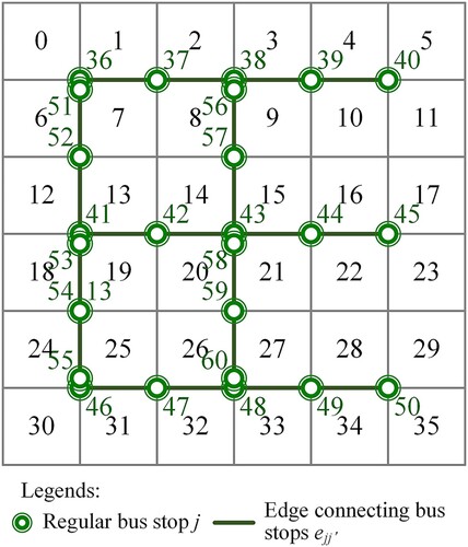
Table 3. Input data of the case study.

Input parameters	Values
Set of demand areas	$I=\{0,1,\dots ,35\}$
Set of regular bus stops	$J=\{36,37,\dots ,60\}$
Set of regular bus lines	$L=\{1,2,3,4,5\}$
Initial fleet size of regular bus line $l$, vehicles	$n_l^B=\{5,5,5,5,5\},\mathrm{\forall }l\in L$
Fleet size limits, vehicles	$N=50$
Set of bus stops of line $l$ in a sequential order	$J_1=\{36,\dots ,40\}$, $J_2=\{41,\dots 45\}$, $J_3=\{46,\dots ,50\}$, $J_4=\{51,\dots ,55\}$, $J_5=\{56,\dots ,60\}$
Travel time of regular transit from bus stop $j$ to bus stop $j{}^{\mathrm{\prime }}$, h	$t_{j{j}^{\mathrm{\prime }}}^B=1/12$ for the neighbouring bus stops
Travel time between demand area $i$ and bus stop $j$, h	$t_{ij}^C=1/10$ for the bus stop $j$ besides the demand area $i$, otherwise, 1/4 h are added for crossing one passenger demand zone
Travel time of DRT between demand areas $i$ and $i{}^{\mathrm{\prime }}$, h	$t_{i{i}^{\mathrm{\prime }}}^R=1/15$ for crossing one demand zone
Penalty time for the transferring	$t_r=1/120$
Passenger demand from demand area $i$ to demand area $i{}^{\mathrm{\prime }}$, person/h	$d_{i{i}^{\mathrm{\prime }}}=10,\mathrm{\forall }i,i^{\mathrm{\prime }}\in I\mathrm{\setminus }\{5,11,17,23,29,35\};i\ne i^{\mathrm{\prime }}$$d_{i{i}^{\mathrm{\prime }}}=1\mathrm{\forall }i\in \{5,11,17,23,29,35\},i^{\mathrm{\prime }}\in I;i\ne i^{\mathrm{\prime }}$$d_{i{i}^{\mathrm{\prime }}}=0,\mathrm{\forall }i{i}^{\mathrm{\prime }}\in I;i=i^{\mathrm{\prime }}$
Vehicle capacity for regular transit and DRT, person/veh	$K^B=60$, $K^R=30$
Weight factor that convert the fleet size into units of time	$\alpha =20$
Penalty factor for the waiting time	${\gamma }_t=1.1$
Equivalent factor that convert the fleet size of DRT into that of the regular transit	${\gamma }_c=0.5$
Threshold upon which a bus stop can be considered to be removed, person/h	$\delta =60$
Threshold upon which a demand area can be considered to be served by the DRT, h	$\tau =1/4$
Threshold value of the stopping criteria in GA	$\epsilon =0.001$

4.1. Optimisation process and results

The original service network design and passenger flow distribution for regular bus lines are shown in Figure 8. The value of the objective function is 4557 passenger-hours. We generate potential terminal bus stops for regular transit and the potential service zones for DRT based on the ridership of the bus lines in the optimisation preparation step. The regular bus line may be shortened when the ridership of the segments near the existing terminal stops are low, while the demand area may be served by the DRT when the travel time between demand area and bus stop is larger. The results of the optimisation preparation are shown in Table 4.

Figure 8. Original passenger demand flow distribution on regular bus lines.

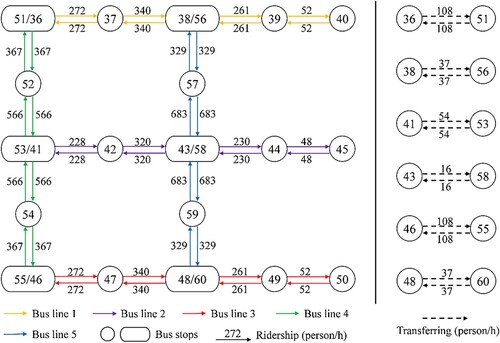
Table 4. Potential terminal bus stops and service zones.

Items	Results
Set of potential start bus stops for regular transit	$S_l^s=[36,41,46,51,56]$
Set of potential end bus stops for regular transit	$S_l^e=[39,40,44,45,49,50,55,60]$
Set of potential service zone for demand-response transit	$S_d=[4,5,10,11,16,17,22,23,28,29,34,35]$

Next, we carry out the optimisation. The design schemes (the layout of the transit network and the fleet size) at each optimisation step are shown in Figure 9. The convergence and computational time are shown in Figure 10. The total travel time of passengers and the total fleet size of transit lines are 3806 h and 20.5 vehicles (16 regular buses and 9 DRT buses), respectively. The objective value of the optimal scheme is 4216 h.

Figure 9. Design schemes at each optimisation step.

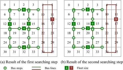
Figure 10. Convergence and computational time of the case study.

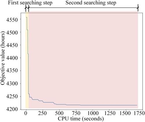
In the first searching step, the feasible region is reduced from the two boundaries, while the optimal result is obtained in the subsequent searching step with the consideration of various combinations. One can find that a sub-optimal solution (objective value = 4302, 74.78% of the optimal scheme) can be quickly (46 s, 2.76% of the total optimisation time) found by applying the first searching step. As shown in Figure 9(a), the three horizontal regular bus lines (lines 1, 2, and 3) with low ridership are shortened. Meanwhile, the low-density areas (the right two columns of demand areas) are served by the DRT service. It indicates that replacing the regular transit lines by the DRT service in low-density areas can help in improving the operational effectiveness of transit service. Notwithstanding, in the second searching step, a better solution (objective value = 4216) can be obtained, yet only after spending a considerably higher computational time (1621 s), using a heuristic algorithm (Figure 10). From Figure 9, One can observe that the overall structure of the regular transit and DRT network remains the same as the one obtained at the end of the first searching step. The service-specific fleet sizes are optimised. More vehicles are assigned to the DRT compared to the result of the first searching step.

4.2. Optimisation effectiveness analysis

To evaluate the effectiveness of the proposed model, three comparison analyses are conducted.

1. Evaluation of the effectiveness of the optimisation preparation step. An optimisation result without the optimisation preparation step was added for comparison. As shown in Table 5, the same optimisation result can be obtained with and without the optimisation preparation step. However, the computational time can be greatly reduced (∼88%) using the proposed optimisation preparation step.

2. Evaluation of the effectiveness of the boundary-start searching step. An optimisation result without the boundary-start searching step (searching step 1) was added for comparison. As shown in Table 6, the same optimisation result can be obtained with and without the boundary-start searching step. However, the computational time can be reduced (∼60%) using the proposed boundary-start searching step.

3. Evaluation of the effectiveness of the joint optimisation. Two single-side optimisation results, i.e. only regular transit and only DRT, were added for comparison. The results are shown in Table 7. Although single-side optimisations can reduce the objective value comparing to the original transit network, there is a certain gap (∼7% in this small case study) when compared with the joint optimisation scheme.

Table 5. Comparison with the optimisation method without the preparation step.

Method	Objective value (h)	CPU time (s)
With preparation (proposed model)	4216	1667
Without preparation	4216	14,153

Table 6. Comparison with the optimisation method without boundary-start searching step.

Method	Objective value (h)	CPU time (s)
With boundary-start searching (proposed model)	4216	1667
Without boundary-start searching	4216	4145

Table 7. Comparison with two single-side optimisations.

Method	Objective value (h)	Travel time (h)	Fleet size (vehicles)
Joint optimisation	4216	3806	20.5
Only regular transit	4496	4146	17.5
Only DRT	4557	4047	25.5

4.3. Sensitivity analysis

The optimal scheme depends on many influencing factors. This section discusses the passenger travel time and fleet size change with respect to the model parameters, including the preference of the decision maker (reflected by $\alpha$), the operation level for demand-response transit (reflected by ${\gamma }_w$), the threshold value of ridership upon which a bus stop can be considered to be removed ($\delta$), and the travel time of DRT between demand areas ($t_{i{i}^{\mathrm{\prime }}}^R$).

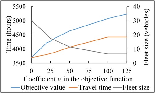
The fleet size coefficient (α) reflects the preference of the decision maker in relation to objective function’s components. When the decision maker attaches greater importance to the level of service of passengers as compared to operational costs, lower values of α should be set. Otherwise, higher values of α should be set. This coefficient expresses the trade-off made between two different objective function components, allowing for the consideration of a single compensatory function. Different decision makers may have different preferences and our formulation can directly accommodate those. As shown in Figure 11, with the coefficient $\alpha$ increasing from 0 (totally neglecting the fleet size) to 125 (a very high weight on the fleet size), the total travel time of passengers increases from 3697 to 4425 h, the total fleet size decreases from 60 vehicles to 6.5 vehicles, and the objection function value increases from 3697 to 5238 h. It makes sense that the optimal scheme changes from deploying the maximum fleet size to using a rather small fleet since the trade-off within the objective function value shifts from maximising passenger level-of-service to focusing on fleet size-minimisation.

Figure 11. Effect of the time-fleet size coefficient $\alpha$.

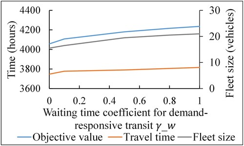
The operation level of the DRT, which is reflected using the waiting time coefficient and fleet size coefficient for DRT, can affect the performance of the transit network. As shown in Figure 12, with the waiting time coefficient for DRT ${\gamma }_w$ increasing from 0 (no waiting time for DRT, which represents the well-organised operation of DRT) to 1 (the waiting time for DRT is equal to the regular transit, which represents the badly organised operation), the total travel time of passengers increases from 3747 to 3816 h, and the objection function value increases from 4057 to 4236 h. The reduction of the operational management level of the DRT leads to an increase in the travel time of passengers. For those who use the DRT, the travel time increases from 1064 to 1487 h (42%). However, since the DRT only serves the area with low passenger demand in this case study, the increase in total travel time is fairly small (4.4%).

Figure 12. Effect of the waiting time coefficient for DRT ${\gamma }_w$.

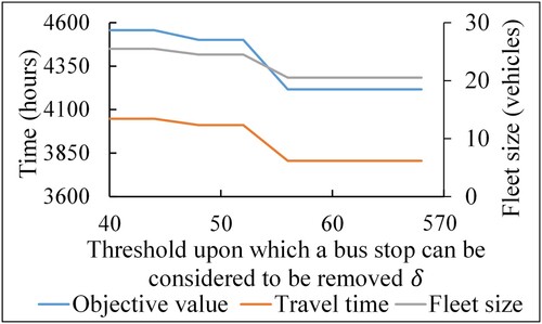
The parameter $\delta$ is a threshold value for the ridership upon which a bus stop can be considered to be removed. More bus stops will be selected as potential removed stops when a higher value of the threshold is set. Since the highest sectional passenger volume in the case study network is 566, threshold $\delta$ values ranging between 40 and 570 are examined. As shown in Figure 13, as the threshold $\delta$ continues to increase, the objective value is reduced to the optimal value. In the case study, when the threshold is less than 48, no stops are considered to be removed. The objective value is 4557 h. With an increase of $\delta$, the solution space expands. This analysis further indicates that setting $\delta =60$ in Section 4.1 is appropriate.

Figure 13. Effect of the threshold $\delta$.

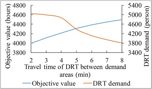
Travel time is a critical determinant of passengers’ travel path choice. Figure 14 presents the effect of DRT’s travel time between demand areas ($t_{i{i}^{\mathrm{\prime }}}^R$) on the demand for this service as well as the objective function value. With the travel time of DRT between demand areas increasing from 0.5 to 2 times of the original setting, the total travel time of passengers increases from 3994 to 4493 h, and the DRT demand decreases from 5054 to 3798 passengers. DRT is more attractive than the regular transit when $t_{i{i}^{\mathrm{\prime }}}^R$ is very low whereas when $t_{i{i}^{\mathrm{\prime }}}^R$ is high only passengers within the areas that are not covered by the regular transit will use the DRT.

Figure 14. Effect of the travel time of DRT.

Moreover, it is interesting to note that the variations in the waiting time coefficient and fleet size coefficient for DRT do not change the service area of the DRT in the case study. The transit network maintains an overall high level of performance by replacing the regular transit in low demand area with DRT. The difference among the design schemes lies in the fleet size assigned to different services.

5. Conclusions

This study proposed a joint optimisation model of regular and DRT networks. The terminal (start/end) bus stops of regular bus lines, the service area of the DRT, and the fleet size of both regular transit and DRT are optimised simultaneously with the objective of minimising the total travel time of passengers and the total fleet size. To obtain a reasonable design scheme and to reduce the computational load, a rule-based optimisation preparation process is added. A tailored boundary-start-based two-step heuristic algorithm is proposed to solve the model. The results of the numerical analysis show the following:

1. The optimisation preparation process and the tailored heuristic algorithm can effectively find a reasonable solution. The proposed model found a sub-optimal solution (75% of the optimal scheme) in a relevantly short time, and is also able to obtain the (globally) optimal scheme after spending a considerably longer computational time.

2. The performance of the mixed regular and DRT network will be affected by the preference of the decision-maker (reflected by $\alpha$) and the operational properties of the DRT service (reflected by ${\gamma }_w$ and ${\gamma }_c$). A reduction in the operational level of the DRT results in a considerable increase in the travel time of DRT passengers. However, since the DRT only serves the area with low passenger demand in this case study, the increase in total travel time of passengers remains limited (4.4%).

In our problem formulation, we assumed that there is a regular transit network in place in the study area. The regular bus lines can be shortened, and the fleet size can be reduced, but the regular bus line can neither be extended nor a new line can be added. Since the removal of middle stops is not considered in this study, the model cannot deal adequately with the case of ring routes. Moreover, future studies can be carried out to extend the all-or-nothing assignment in the passenger flow assignment problem to user-equilibrium and apply the model in a large-scale network to examine the scalability of the proposed approach.

Disclosure statement

No potential conflict of interest was reported by the author(s).

Additional information

Funding

The first author was supported by the National Natural Science Foundation of China [grant numbers 71971140 and 72011530439]. The third author was supported by the CriticalMaaS project [grant number 804469], which is financed by the European Research Council and Amsterdam Institute for Advanced Metropolitan Solutions.

References

- Alonso-González, M. J., S. Hoogendoorn-Lanser, N. van Oort, O. Cats, and S. Hoogendoorn. 2020. “Drivers and Barriers in Adopting Mobility as a Service (MaaS) – A Latent Class Cluster Analysis of Attitudes.” Transportation Research Part A: Policy and Practice 132: 378–401.
- Ansari Esfeh, M., S. Wirasinghe, S. Saidi, and L. Kattan. 2020. “Waiting Time and Headway Modelling for Urban Transit Systems – A Critical Review and Proposed Approach.” Transport Reviews 41 (2): 141–163.
- Arbex, R. O., and C. B. da Cunha. 2015. “Efficient Transit Network Design and Frequencies Setting Multi-Objective Optimization by Alternating Objective Genetic Algorithm.” Transportation Research Part B: Methodological 81: 355–376.
- Basu, R., A. Araldo, A. P. Akkinepally, B. H. Nahmias Biran, K. Basak, R. Seshadri, N. Deshmukh, N. Kumar, C. L. Azevedo, and M. Ben-Akiva. 2018. “Automated Mobility-on-Demand vs. Mass Transit: A Multi-Modal Activity-Driven Agent-Based Simulation Approach.” Transportation Research Record 2672 (8): 608–618.
- Byrne, B. F., and V. R. Vuchic. 1972. “Public Transportation Line Positions and Headways for Minimum Cost.” Traffic Flow and Transportation 1972: 347–360.
- Calderón, F., and E. J. Miller. 2020. “A Literature Review of Mobility Services: Definitions, Modelling State-of-the-Art, and Key Considerations for a Conceptual Modelling Framework.” Transport Reviews 40 (3): 312–332.
- Ceder, A. 2007. Public Transit Planning and Operation: Theory, Modelling and Practice. Oxford: Elsevier.
- Coutinho, F. M., N. van Oort, Z. Christoforou, M. J. Alonso-González, O. Cats, and S. Hoogendoorn. 2020. “Impacts of Replacing a Fixed Public Transport Line by a Demand Responsive Transport System: Case Study of a Rural Area in Amsterdam.” Research in Transportation Economics 80: 100910.
- Daganzo, C. F., and Y. Ouyang. 2019. “A General Model of Demand-Responsive Transportation Services: From Taxi to Ridesharing to Dial-a-Ride.” Transportation Research Part B: Methodological 126: 213–224.
- Desaulniers, G., and M. D. Hickman. 2007. “Public Transit.” Handbooks in Operations Research and Management Science 14: 69–127.
- Diana, M., L. Quadrifoglio, and C. Pronello. 2007. “Emissions of Demand Responsive Services as an Alternative to Conventional Transit Systems.” Transportation Research Part D: Transport and Environment 12 (3): 183–188.
- Franco, P., R. Johnston, and E. McCormick. 2020. “Demand Responsive Transport: Generation of Activity Patterns from Mobile Phone Network Data to Support the Operation of New Mobility Services.” Transportation Research Part A: Policy and Practice 131: 244–266.
- Gen, M., and Cheng R. 1999. Genetic Algorithms and Engineering Optimization. New Jersey: John Wiley & Sons Inc.
- Gkiotsalitis, K. 2021. “Stop-skipping in Rolling Horizons.” Transportmetrica A: Transport Science 17 (4): 492–520.
- Gkiotsalitis, K., Z. Wu, and O. Cats. 2019. “A Cost-Minimization Model for Bus Fleet Allocation Featuring the Tactical Generation of Short-Turning and Interlining Options.” Transportation Research Part C: Emerging Technologies 98: 14–36.
- Guihaire, V., and J.-K. Hao. 2008. “Transit Network Design and Scheduling: A Global Review.” Transportation Research Part A: Policy and Practice 42 (10): 1251–1273.
- Holroyd, E. 1967. “The Optimum bus Service: A Theoretical Model for a Large Uniform Urban Area.” In Third International Symposium on the Theory of Traffic Flow, 308–328. New York: Elsevier Science.
- Hossain, M. S., J. D. Hunt, and S. Wirasinghe. 2015. “Nature of Influence of Out-of-Vehicle Time-Related Attributes on Transit Attractiveness: A Random Parameters Logit Model Analysis.” Journal of Advanced Transportation 49 (5): 648–662.
- Huang, A., Z. Dou, L. Qi, and L. Wang. 2020. “Flexible Route Optimization for Demand-Responsive Public Transit Service.” Journal of Transportation Engineering Part a-Systems 146 (12): 04020132.
- Ibarra-Rojas, O. J., F. Delgado, R. Giesen, and J. C. Munoz. 2015. “Planning, Operation, and Control of Bus Transport Systems: A Literature Review.” Transportation Research Part B: Methodological 77: 38–75.
- Kepaptsoglou, K., and M. Karlaftis. 2009. “Transit Route Network Design Problem: Review.” Journal of Transportation Engineering 135 (8): 491–505.
- Kim, M. E., J. Levy, and P. Schonfeld. 2019. “Optimal Zone Sizes and Headways for Flexible-Route Bus Services.” Transportation Research Part B: Methodological 130: 67–81.
- Lampkin, W., and P. Saalmans. 1967. “The Design of Routes, Service Frequencies, and Schedules for a Municipal Bus Undertaking: A Case Study.” Journal of the Operational Research Society 18 (4): 375–397.
- Li, X., T. Wang, W. Xu, and J. Hu. 2021. “A Novel Model for Designing a Demand-Responsive Connector (DRC) Transit System with Consideration of Users’ Preferred Time Windows.” IEEE Transactions on Intelligent Transportation Systems 22 (4): 2442–2451.
- Mehran, B., Y. Yang, and S. Mishra. 2020. “Analytical Models for Comparing Operational Costs of Regular Bus and Semi-Flexible Transit Services.” Public Transport 12 (1): 147–169.
- Mendes, L. M., M. R. Bennàssar, and J. Y. Chow. 2017. “Comparison of Light Rail Streetcar Against Shared Autonomous Vehicle Fleet for Brooklyn–Queens Connector in New York City.” Transportation Research Record 2650 (1): 142–151.
- Nuzzolo, A., and A. Comi. 2016. “Advanced Public Transport and Intelligent Transport Systems: New Modelling Challenges.” Transportmetrica A: Transport Science 12 (8): 674–699.
- Oliker, N., and S. Bekhor. 2020. “An Infeasible Start Heuristic for the Transit Route Network Design Problem.” Transportmetrica A: Transport Science 16 (3): 388–408.
- Osuna, E., and G. F. Newell. 1972. “Control Strategies for an Idealized Public Transportation System.” Transportation Science 6 (1): 52–72.
- Pinto, H. K., M. F. Hyland, H. S. Mahmassani, and I. Ö. Verbas. 2020. “Joint Design of Multimodal Transit Networks and Shared Autonomous Mobility Fleets.” Transportation Research Part C: Emerging Technologies 113: 2–20.
- Quadrifoglio, L., R. W. Hall, and M. M. Dessouky. 2006. “Performance and Design of Mobility Allowance Shuttle Transit Services: Bounds on the Maximum Longitudinal Velocity.” Transportation Science 40 (3): 351–363.
- Ren, Y., J. Zhao, and X. Zhou. 2021. “Optimal Design of Scheduling for Bus Rapid Transit by Combining with Passive Signal Priority Control.” International Journal of Sustainable Transportation 15 (5): 407–418.
- Scheltes, A., and G. H. de Almeida Correia. 2017. “Exploring the Use of Automated Vehicles as Last Mile Connection of Train Trips Through an Agent-Based Simulation Model: An Application to Delft, Netherlands.” International Journal of Transportation Science and Technology 6 (1): 28–41.
- Shen, Y., H. Zhang, and J. Zhao. 2018. “Integrating Shared Autonomous Vehicle in Public Transportation System: A Supply-Side Simulation of the First-Mile Service in Singapore.” Transportation Research Part A: Policy and Practice 113: 125–136.
- SuM4All. 2017. Global Mobility Report 2017. Washington, DC: World Bank.
- Szeto, W. Y., and Y. Wu. 2011. “A Simultaneous Bus Route Design and Frequency Setting Problem for Tin Shui Wai, Hong Kong.” European Journal of Operational Research 209 (2): 141–155.
- Wang, Z., J. Yu, W. Hao, J. Tang, Q. Zeng, C. Ma, and R. Yu. 2020. “Two-Step Coordinated Optimization Model of Mixed Demand Responsive Feeder Transit.” Journal of Transportation Engineering Part a-Systems 146 (3): 04019082.
- Wang, Z., J. Yu, W. Hao, and J. Xiang. 2021. “Joint Optimization of Running Route and Scheduling for the Mixed Demand Responsive Feeder Transit with Time-Dependent Travel Times.” IEEE Transactions on Intelligent Transportation Systems 22 (4): 2498–2509.
- Winter, K., O. Cats, G. Correia, and B. van Arem. 2018. “Performance Analysis and Fleet Requirements of Automated Demand-Responsive Transport Systems as an Urban Public Transport Service.” International Journal of Transportation Science and Technology 7 (2): 151–167.
- Yan, S., and H. Chen. 2002. “A Scheduling Model and a Solution Algorithm for Inter-City Bus Carriers.” Transportation Research Part A: Policy and Practice 36 (9): 805–825.
- Zhang, L., T. Chen, B. Yu, and C. Wang. 2021. “Suburban Demand Responsive Transit Service with Rental Vehicles.” IEEE Transactions on Intelligent Transportation Systems 22 (4): 2391–2403.
- Zhao, J., Y. Liu, and P. Li. 2016. “A Network Enhancement Model with Integrated Lane Reorganization and Traffic Control Strategies.” Journal of Advanced Transportation 50 (6): 1090–1110.
- Zhao, J., J. Yu, X. Xia, J. Ye, and Y. Yuan. 2019. “Exclusive bus Lane Network Design: A Perspective from Intersection Operational Dynamics.” Networks and Spatial Economics 19: 1143–1171.
- Zhao, F., and X. Zeng. 2008. “Optimization of Transit Route Network, Vehicle Headways and Timetables for Large-Scale Transit Networks.” European Journal of Operational Research 186 (2): 841–855.