Evaluating the impact of waiting time reliability on route choice using smart card data

ABSTRACT

Unreliable waiting times may cause frustration and anxiety amongst public transport travellers. Although the effect of travel time reliability has been studied extensively, most studies have used stated preferences which have disadvantages, such as an inherent hypothetical bias, or have analysed revealed preferences for road traffic. Here, we derive revealed preferences from passively collected smart card data to analyse the role of waiting time reliability in public transport route choice. We study waiting time reliability as regular and irregular deviations from scheduled values, examining a number of indicators for the latter. Behaviour in morning peak and off-peak hours is contrasted and differences in reliability coefficients for different modes in the network, and for origin and transfer stops are reported. Results from The Hague indicate relatively low reliability ratios with travellers perceiving a 5-minute standard deviation in realised waiting times as an extra 1–5.6 min of planned waiting time.

KEYWORDS:

• Public transport
• waiting time
• reliability
• revealed preferences
• smart card data

1. Introduction

The impact of travel time reliability on route choice behaviour has received much attention in literature. The vast majority of studies have used stated preferences collected through surveys or simulation experiments (Carrion and Levinson 2012; Li, Hensher, and Rose 2010). Due to the costs associated with data collection, only a few have analysed revealed preferences and almost all of these have focussed on car traffic. Fortunately, however, an increasing number of public transport networks are integrated with automatic fare collection (AFC) systems, which enable analysts to glean revealed preferences from this passively collected data. Moreover, automatic vehicle location (AVL) data, provides detailed information on the realised supply characteristics (e.g. travel time, waiting time) of public transport services. In this paper, we combine the revealed preferences from AFC data with reliability information derived from AVL data to establish the role of waiting time reliability in public transport route choice.

Passively collecting revealed preferences offers two important advantages over simulation experiments and conventional stated preferences. First, and most importantly, revealed preferences are free from hypothetical biases that are prevalent in the other methods since observed choices have consequences and are made in real-world situations. Second, passively collecting revealed preferences obviates the need to explicitly convey reliability information, which has proven to be difficult (Bates et al. 2001; Carrion and Levinson 2012). Furthermore, unlike revealed preference questionnaires that enquire about past behaviour, passive data collection allows us to gather significantly more observations. However, since revealed preferences inherently lack experimental control, the amount of information obtained per observation is likely to be significantly lower than stated preferences or simulation experiments. The lack of experimental control could also lead to issues in determining the direction of causality. Privacy regulations may also restrict the amount and type of data that can be used for analysis. Finally, passively collected data typically require significant processing effort and require assumptions regarding attributes that cannot be observed (e.g. Lam and Small 2001; Luo et al. 2018).

While more complete reviews of studies analysing the effect of travel time reliability on travel behaviour are available elsewhere (Carrion and Levinson 2012; Li, Hensher, and Rose 2010), here, we briefly outline those using passively collected data for their analysis. For car traffic, such studies have largely made use of road-pricing experiments in the United States (Alemazkoor, Burris, and Danda 2015; Carrion and Levinson 2013; Lam and Small 2001). This setting offers researchers a unique opportunity to observe choices between a free but (potentially) congested road and a tolled but (almost certainly) uncongested road, and thus, estimate the value of reliability. Travel times and choices are obtained via loop detectors or GPS devices and toll transponders, respectively. In recent years, with the introduction of AFC systems, researchers have used this passively collected data to analyse travel behaviour in public transport systems, often in combination with AVL data. Amongst these studies, for many, general route choice behaviour is the primary aim of the analysis (e.g. Jánošíková, Slavík, and Koháni 2014; Kim et al. 2019). Other studies focus on specific aspects such as, on-board crowding (Hörcher, Graham, and Anderson 2017; Yap, Cats, and van Arem 2020), transfer inconveniences (Guo and Wilson 2011), route choice variability (Kim, Corcoran, and Papamanolis 2017; Kurauchi et al. 2014), or strategic behaviour (Nassir, Hickman, and Ma 2019; Schmöcker, Shimamoto, and Kurauchi 2013). To the best of our knowledge, only Leahy, Batley, and Chen (2016) have used such data to analyse the impact of travel time reliability on route choice behaviour in public transport networks. Our study is different from theirs in two important ways: (i) whereas they evaluate the role of the total trip travel time reliability we focus on and are able to specifically estimate perceptions related to waiting time reliability; and (ii) they use a sample of AFC transactions over the time period under study while we have access to the full population dataset.

In general for the service industry, waiting time is a critical component of satisfaction (Maister 1985). For public transportation too, it has been consistently shown that waiting time has a large impact on behaviour. Unreliability in this important component of travel time may lead to frustration and anxiety amongst travellers. We note that unreliability is inherently an uncertain (Knight 1921) attribute – the true distribution of waiting times is unknown to the travellers. Instead travellers may have their own subjective distributions (Dixit et al. 2019; Meng, Rau, and Mahardhika 2018) that they use to make decisions. However, in line with the majority of previous research on this topic (Carrion and Levinson 2012), we model waiting time unreliability as if it were a known risk. We compare a number of empirical measures of unreliability in our choice analysis. Furthermore, the effects of waiting time unreliability are modelled separately for origin and transfer stations, for different public transport modes, and for morning peak and off-peak hours.

Next, we present our case study: the urban public transport network of The Hague, followed by the methodology outlining data preparation, choice set identification, attribute extraction, and finally choice analysis. We then discuss the estimated choice models and conclude with a summary of the main results and suggest avenues for future work.

2. Case study description

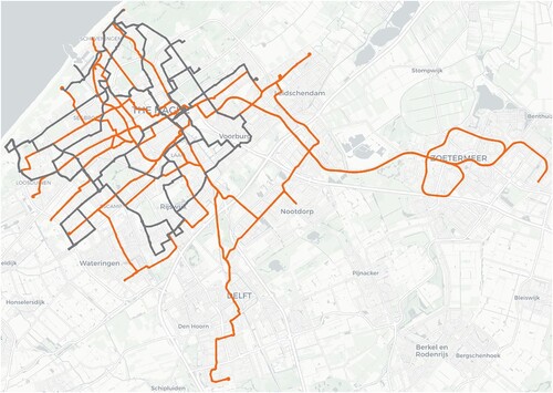
For our analysis, we use smart card data from the urban public transport system in The Hague, the third largest city in the Netherlands. The network contains 12 tram and 8 bus lines connecting 499 aggregated stops (operator-defined ‘parent stations’ in the GTFS data) in The Hague and neighbouring suburbs and towns (Figure 1). About 90% (Yap, Cats, and van Arem 2020) of the trips in the network are paid for through a smart card based AFC system which requires travellers paying with the smart card to interact with the system (i.e. check-in and check-out) upon boarding and alighting a vehicle. Travellers in the network can check scheduled departure times at all tram and bus stops, at most of which, real-time information is also available. For those using mobile internet, real-time information for the entire network is always available.

Figure 1. The Hague tram (orange) and bus (grey) networks in March 2015.

The urban public transport operator in The Hague, HTM, provided us with processed and anonymised AFC and AVL data from March 2015. The provided AFC data consists of journeys constructed by linking individual AFC transactions using a time-based transfer inference method wherein a trip with the same smart card identifier is included in the same journey as the previous trip if the boarding time of the second trip is within 35 min of the alighting time of the first. Since the data we received does not contain these unique identifiers, we are unable to follow individual cards across different journeys. Furthermore, since no information about the type of card or discounts applied is available, segmentation based on such variables is not possible.

The data consists of about 5.9 million inferred journeys and information on boarding and alighting time, stop, and line for each trip in every journey is available. In this study, we analyse and contrast route choice behaviour in weekday morning peak (06:00–09:00) and off-peak (09:00–16:00) hours. After filtering the datasets accordingly and applying the transfer inference procedure (described next), we are left with 1.02 and 2.63 million journeys for the morning peak and off-peak hours, respectively.

3. Methodology

3.1. Data preparation

Three data sources are used: (i) automatic fare collection, (ii) automatic vehicle location, and (iii) general transit feed specification (GTFS) data. While AFC data is the source for behavioural observations, the latter two, being data on the realised and scheduled operations, respectively, provide information on travel time characteristics including waiting time reliability.

To analyse route choice behaviour, complete journeys – as sequences of trips (i.e. rides on a single vehicle) without intervening trip-generating activities – have to be known. Although, the AFC data provided by the operator already consists of journeys, these are inferred by a time-based algorithms which tend to over-estimate the number of transfers (Yap et al. 2017). The time-based algorithm considers two trips to be part of the same journey if the time between the last check-out and next check-in is less than 35 min. Thus, trip-generating activities of shorter duration are ignored, leading to an overestimation of the number of transfers. This is particularly true for an urban public transport system where services have a relatively higher frequency and transfer times are rarely greater than the threshold. Therefore, we apply our own transfer inference algorithm to each journey to check whether the trips linked together by the operator indeed constitute one journey. For this, the AFC and AVL datasets were merged using the technique detailed in Luo et al. (2018).

The transfer inference algorithm is composed of one spatial and one temporal rule. The spatial rule ensures that the alighting stop of one trip and the boarding stop of the next are within 400 Euclidean metres (Yap et al. 2017) of one another. This places an upper bound on the distance travellers will walk to transfer. The temporal rule checks whether, after alighting, the first plausible service (or an earlier one) of the line used in the next trip is boarded. When this is the case, it is unlikely that a traveller will have performed an intermediate trip-generating activity. If the boarding stop is the same as the alighting stop of the previous trip, then the first plausible service is the same as the first service. That is, if the alighting and boarding stops for two consecutive trips are the same, then the first plausible service is the first vehicle of the line (actually) used in the second trip to arrive at the stop after the traveller has alighted. If the two stops are different then it is the first service (of the line used in the next trip) after adding the time required by most people to walk between the two stations. For this, Euclidean distances and a walking speed of 0.66 m/s (Hänseler, Bierlaire, and Scarinci 2016) are used. A slower walking speed is used to ensure that the first plausible service is feasible for the majority (in this case 97.5%) of the population. Note that since it is rare for vehicles in the network to be too crowded for passengers to board, we do not account for the possibility that a traveller does not board the first plausible vehicle due to overcrowding. As an example to understand how the transfer inference algorithm works, consider an operator-inferred journey where a traveller goes from stop A to D, first taking line 1 from A to B, then walking from B to C, and finally taking line 2 from C to D. The traveller alights line 1 at 10:03 and boards line 2 at 10:20. Line 2 departs from C every 10 min (i.e. at 10:00, 10:10, 10:20, etc.) and the distance between stops B and C is 200 m. The transfer thus passes the spatial rule as the distance is less than the threshold of 400 m. Based on the assumed walking speed of 0.66 m/s, the traveller should have arrived at stop C by about 10:05. Thus, the first plausible service of line 2 at stop C is the one at 10:10. Since the traveller instead boarded the service departing at 10:20, it fails the temporal rule and the two trips (A to B and C to D) are separated to two journeys.

Journeys containing transfer between the same lines (about 0.47% of the data) are not removed as long as they pass the above temporal criterion. This is done to accommodate travellers affected by planned and unplanned short-turning, stop-skipping or dead-heading. To avoid considering such routes as different alternatives, wherever the temporal criterion is passed for such transfers, the trips involved are merged into one (thus removing the extra transfer to the same line).

Applying this transfer inference algorithm reduces the number of journeys with at least one transfer from 18.8% of all journeys in the dataset provided by the operator to 10.8%. Journeys with more than one transfer make up about 0.5% of the total.

3.2. Choice set identification

A number of choice set generation methodologies have been proposed in literature. These approaches typically either require enumerating shortest paths or relying on a variety of behavioural assumptions (see Bovy 2009; Prato 2009, for an overview). However, studies analysing travel behaviour using AFC data have typically identified the route choice set for each origin-destination (OD) pair directly from the set of observed routes (Kim et al. 2019; Leahy, Batley, and Chen 2016; Yap, Cats, and van Arem 2020). A potential disadvantage of this method is that we do not include in our analysis routes that are feasible but are only used for a few trips or not at all. However, since the data used for this study covers the entire network and covers a reasonably long period of time, this disadvantage is fairly low and the direct identification method is also suitable for our analysis.

The following filtering rules are applied to identify OD pairs (and associated route alternatives) for choice analysis: (i) each OD pair must have at least 2 route alternatives, (ii) each OD pair must have at least 200 trips between them, and (iii) each route alternative must make up at least 10% of the observations of its OD pair. While the first rule ensures that we are able to observe trade-offs between alternatives, the lower limits on the number of observations ensure that there is sufficient information to estimate behavioural parameters as well as to eliminate unusual observations that do not take place regularly. The set of eligible OD pairs is filtered iteratively using these rules until a stable set is obtained.

For the choice analysis, routes have to be uniquely defined such that travellers can be reasonably expected to perceive one route to be different from another. To this end, route alternatives are defined by the sequence of modes used and the boarding, intermediate and alighting stops. We consider lines (of the same mode) along a common corridor (i.e. traversing the same sequence of stops) to be perceived equivalently by travellers. Moreover, routes that have different transfer stops but are otherwise similar are distinguished as separate alternatives. This is to account for the fact that different stops may be associated with different waiting time reliability characteristics due to various reasons, such as planned transfer coordination.

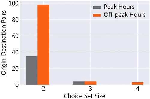
Given these filtering rules, for the morning peak, we are left with 39 OD pairs and 30,606 inferred journeys suitable for choice analysis while for the off-peak, we have 105 OD pairs and 85,952 inferred journeys. As shown in Figure 2, most OD pairs in both time periods have only 2 alternatives.

Figure 2. Choice set size distribution for the morning peak and off-peak hours.

3.3. Choice attributes

Once all eligible OD pairs and associated choice sets are obtained, attribute values for the alternatives are assigned. The following attributes are used for the choice analysis: for each leg of the route, its (i) mode, (ii) in-vehicle time, and (iii) waiting time (and its components: scheduled waiting time, and regular and irregular deviations), and for the route alternative as a whole, its (iv) path size factor (indicating degree of overlap with other alternatives) and the (v) number of transfers. Attributes (i) and (v) – mode used in each leg and number of transfers – are directly known from the route definition. Travel time attributes are aggregated over each hour per day of the week (e.g. Mondays, 0900h–1000 h) to account for the fact that travel time attributes may vary over time. Unfortunately, the data available does not include fare (or discount) information. However, for alternatives of a given OD pair, the price difference is typically in the order of cents. Moreover, paying by smart card may make it even more difficult for passengers to internalise costs. Having said that, we acknowledge that any fare effects will instead show up in the coefficients of other attributes, particularly, in-vehicle time, number of transfers, and mode, which are associated with price differences. We describe each choice attribute and its calculation below.

3.3.1. Modes and number of transfers

The mode used (denoted by m in Equation (3(3) $\begin{array}{rl}V& ={\beta }^{\text{trans}}\cdot n^{\text{trans}}+{\beta }^{\text{ps}}\cdot \ln (p)+\sum _{m\in \text{M}}{\beta }_m^{\text{ivt}}\cdot t_{0,m}^{\text{ivt}}\\ & +\sum _{m\in \text{M}}{\beta }_{0,m}^{\text{owt}}\cdot t_{0,m}^{\text{owt}}+{\beta }_{0,m}^{\text{twt}}\cdot t_{0,m}^{\text{twt}}\\ & +\sum _{m\in \text{M}}{\beta }_{\text{d},m}^{\text{owt}}\cdot t_{\text{d},m}^{\text{owt}}+{\beta }_{\text{d},m}^{\text{twt}}\cdot t_{\text{d},m}^{\text{twt}}\\ & +\sum _{m\in \text{M}}{\beta }_{\text{r},m}^{\text{owt}}\cdot t_{\text{r},m}^{\text{owt}}+{\beta }_{\text{r},m}^{\text{twt}}\cdot t_{\text{r},m}^{\text{twt}}\end{array}$(3) )) helps to understand how travel time components are weighed for different modes by travellers while the number of transfers (n^trans) is used to evaluate the transfer penalty, that is, the additional disutility beyond the transfer waiting time. Amongst the journeys eligible for choice analysis, all have a maximum of one transfer although the vast majority of observations are direct tram trips. Barring two OD pairs in the off-peak hours, whenever a bus-based option is available, it competes against a tram alternative. However, the overall proportion of observations where the choice between bus and tram is observed is also quite low: only 5 (5.12% of observations) and 11 (9.86% of observations) such OD pairs are available in the peak and off-peak hours, respectively. This may be expected given the different functions the two networks perform in a wheel & spoke-like network where the tram lines radiate out of the centre and the bus lines provide peripheral connections.

3.3.2. In-vehicle time

Since the focus here is on waiting time reliability, only scheduled in-vehicle times ($t_m^{\text{ivt}}$) are used in the analysis. In-vehicle times are separately calculated for each stop pair and line combination by taking the mean of the scheduled values over the aggregation period. For common corridors, the in-vehicle times are assigned by taking the median of the in-vehicle times of the individual lines in the corridors.

3.3.3. Waiting time

We use the reduced-form approach to include reliability effects in the route choice model. This method directly introduces statistical measures of travel times in the utility function (Börjesson, Eliasson, and Franklin 2012). Usually, centrality and dispersion of realised travel times are used (Alemazkoor, Burris, and Danda 2015; Carrion and Levinson 2012) with the aim of estimating how expectations of travel times (centrality measures such as mean or median) are traded-off against dispersion parameters (such as standard deviation or skew). However, unlike road traffic, since schedules exist for public transport networks, they may loom large in the decision process. Therefore, based on van Oort et al. (2015) and van Oort (2016), we consider the following waiting time components to quantify the effect of reliability on route choice behaviour: (i) scheduled waiting time ($t_{0,m}^{\text{wt}}$); and (ii) regular deviations ($t_{\text{d},m}^{\text{wt}}$) and (iii) irregular deviations ($t_{\text{r},m}^{\text{wt}}$; where r is replaced by the indicator name) of the realised waiting times from the schedule.

Regular deviations are calculated as the difference between the median of realised and scheduled values. For irregular deviations, a few studies on road traffic have compared indicators (Alemazkoor, Burris, and Danda 2015; Bogers, Van Lint, and Van Zuylen 2008; Bogers et al. 2006) but there is little consensus regarding which dispersion measures best represent the perception of travel time unreliability. van Lint, van Zuylen, and Tu (2008) categorise these measures into (i) statistical ranges, (ii) buffer times, (iii) tardy trip measures, and (iv) probabilistic measures. The first two categories are commonly included in travel behaviour studies: statistical ranges (for instance, variance or standard deviation) measure the variation around the central value while buffer times indicate the extent of worse case scenarios, usually through the difference between the 90th or 95th percentile travel time and the median. In our analysis, we tested absolute and normalised formulations of these two commonly used dispersion measures (Table 1) to evaluate which representations best explain observed behaviour.

Table 1. Waiting time dispersion measures considered.

Category	Statistical measure	Formula
Statistical range	Standard deviation	$\sqrt{{\displaystyle \frac{\sum {(x_i-\mu )}^2}{N}}}$
	Normalised variance (van Lint, van Zuylen, and Tu 2008)	${\displaystyle \frac{p_{90}-p_{10}}{p_{50}}}$
Buffer times	Reliability buffer time	$p_{95}-p_{50}$
	Reliability buffer index	${\displaystyle \frac{p_{95}-p_{50}}{p_{50}}}$
	Normalised skew (van Lint, van Zuylen, and Tu 2008)	${\displaystyle \frac{p_{90}-p_{50}}{p_{50}-p_{10}}}$

For a given time period aggregate (hour-day of week), x_i is the i^th realised value, µ is the mean of realised values, N is the number of realisations, p_m is the m^th percentile of the realised values.

The effects of waiting times at origin ($t^{\text{owt}}$) and transfer ($t^{\text{twt}}$) stops are considered separately. We assume that travellers arrive uniformly at origin stops and subsequently consider half of the headway time (of relevant lines) as the origin waiting time. Previous studies have found that for headways up to 10–12 min, passengers tend to indeed arrive randomly (Ansari Esfeh et al. 2020; Fan and Machemehl 2009; van Oort 2011). Figure 3, top-left shows the distribution of calculated waiting times at origin (the headways are double these values). It can be seen that although our assumption is reasonable for most alternatives, for some, the headways are slightly higher. For these, we may be considering a slightly higher waiting time than reality as we can expect travellers to begin coordinating their arrivals to departure times (or be ‘less random’ Fan and Machemehl (2009)). Furthermore, we assume that travellers take the first vehicle available to them since denied boarding is rare in The Hague (Yap, Cats, and van Arem 2020). Transfer waiting times, on the other hand, can be fully observed as the time between departures of the lines used to and from the transfer stop. However, for alternatives with common corridors, the expected transfer waiting time also depends on the lines used from the previous stop; and therefore ultimately on the assumptions made regarding traveller arrivals at the origin. For example, to obtain the waiting time at the first transfer stop, the proportion of travellers using each line at the origin stop (under given assumptions) is used to weight the feasible transfer times between the lines from the origin to the transfer stop and from the transfer stop onward.

Figure 3. Scheduled, regular deviations, and irregular deviations for origin and transfer waiting times of route alternatives in the choice analysis (in minutes).

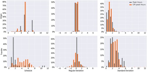
Figure 3 shows the distribution of scheduled waiting times, and regular and irregular deviations for the route alternatives eligible for analysis. (Since it is ultimately selected for the choice models in section 4, only standard deviation is shown here). While the origin waiting times are generally low, transfer waiting times show a stark difference between the two time periods. Lower transfer waiting times in the peak hours may be a result of increased transfer coordination by the operator. Characteristic of urban public transport networks, regular deviations are distributed around zero. Most values fall within a narrow deviation of 0.5 min for both time periods, indicating a fairly reliable service on average – although again a wider spread can be observed in the off-peak hours at transfer stops. On average, irregular deviations seem to be slightly higher in the peak hours presumably due to disturbances caused by the higher number of travellers on the public transport network and heavier road traffic.

High correlation between regular and irregular deviation indicators may affect choice analysis. Unlike dispersion indicators calculated for total travel times (for example in Alemazkoor, Burris, and Danda 2015; Lam and Small 2001), a small negative correlation (0 to −0.3) is found between absolute values and median scheduled waiting times. Naturally, therefore, when the indicators are normalised with the median value, the magnitude of negative correlation is stronger (−0.5 to −0.8). For routes that include transfers, the variability of waiting times at transfer stops may depend on that for the origin stops (which is essentially the variation in headways) (Bates et al. 2001). For eligible routes in our analysis, we find only a small positive correlation (0–0.2) in the peak hours, while in the off-peak hours dispersion indicators for the origin and transfer stops of a route appear to be unrelated.

3.3.4. Path size factor

In order to account for overlap between the available alternatives, the path size factor for each route is calculated. We define the degree of overlap as the number of links shared with other alternatives and use the simplest form of the path size factor (Hoogendoorn-Lanser, van Nes, and Bovy 2005). Specifically, if route k of an OD pair traverses over links l∈L_k, and the number of alternatives using link l is n_l, then the route’s path size factor, p_k, is given by Equation (1(1) $p_k=\frac{1}{|{\text{L}}_k|}\sum _{l\in {\text{L}}_k}\frac{1}{n_l}$(1) ) (|L_k | indicates the number of links in L_k). The path size factor lies between 0 and 1, with higher values corresponding to lesser overlap. As described in the following sub-section, the natural logarithm of the path size factor enters the systematic utility under multinomial logit. (1) $p_k=\frac{1}{|{\text{L}}_k|}\sum _{l\in {\text{L}}_k}\frac{1}{n_l}$(1)

3.4. Choice analysis

The effect of waiting time reliability on route choice behaviour is assessed under the conventional random utility maximisation (RUM) paradigm. Since the data provided does not contain individual identifiers, we treat each observation as independent (although in reality choices made by the same person may be correlated) and employ multinomial logit (MNL) models. Within the RUM paradigm, the utility of an alternative a, U_a, is composed of systematic (V_a) and random (ϵ) components. The systematic part is the product of the vector of taste preferences (β) and the vector of alternative attributes (x_a). The MNL model assumes that the random components are i.i.d. Gumbel distributed, which gives the probability of choosing alternative i from I alternatives as the following: (2) $U_a=V_a+\epsilon \text{; }{V}_a=\beta \cdot x_a\text{; }{P}_{ni}=\frac{e^{V_i}}{{\sum }_{a=1}^I{e}^{V_a}}$(2) In the most generic form of the model, all attributes associated with separate legs of the route are mode-specific as shown in Equation (3(3) $\begin{array}{rl}V& ={\beta }^{\text{trans}}\cdot n^{\text{trans}}+{\beta }^{\text{ps}}\cdot \ln (p)+\sum _{m\in \text{M}}{\beta }_m^{\text{ivt}}\cdot t_{0,m}^{\text{ivt}}\\ & +\sum _{m\in \text{M}}{\beta }_{0,m}^{\text{owt}}\cdot t_{0,m}^{\text{owt}}+{\beta }_{0,m}^{\text{twt}}\cdot t_{0,m}^{\text{twt}}\\ & +\sum _{m\in \text{M}}{\beta }_{\text{d},m}^{\text{owt}}\cdot t_{\text{d},m}^{\text{owt}}+{\beta }_{\text{d},m}^{\text{twt}}\cdot t_{\text{d},m}^{\text{twt}}\\ & +\sum _{m\in \text{M}}{\beta }_{\text{r},m}^{\text{owt}}\cdot t_{\text{r},m}^{\text{owt}}+{\beta }_{\text{r},m}^{\text{twt}}\cdot t_{\text{r},m}^{\text{twt}}\end{array}$(3) ) (symbol descriptions can be found in section 3.3). To examine the impact of including reliability parameters, we estimate one set of models with only planned values and another which also incorporates parameters for regular and irregular deviations. We also estimated models with quadratic terms for in-vehicle times and interaction effects between irregular deviations and in-vehicle times but this resulted in less generalisable models; that is, for values outside of the ranges observed here, the effects would be in the wrong direction. The effect of transfer distances was excluded because of the relatively small magnitude. Choice model parameters are estimated using PandasBiogeme (Bierlaire 2018). (3) $\begin{array}{rl}V& ={\beta }^{\text{trans}}\cdot n^{\text{trans}}+{\beta }^{\text{ps}}\cdot \ln (p)+\sum _{m\in \text{M}}{\beta }_m^{\text{ivt}}\cdot t_{0,m}^{\text{ivt}}\\ & +\sum _{m\in \text{M}}{\beta }_{0,m}^{\text{owt}}\cdot t_{0,m}^{\text{owt}}+{\beta }_{0,m}^{\text{twt}}\cdot t_{0,m}^{\text{twt}}\\ & +\sum _{m\in \text{M}}{\beta }_{\text{d},m}^{\text{owt}}\cdot t_{\text{d},m}^{\text{owt}}+{\beta }_{\text{d},m}^{\text{twt}}\cdot t_{\text{d},m}^{\text{twt}}\\ & +\sum _{m\in \text{M}}{\beta }_{\text{r},m}^{\text{owt}}\cdot t_{\text{r},m}^{\text{owt}}+{\beta }_{\text{r},m}^{\text{twt}}\cdot t_{\text{r},m}^{\text{twt}}\end{array}$(3)

We also separately validate the off-peak hour models (with and without reliability parameters), using a k-fold procedure where each fold is assigned observations from a unique OD pair. In one iteration of this procedure, we keep the observations of an OD pair as the test dataset; estimate the choice model using observations from the remaining OD pairs; and calculate the likelihood that this estimated model predicts the test data. This is then repeated until all OD pairs have been kept as the test dataset. After all iterations have been completed for a particular model, all prediction likelihoods are aggregated by taking their product. The two models can then be compared using the likelihood ratio test.

4. Results and discussion

Table 2 shows the estimated route choice models, with and without reliability parameters for morning peak and off-peak hours. Estimated coefficients are scaled relative to that for in-vehicle times in trams to easily compare models. To arrive at the final models, statistically insignificant (p > 0.1) coefficients are removed (i.e. fixed to zero) one-by-one followed by re-estimation until all coefficients retained in the model are significant (p ≤ 0.1). Other exceptional conditions for keeping or removing parameters are discussed below.

Table 2. Estimation results.

		Peak Hours (06:00–09:00)						Off-peak Hours (09:00–16:00)
		Scheduled values only			With reliability parameters			Scheduled values only			With reliability parameters
	Initial LL	−22,420.31			−22,420.32			−62,909.21			−62,909.21
	Final LL	−20,964.06			−20,938.99			−57,663.89			−57,544.00
	Coefficient	Value	p-value	Scaled	Value	p-value	Scaled	Value	p-value	Scaled	Value	p-value	Scaled
Number of transfers	${\beta }^{\text{trans}}$	−1.960	0.000	10.103	−1.520	0.000	7.958	−2.420	0.000	14.405	−2.060	0.000	12.118
Path size factor	${\beta }^{\text{ps}}$	0.373	0.004	−1.923	0.234	0.076	−1.225	−0.208	0.017	1.238	−0.117	0.183	0.688
Scheduled in−vehicle times	${\beta }_{\text{0,bus}}^{\text{ivt}}$	−0.086	0.004	0.445	−0.079	0.016	0.414	−0.186	0.000	1.107	−0.184	0.000	1.082
	${\beta }_{\text{0,tram}}^{\text{ivt}}$	−0.194	0.000	1	−0.191	0.000	1	−0.168	0.000	1	−0.170	0.000	1
Scheduled waiting times	${\beta }_{\text{0,bus}}^{\text{owt}}$	−0.338	0.000	1.742	−0.337	0.000	1.764	−0.281	0.000	1.673	−0.287	0.000	1.688
	${\beta }_{\text{0,tram}}^{\text{owt}}$	−0.167	0.000	0.861	−0.155	0.000	0.812	−0.204	0.000	1.214	−0.262	0.000	1.541
	${\beta }_{\text{0,bus}}^{\text{twt}}$	−0.223	0.000	1.149	−0.227	0.000	1.188	0	(fixed)	0	0	(fixed)	0
	${\beta }_{\text{0,tram}}^{\text{twt}}$	−0.179	0.021	0.923	−0.244	0.010	1.277	−0.104	0.000	0.619	−0.216	0.000	1.271
Regular deviations	${\beta }_{\text{d,bus}}^{\text{owt}}$				0	(fixed)	0				−0.135	0.013	0.794
	${\beta }_{\text{d,tram}}^{\text{owt}}$				−0.130	0.000	0.681				−0.269	0.000	1.582
	${\beta }_{\text{d,bus}}^{\text{twt}}$				0	(fixed)	0				0	(fixed)	0
	${\beta }_{\text{d,tram}}^{\text{twt}}$				0	(fixed)	0				−0.247	0.000	1.453
Irregular deviations (standard deviation)	${\beta }_{\text{std,bus}}^{\text{owt}}$				0.141	0.035	−0.738				−0.323	0.000	1.900
	${\beta }_{\text{std,tram}}^{\text{owt}}$				0.053	0.000	−0.280				−0.053	0.000	0.314
	${\beta }_{\text{std,bus}}^{\text{twt}}$				0	(fixed)	0				0	(fixed)	0
	${\beta }_{\text{std,tram}}^{\text{twt}}$				−0.169	0.000	0.885				0	(fixed)	0

Most parameters are statistically significant although, given the relatively low number of trips with transfers to buses, mode-specific coefficients for transfer waiting times were difficult to estimate with sufficient confidence. As discussed previously, we tried different irregular deviation measures in the choice models with reliability parameters. Likelihood ratio tests confirmed that in both time periods, all dispersion measures led to a better fit than models with only scheduled travel times (p < 0.001). For each time period, (with the exception of normalised variance in peak hours) fairly similar model fits were found and values for transfer penalties and waiting-to-in-vehicle time ratios were comparable. Using both indicator types (statistical range and buffer times) together, did not improve the model significantly and led to counterintuitive results.

Other revealed preference studies have also reported similar results. In their analyses of choices between a free and tolled route, Lam and Small (2001) find that reliability buffer time and standard deviation perform almost the same in terms of model fit while Carrion and Levinson (2013) find that using the mean and standard deviation gives the best fit followed closely by the combination of median and reliability buffer time. The fact that we find comparable models with different indicators may be because, similar to the abovementioned studies, in each time period the indicator types are generally highly correlated. Ultimately, we choose to present results with standard deviation as the dispersion indicator in both time periods. As noted below, the coefficients for the off-peak hours seem more in line with expectations; therefore, we choose the indicators that fit best for that time period. Since standard deviation is also most commonly used to calculate reliability ratios in literature, using this indicator also enables comparison. In the following, unless noted otherwise, we discuss parameters of the models with reliability parameters.

4.1. Unexpected effect of irregular deviations in peak hours

Some coefficients for origin waiting time in peak hours are unexpected. The scheduled waiting to in-vehicle ratio (in the model with reliability parameters) at the origin for trams is 0.81, indicating that travellers value in-vehicle time more than waiting time, while the opposite effect has been typically found. We also confirmed (by means of a t-test) that the two parameters are indeed different with a statistical confidence of >99%. Furthermore, irregular deviations – both statistical ranges and buffer times as indicators – are found to have a positive effect. Leahy, Batley, and Chen (2016), who analyse smart card data from London, also find higher travel time standard deviation to have a positive effect on the utility of one of the mode combinations studied, and suggest that this is indicative of risk-seeking behaviour. We, however, submit that this anomaly in our results may have arisen because crowding and dispersion measures are correlated in the long run. That is, as more travellers choose a particular line it becomes more unreliable because of delays due to greater boarding and alighting times. If in reality unreliability has a small effect on travellers’ choices, the estimation procedure would find that travellers tend to choose the unreliable alternative because of this underlying long-run relationship. This phenomenon would be particularly in effect in peak hours because concentrated demand then would lead to higher crowding which causes the unreliability.

4.2. Waiting times

Other parameters in the study are generally in line with expectations. In the off-peak hours at origin stops, for both, trams and buses, 1 min of waiting time is about 1.55 in-vehicle minutes in the respective modes. This is comparable to previous revealed preferences studies which have found similar values in urban public transport networks with ratios ranging between 1.5 and 1.7 (Kim et al. 2019; Nassir, Hickman, and Ma 2019; Yap, Cats, and van Arem 2020). Transfer waiting time to in-vehicle time ratios for trams in the off-peak hours is about 1.27, indicating that waiting time at transfers has a smaller impact on route choice than that at origin. While most studies lump origin and transfer waiting times together, results from Guo and Wilson (2011), who focus on transfer inconvenience, also indicate that the latter has a lower effect. The lower weight attached to transfer waiting time compared to origin waiting time may be indicative of travellers adopting a strategy-based decision rule where the transfer waiting time would depend on the line boarded at the origin. Another possible reason could be that travellers value waiting time costs closest to them more whilst discounting future losses. That is, the anticipated disutility of waiting at a transfer stop is lower or the traveller pays less attention to it simply because it is further in the future. Since the route observations suitable for choice analysis do not contain journeys with more than one transfer, we are unable to check if the impact of waiting time at subsequent transfers would be even lower.

4.3. Transfer penalties

We estimate transfer penalties of more than 8 and 12 in-tram minutes in the peak and off-peak hours, respectively. In comparison, other revealed preference studies for public transport networks have reported values ranging from as low as 3–5 min (Guo and Wilson 2011; Yap, Cats, and van Arem 2020) to values in the vicinity of ours (Nassir, Hickman, and Ma 2019) to extremely high penalties of 0.5–2 h (Han 1987; Jánošíková, Slavík, and Koháni 2014; Kim et al. 2019). A higher transfer penalty in the off-peak hours could be a result of travellers having more modest time constraints than commuters in the morning peak or because travellers are more worried about missing a transfer as the frequencies are slightly lower in this time period.

4.4. Effect of overlapping alternatives

Since the logarithm of the path size factor is itself negative, a positive coefficient indicates a penalty that corrects for correlation due to overlapping routes. Negative coefficients have also been found for public transport networks which have been interpreted as overlapping routes adding robustness thus making them more attractive (Hoogendoorn-Lanser, van Nes, and Bovy 2005). We find positive and negative coefficients for the peak and off-peak hours, respectively. The negative sign for the off-peak hours may, again, be indicative of travellers seeking more robustness in light of slightly higher headways in this time period.

4.5. Tram bonus

Previous research (both stated and revealed preference studies) has indicated that travellers in urban networks find each minute on a bus to be equivalent to 1.2–1.67 min on a tram (Axhausen et al. 2001; Bunschoten 2012; Yap, Cats, and van Arem 2020). We too find a consistent tram bonus on the lower end of this range. Although in Table 2, peak hour in-bus coefficients are much lower than those for in-tram, closer inspection reveals that, correspondingly, origin waiting times for trams are weighted much lower than those for buses. Using mode-agnostic (generic) coefficients for waiting times reveals a bus to tram in-vehicle time ratio of 1.2, indicating a small preference for trams. For the off-peak hours, using either mode-specific or generic coefficients for waiting times, one minute in a bus is perceived as approximately 1.1 min in a tram. Furthermore, in the off-peak hours waiting for buses is valued slightly worse than trams. Since many stops in The Hague serve both trams and buses, it is unlikely that this is caused by different waiting conditions. A more likely reason may be that travellers perceive waiting for trams to be less uncertain than for buses. Note that this would not necessarily be captured in the schedule deviation terms as this perception may be independent of empirical values.

4.6. Regular and irregular deviations in waiting time

Regular deviations for trams in the off-peak hours are evaluated as 1.03 and 1.14 times the scheduled values at origin and transfer stops, respectively. This may indicate that travellers do not really consider these values separately but rather internalise the distribution of actual waiting times in their decision making. In contrast, regular deviations for buses are weighted about half of their scheduled waiting times. A possible reason for this is that of the observations suitable for choice analysis, the majority of those choosing a bus at the origin (in the off-peak hours) are along a corridor served by two bus lines and a tram line. Since the two bus lines are along a common corridor, they form a single choice alternative with a net higher frequency which may have reduced the importance of regular deviations.

We calculate the reliability ratio to compare our dispersion parameter estimates against a fairly large number of studies who also calculate this indicator albeit typically for total travel time rather than only waiting time. The reliability ratio is defined as the ‘marginal rate of substitution between average travel time and travel time variability’ (Li, Hensher, and Rose 2010) and can be calculated as the ratio of the coefficients of time variability to the coefficient of average time in the utility function. A smaller value indicates a weaker impact of travel time variability (irregular deviations in our case) relative to the impact of average travel times (scheduled waiting times in our case). In the morning peak, at transfer stops, we find a reliability ratio of 0.69 for trams. In the off-peak hours at origin stops, reliability ratios for trams and buses are found to be 0.20 and 1.12, respectively.

Since previous studies calculate reliability ratios for total travel time there is little empirical evidence that can be directly compared. However, in comparison to these values, our findings are overall in agreement. Literature reviews (Carrion and Levinson 2012 (Figure 3); Li, Hensher, and Rose 2010) have found a wide range of reported reliability ratios from 0.1–3.3. These studies focussing mostly on car traffic contain results from both stated and revealed preference studies. In their meta-analysis, Carrion and Levinson (2012) do not find the type of data (stated or revealed preferences) to have a significant effect on the value of reliability. However, amongst the studies they reviewed, those that had carried out analysis on both stated and revealed preferences, reported that estimates from the latter were typically higher (e.g. Ghosh (2001); Small, Winston, and Yan (2005)). In contrast, Bates et al. (2001) argue that protest responses in stated preference experiments may lead to higher value of reliability ratios for public transport. Recent empirical evidence concurs with these expectations: studying crowding valuations using smart card data, Yap, Cats, and van Arem (2020) conclude that stated preferences tend to overestimate values. Leahy, Batley, and Chen (2016), whose study using smart card data is the closest to ours, find reliability ratios for the London Underground to be below 0.6 in two model specifications (higher ratios were found for light and heavy rail modes), in line with our results.

The fact that our estimates find that travellers do not react too strongly to irregular deviations, means that these measures contribute fairly little to improving model performance; especially, given the limited disturbances (indicating a reliable service) in the public transport network in The Hague.

4.7. Model validation

Model validation using a k-fold procedure returned an aggregate log-likelihood of −57,725.09 and −57,799.80 for off-peak models with and without reliability parameters, respectively. Both of these have a poorer fit in comparison with models estimated with the entire dataset (Table 2). However, this is expected with models estimated from cross-validation folds. Moreover, the performance gap between them is smaller although the likelihood ratio test confirms that the model with reliability parameters is still better (p < 0.001). Analysis of predicted probabilities for observed choices did not reveal any obvious patterns between difference in performance of the two models and reliability attributes of the alternatives. Thus, the model with reliability parameters did not, as such, describe behaviour better for OD pairs with greater differences in reliability. Given the generally small deviations from schedule in the public transport network of The Hague and the relatively small coefficients for reliability, the fact that reliability parameters add little predictive power is not surprising. Validation tests for the peak hour models found aggregate log-likelihoods of −21,535.88 and −21,412.92 for models with and without reliability parameters, respectively, indicating that the model with reliability parameters was overfitting the data. This could possibly support our hypothesis that the unexpected signs of irregular deviation coefficients in the peak hours models were caused by data resulting from a specific situation rather than describing the underlying behaviour.

5. Conclusion

In this study, we evaluate the impact of waiting time reliability on route choice behaviour in public transport networks. Unlike the majority of studies on this topic, rather than stated preference surveys or laboratory experiments, we use revealed preferences derived from passively collected AFC data. While several studies have used smart card data for analysing choice behaviour, to the authors’ best knowledge, this is the first study explicitly analysing the impact of waiting time reliability using all AFC transactions in the network. As a case study, we analyse the urban public transport network of The Hague in the Netherlands. Different models are estimated for peak and off-peak hours; and, as far as possible, separate coefficients are estimated for different modes, and origin and transfer stops. Furthermore, we used both statistical range and buffer time type waiting time dispersion measures to evaluate which best represents travellers’ perceptions of reliability.

All tested dispersion measures performed nearly equally well although in comparison with most previous studies, we find a relatively small effect of unreliability on route choice behaviour. Reliability ratios estimated with standard deviation were in the range of 0.20–1.12. In addition to the possibility that our values are lower because we use passively collected revealed preferences rather than stated preferences, the fact that public transport in The Hague is overall quite reliable may have also contributed to smaller reliability coefficients. In other networks where travellers have to regularly face delays, we may find more risk averse behaviour. This may be investigated further in future studies, particularly because a number of studies (e.g. Bordagaray et al. 2014; Soza-Parra et al. 2019) have found that reliability is usually on of the most important stated satisfaction determinants. Differences in behaviour between the two time periods are also found, arising mainly from travellers being wary of missing transfers in the off-peak hours. Further, small differences are found in travel time weights for different modes and origin/transfer stops.

This study has several limitations stemming from the nature of passively collected data. Due to privacy regulations, we do not have unique identifiers that link different journeys in the data. Typically, assuming each choice observation to be independent (as we do here) leads to poorer model fit. Moreover, we also cannot comment on the nature of the heterogeneity in taste preferences of travellers. Although the AFC system used in The Hague allows us to record complete trips, origin waiting times are not observed, forcing us to make an overarching assumption regarding passenger arrivals at stops. This may have led to overestimation of waiting times and subsequently underestimation of the impact of waiting time. Furthermore, the absence of fare data from this period meant that we could not include it in our model. However, we do not expect this particular limitation to have a significant impact on our model.

Passively collected revealed preferences have a number of advantages over stated preferences, in particular the absence of hypothetical bias and the need to convey probabilistic information. However, by their nature, such data lacks experimental control. Thus, we did not necessarily observe all trip types (with/without transfer) of all modes (trams/buses) in equal numbers, which may have resulted in some of our coefficients being insignificant. More importantly, the lack of control over causality may have led to anomalies such as travellers preferring more unreliable lines. Experimental setups that can disentangle causally linked variables are an interesting avenue for future research into using such revealed preferences.

Finally, we reiterate an important assumption made in this study (and similar revealed preferences-based studies in literature): although we use observations of choices made in real-life, our analysis is made under the assumption that travellers are able to internalise and integrate empirical measures (such as median or standard deviation) of waiting time distributions into their decision making process. The idea is that, on average, these measures should represent travellers’ perception of travel time but, clearly, this assumption will not always hold true. Even experienced travellers, who may be fairly aware of waiting time distributions, would be influenced by personal beliefs and subjective probability weighting. Future work may also want to focus efforts on this – explicitly accounting for such uncertainties by using more complex models of decisions under risk and uncertainty (Li and Hensher 2019).

Acknowledgements

The authors thank HTM, the urban public transport operator of The Hague, Netherlands, for their valuable cooperation and data provision.

Disclosure statement

No potential conflict of interest was reported by the author(s).

Additional information

Funding

This work was supported by the My-TRAC (EU-H2020 grant number 777640) and TRANS-FORM (NWO grant number 438.15.404/298) projects.

References

- Alemazkoor, N., M. W. Burris, and S. R. Danda. 2015. “Using Empirical Data to Find the Best Measure of Travel Time Reliability.” Transportation Research Record: Journal of the Transportation Research Board 2530: 93–100.
- Ansari Esfeh, M., S. C. Wirasinghe, S. Saidi, and L. Kattan. 2020. “Waiting Time and Headway Modelling for Urban Transit Systems – A Critical Review and Proposed Approach.” Transport Reviews 41 (2): 1–23.
- Axhausen, K. W., T. Haupt, B. Fell, and U. Heidl. 2001. “Searching for the Rail Bonus: Results from a Panel SP/RP Study.” European Journal of Transport and Infrastructure Research 1: 353–369.
- Bates, J., J. Polak, P. Jones, and A. Cook. 2001. “The Valuation of Reliability for Personal Travel.” Transportation Research Part E: Logistics and Transportation Review 37: 191–229.
- Bierlaire, M. 2018. “PandasBiogeme: A Short Introduction.” Series on Biogeme. Transport and Mobility Laboratory, School of Architecture, Civil and Environmental Engineering, Ecole Polytechnique Fédérale de Lausanne, Switzerland.
- Bogers, E. A. I., J. W. C. Van Lint, and H. J. Van Zuylen. 2008. “Reliability of Travel Time:Effective Measures from a Behavioral Point of View.” Transportation Research Record: Journal of the Transportation Research Board 2082: 27–34.
- Bogers, E. A. I., F. Viti, S. P. Hoogendoorn, and H. J. Van Zuylen. 2006. “Valuation of Different Types of Travel Time Reliability in Route Choice:Large-Scale Laboratory Experiment.” Transportation Research Record: Journal of the Transportation Research Board 1985: 162–170.
- Bordagaray, M., L. dell'Olio, A. Ibeas, and P. Cecín. 2014. “Modelling User Perception of Bus Transit Quality Considering User and Service Heterogeneity.” Transportmetrica A: Transport Science 10: 705–721.
- Börjesson, M., J. Eliasson, and J. P. Franklin. 2012. “Valuations of Travel Time Variability in Scheduling versus Mean–Variance Models.” Transportation Research Part B: Methodological 46: 855–873.
- Bovy, P. H. L. 2009. “On Modelling Route Choice Sets in Transportation Networks: A Synthesis.” Transport Reviews 29: 43–68.
- Bunschoten, T. M. 2012. To Tram or Not to Tram. Delft: Delft University of Technology.
- Carrion, C., and D. Levinson. 2012. “Value of Travel Time Reliability: A Review of Current Evidence.” Transportation Research Part A: Policy and Practice 46: 720–741.
- Carrion, C., and D. Levinson. 2013. “Valuation of Travel Time Reliability from a GPS-Based Experimental Design.” Transportation Research Part C: Emerging Technologies 35: 305–323.
- Dixit, V., S. Jian, A. Hassan, and E. Robson. 2019. “Eliciting Perceptions of Travel Time Risk and Exploring Its Impact on Value of Time.” Transport Policy 82: 36–45.
- Fan, W., and R. B. Machemehl. 2009. “Do Transit Users Just Wait for Buses or Wait with Strategies?:Some Numerical Results That Transit Planners Should See.” World Transit Research 2111: 169–176.
- Ghosh, A. 2001. Valuing Time and Reliability: Commuters’ Mode Choice from a Real Time Congestion Pricing Experiment. Irvine: University of California Irvine.
- Guo, Z., and N. H. M. Wilson. 2011. “Assessing the Cost of Transfer Inconvenience in Public Transport Systems: A Case Study of the London Underground.” Transportation Research Part A: Policy and Practice 45: 91–104.
- Han, A. F. 1987. “Assessment of Transfer Penalty to Bus Riders in Taipei: A Disaggregate Demand Modeling Approach.” Transp. Res. Record 1139: 8–14.
- Hänseler, F. S., M. Bierlaire, and R. Scarinci. 2016. “Assessing the Usage and Level-of-Service of Pedestrian Facilities in Train Stations: A Swiss Case Study.” Transportation Research Part A: Policy and Practice 89: 106–123.
- Hoogendoorn-Lanser, S., R. van Nes, and P. Bovy. 2005. “Path Size Modeling in Multimodal Route Choice Analysis.” Transportation Research Record: Journal of the Transportation Research Board 1921: 27–34.
- Hörcher, D., D. J. Graham, and R. J. Anderson. 2017. “Crowding Cost Estimation with Large Scale Smart Card and Vehicle Location Data.” Transportation Research Part B: Methodological 95: 105–125.
- Jánošíková, Ľ, J. Slavík, and M. Koháni. 2014. “Estimation of a Route Choice Model for Urban Public Transport Using Smart Card Data.” Transportation Planning and Technology 37: 638–648.
- Kim, J., J. Corcoran, and M. Papamanolis. 2017. “Route Choice Stickiness of Public Transport Passengers: Measuring Habitual Bus Ridership Behaviour Using Smart Card Data.” Transportation Research Part C: Emerging Technologies 83: 146–164.
- Kim, I., H.-C. Kim, D.-J. Seo, and J. I. Kim. 2019. “Calibration of a Transit Route Choice Model Using Revealed Population Data of Smartcard in a Multimodal Transit Network.” Transportation 47: 2179–2202.
- Knight, F. H. 1921. Risk, Uncertainty and Profit. New York: Houghton Mifflin Company.
- Kurauchi, F., J.-D. Schmöcker, H. Shimamoto, and S. M. Hassan. 2014. “Variability of Commuters’ Bus Line Choice: An Analysis of Oyster Card Data.” Public Transport 6: 21–34.
- Lam, T. C., and K. A. Small. 2001. “The Value of Time and Reliability: Measurement from a Value Pricing Experiment.” Transportation Research Part E: Logistics and Transportation Review 37: 231–251.
- Leahy, C., R. Batley, and H. Chen. 2016. “Toward an Automated Methodology for the Valuation of Reliability.” Journal of Intelligent Transportation Systems 20: 334–344.
- Li, Z., and D. Hensher. 2019. “Understanding Risky Choice Behaviour with Travel Time Variability: A Review of Recent Empirical Contributions of Alternative Behavioural Theories.” Transportation Letters 12 (8): 580–590.
- Li, Z., D. A. Hensher, and J. M. Rose. 2010. “Willingness to Pay for Travel Time Reliability in Passenger Transport: A Review and Some New Empirical Evidence.” Transportation Research Part E: Logistics and Transportation Review 46: 384–403.
- Luo, D., L. Bonnetain, O. Cats, and H. van Lint. 2018. “Constructing Spatiotemporal Load Profiles of Transit Vehicles with Multiple Data Sources.” Transportation Research Record: Journal of the Transportation Research Board 2672: 175–186.
- Maister, D. 1985. “The Psychology of Waiting Lines.” In The Service Encounter, edited by J. A. Czepiel, M. Solomon, and C. S. Surprenant. Lexington, Mass.: Lexington Books.
- Meng, M., A. Rau, and H. Mahardhika. 2018. “Public Transport Travel Time Perception: Effects of Socioeconomic Characteristics, Trip Characteristics and Facility Usage.” Transportation Research Part A: Policy and Practice 114: 24–37.
- Nassir, N., M. Hickman, and Z.-L. Ma. 2019. “A Strategy-Based Recursive Path Choice Model for Public Transit Smart Card Data.” Transportation Research Part B: Methodological 126: 528–548.
- Prato, C. G. 2009. “Route Choice Modeling: Past, Present and Future Research Directions.” Journal of Choice Modelling 2: 65–100.
- Schmöcker, J.-D., H. Shimamoto, and F. Kurauchi. 2013. “Generation and Calibration of Transit Hyperpaths.” Procedia - Social and Behavioral Sciences 80: 211–230.
- Small, K. A., C. Winston, and J. Yan. 2005. “Uncovering the Distribution of Motorists’ Preferences for Travel Time and Reliability.” Econometrica 73: 1367–1382.
- Soza-Parra, J., S. Raveau, J. C. Muñoz, and O. Cats. 2019. “The Underlying Effect of Public Transport Reliability on Users’ Satisfaction.” Transportation Research Part A: Policy and Practice 126: 83–93.
- van Lint, J. W. C., H. J. van Zuylen, and H. Tu. 2008. “Travel Time Unreliability on Freeways: Why Measures Based on Variance Tell Only Half the Story.” Transportation Research Part A: Policy and Practice 42: 258–277.
- van Oort, N. 2011. Service Reliability and Urban Public Transport Design, Transport and Planning. Delft: Delft University of Technology.
- van Oort, N. 2016. “Incorporating Enhanced Service Reliability of Public Transport in Cost-Benefit Analyses.” Public Transport 8: 143–160.
- van Oort, N., T. Brands, E. de Romph, and J. A. Flores. 2015. “Unreliability Effects in Public Transport Modelling.” International Journal of Transportation 3: 113–130.
- Yap, M., O. Cats, and B. van Arem. 2020. “Crowding Valuation in Urban Tram and bus Transportation Based on Smart Card Data.” Transportmetrica A: Transport Science 16 (1): 23–42.
- Yap, M. D., O. Cats, N. van Oort, and S. P. Hoogendoorn. 2017. “A Robust Transfer Inference Algorithm for Public Transport Journeys during Disruptions.” Transportation Research Procedia 27: 1042–1049.