Operationalizing modular autonomous customised buses based on different demand prediction scenarios

ABSTRACT

This paper presents a novel framework for customised modular bus systems that leverages travel demand prediction and modular autonomous vehicles to optimise services proactively. The proposed framework addresses two prediction scenarios with different forward-looking operations: optimistic operation and pessimistic operation. A mixed integer programming model in a space-time-state network is developed for the optimistic operation to determine module routes, schedules, formations and passenger-to-module assignments. For the pessimistic case, a two-stage optimisation procedure is introduced. The first stage involves two formulations (i.e., deterministic and robust) to generate cost-saving plans, and the second stage adapts plans with control strategies periodically. A Lagrangian heuristic approach is proposed to solve formulations efficiently. The performance of the proposed framework is evaluated using smartcard data from Beijing and two state-of-the-art machine learning algorithms. Results indicate that the proposed framework outperforms the real-time approach in operating costs and highlights the role of module capacity and time dependency.

KEYWORDS:

• Customized modular bus
• travel demand prediction
• a mixed integer programming model
• a two-stage optimisation procedure
• machine learning

1. Introduction

The on-demand customised bus (CB) service is a fast-growing public transit (PT) travel mode that aims at alleviating traffic congestion and enhancing individual mobility and accessibility (Asghari, Al-e, and Rekik 2022). This demand-responsive PT system promises to offer flexible, transfer-free and door-to-door travel capability to passengers with similar travel requirements in time and space (R. Guo et al. 2019).

One significant advantage of CBs compared with traditional route-based PT systems is that passengers can reserve services in advance via online platforms (Lyu et al. 2019). This beforehand information (i.e., reserved demands that comprise pick-up and drop-off points and preferred time windows) enables CB systems to explore the representative demand-supply patterns, predetermine planning activities and avoid excessive capacity (X. Chen et al. 2021). On the other hand, this also leads to one of the major challenges of CB operations: how to accommodate real-time requests submitted during operation while ensuring punctuality and a good level of service for reserved demands.

Existing approaches focus on the interests of operators by exploiting dynamic demand insertion, in which a predefined en-route service is updated with extra detours to pick up and drop off newly appearing requests, and dynamic dispatching strategy in which idle vehicles are activated to emerging demands (C. Wang, Ma, and Xu 2020; D. Huang et al. 2020). Such approaches take the reactive perspective of adapting an existing service to some unexpected demands in real-time and, therefore, have limited ability, such as inefficient vehicle allocation, suboptimal routing and scheduling delays. It can be beneficial to forecast travel requests to support proactive routing and scheduling, which enables managing demand surges better, avoiding overcrowded or near-empty services, and ultimately offering a higher level of service for passengers. Existing studies on CB demand acquisition mainly focussed on the extraction of potential requests from bus smartcard data (SCD), such as Qiu et al. (2018) and R. Guo et al. (2019), while there is a lack of work to anticipate travel requirements, which has been instead extensively explored of ride-hailing and shuttle bus systems (Kong et al. 2018; Z. Huang et al. 2021).

Even in the case of predictable newly incoming requests, conventional CBs fail to fulfil the time- and space- fluctuating travel demands with human-driven fixed-capacity vehicles, which fosters the interest in CB systems with the potential to exploit Modular Autonomous Vehicles (MAVs). The modular feature allows significant flexibility in capacity, i.e., multiple units can assemble together into a larger vehicle, or disassemble into smaller ones at any time and place, to adapt capacity to current or expected demands. The module formation has already been targeted in demand-responsive transit (DRT) services by X. Liu, Qu, and Ma (2021) and Gong et al. (2021). The adoption of modularity provides the opportunity to improve the capacity utilisation rate, energy consumption-saving and system performance in PT service by jointly optimising the module formation and service plan (Z. Chen, Li, and Qu 2022).

While some studies have explored modular on-demand services, they have typically yet to incorporate newly incoming requests into their designs. Additionally, the literature on CBs has mainly focussed on reactive operational approaches for handling incoming requests. This work addresses these gaps by proposing a proactive CB system that employs MAVs. By integrating demand predictions, the proposed system can shift from myopic and reactive decision-making to a forward-looking and proactive design, enabling dealing with reserved and incoming requests at minimal operating costs.

This paper proposes a novel framework for customised modular bus (CMB) systems to generate forward-looking operational designs. We focus on two different forecasting scenarios, scenario 1 (optimistic) and scenario 2 (pessimistic), and then use these terms as synonyms in the rest of the paper. Optimistic operation assumes a high forecasting capability where sufficient resources are available for complex forecast modelling, and the passengers' demands have some patterns that support predictions. A mixed integer programming model applying a space-time-state network is developed here to jointly determine module routing and scheduling, passenger-to-module (P2M) assignment, and module formation design. As this proactive plan is pre-designed, this operation greatly relies on predicted demands, and has no adaptation during operation. Pessimistic operation considers the limited accuracy of predictions where simplicity is a priority, the cost of forecasts is relatively low, and demands are highly irregular. To deal with this case, a two-stage optimisation procedure is introduced. The first stage involves a deterministic and robust formulation to create conservative plans based on uncertain predictions, including module movements and P2M assignments, with a minimal penalty incurred for unserved passengers. The second stage employs control strategies to adjust the plans, including changing routes, disassembling modules and reassigning passengers, to fulfil actual requests received during operation.

This study makes three primary contributions:

• First, the proposed CMB framework leverages the benefits of modular autonomous vehicles and integrates demand predictions, to proactively manage reserved and incoming travel requests. This approach fosters forward-looking operations, accommodating varying vehicle capacity based on predicted incoming demands, thereby enhancing the operational efficiency of the CMB system.

• Second, the proposed framework considers both highly and less accurate prediction scenarios, covering the full spectrum of possible cases encountered in real-world deployment. Two forward-looking operations, namely optimistic and pessimistic operations, are developed to tackle each scenario, respectively. The optimistic operation is a purely proactive service design that significantly relies on predictions. The pessimistic operation combines proactive and reactive designs, allowing services generated based on predictions to be adjusted to meet actual demands.

• Finally, an extensive experimental analysis is conducted with historical smartcard data (SCD) from Beijing collected over 2 months. State-of-the-art machine learning algorithms are exploited to generate highly and less accurate prediction scenarios. Our findings show that the proposed system can effectively leverage demand predictions to improve operational efficiency compared to a real-time reactive operation. Besides, module capacity and time-dependent travel time heavily influence module utilisation and system performance.

The remainder of this paper is organised as follows. Section 2 reviews the related studies. Section 3 formally defines the addressed problem. Sections 4 and 5 illustrate the formulations and solution approaches for optimistic and pessimistic operations. Section 6 reports the computational results and analysis. Finally, Section 7 concludes this paper and discusses future work.

2. Related work

This section is devoted to discussing related work from the areas of CB, demand predictions in public transport, and applications of modular autonomous vehicles to PT.

2.1. Customized bus service design problem

CBs originated from car-sharing and were introduced in the late 1970s. This novel demand-responsive transit system has been implemented in many cities, such as Beijing and Shanghai, and it can provide non-transfer services to passengers with similar travel requirements (Asghari, Al-e, and Rekik 2022). The comprehensive introduction of CB systems is referred to T. Liu and Ceder (2015).

The traditional CB operational design problem aims to optimise flexible services for already known travel demands. For example, Ma et al. (2017) first introduced the CB line planning framework, where the deployments of stops and routes were generated based on clustered OD pairs. This framework was extended to a planner, including timetable design and vehicle schedules in Lyu et al. (2019). In operation research, the CB service design with static demands extends the vehicle routing problem with pick up and delivery (VRPPD), such as X. Chen et al. (2021).

In the limited literature considering dynamic travel patterns, the CB operational design has been formulated into a hybrid optimisation problem with static and dynamic stages. The static optimisation problem can be modelled as a CB routing problem with time windows, while the dynamic optimisation mechanism is adopted to re-optimise the service to demands collected periodically. D. Huang et al. (2020) proposed a two-stage optimisation approach for the CB network design problem with maximum profit, in which incoming passengers were added to existing solutions with a dynamic insertion algorithm. C. Wang, Ma, and Xu (2020) put forward the real-time CB service optimisation under stochastic user demand and designed a two-stage method based on Non-dominated sorting genetic algorithm II algorithm to process the fixed and newly-added passengers. In Y. Wu et al. (2022), the unexpected passengers were fulfilled with the periodic re-optimisation procedure, where real-time demands were served with four passenger handling approaches. These approaches attempt to tackle dynamic travel patterns by implementing reactive routing and scheduling; they may be limited in their ability to optimise services to short response times and short time horizons.

2.2. Employing demand prediction in public transit operations

Many researchers have recognised the potential of short-term travel demand prediction for controlling and managing transit systems. Estimating high-value travel information (including origin-destination (OD) pairs and preferred departure time) is challenging with various data sources, owing to issues related to data dimensionality and sparsity (P. Li, Wu, and Pei 2023; Y. Liu, Liu, and Jia 2019). The conventional predictive methods are always practically inapplicable due to the spatial and temporal attributes of travel data (Jiao et al. 2016). To overcome the issue, numerous studies have exploited machine and deep learning techniques in OD demand prediction, such as convolutional neural networks (Ke et al. 2017), stacked gradient boosting decision trees (W. Wu, Xia, and Jin 2021), and long short-term memory (Baghbani, Bouguila, and Patterson 2023).

The growing interest of OD demand prediction is driven by its practical benefits for both passengers and PT systems (Feng et al. 2021; Wen, Nassir, and Zhao 2019). For passengers, the accurate demand forecast can pave the way to proactive operational designs, enhancing the overall travel experience. The work of Van Engelen et al. (2018) has proven that passenger in-vehicle times can be reduced when demand prediction is employed in routing and vehicle relocation. From the perspective of PT systems, demand prediction plays a pivotal role in tracking the spatial-temporal distribution of demands. This promotes efficient decision-making to improve system performance, such as allowing control strategies to address time-varying demands or mitigate deadheading (Kong et al. 2018; Kontou, Garikapati, and Hou 2020). For example, W. Wang, Zong, and Yao (2020) developed a proactive real-time control strategy that could modify bus schedules beforehand to avoid disturbances; Grahn, Qian, and Hendrickson (2021) demonstrated that implementing demand predictions significantly improved the reliability of travelling times (Grahn, Qian, and Hendrickson 2021). Furthermore, a few studies have explored how predictive accuracy impacts passenger-oriented transit services. They found that the performance is greatly affected by noise distribution skewness and occasional substantial prediction errors (Peled et al. 2019, 2021).

2.3. Application of modular autonomous vehicles in transit systems

Adopting MAVs in PT systems has attracted significant attention in the literature. This idea enables the modular formation design (i.e. multiple module units can be assembled and disassembled) with the functionality of dynamic capacity on roads, which can achieve time-varying capacity design for addressing uncertain and uneven demands in transit systems (Q. Li and Li 2022; Tang et al. 2023; Z. Chen, Li, and Zhou 2020). Some studies have leveraged the benefits of MAVs on the mismatch between heterogeneous demand and fixed vehicle capacity, enabling terminal module formation (Dakic et al. 2021; Z. Chen, Li, and Zhou 2019). Subsequent work has explored the case where varying-capacity service is generated in motion (Tian et al. 2022). For example, J. Wu, Kulcsár, and Qu (2021) depicted module formation operations that occurred based on movement directions when they approached an intersection. Z. Chen, Li, and Qu (2022) introduced a station-wise formation operation for urban mass transit corridor systems.

Despite on-demand transit services can be very beneficial, a limited work explored the combination of modularity with a semi-flexible or fully-flexible transit system. X. Liu, Qu, and Ma (2021) presented a flex-route modular transit service for heterogeneous demands, where vehicles were allowed to deviate from base routes for curb-to-curb requests; Gong et al. (2021) designed a transfer-based CMB operational network considering a passenger-to-route assignment, allowing passenger in-motion transfers; Fu and Chow (2021) proposed a modular dial-a-ride problem and introduced a mixed integer linear programming to track vehicle platoon status and capture passenger en-route transfer. These studies assume that passengers are known beforehand instead of dynamic travel patterns.

Different from prior studies that have mainly employed reactive strategies for managing incoming demands of CB systems, this work focuses on developing a proactive operational design framework informed by future demand predictions to address emerging demands. This innovative framework takes advantage of MAVs to extend conventional CB to more advanced CMB systems, thereby enhancing capacity utilisation. To our knowledge, this integrated concept has not been previously explored in the existing body of literature.

3. Problem statement

This paper considers the proactive operational design of the CMB system that can deal with two distinct prediction scenarios, namely optimistic and pessimistic operations. The former operation tackles the highly accurate prediction scenario, where forecasts are made by sophisticated predictive models that can achieve potentially high accuracy, given a large amount of available data. The latter corresponds to the less accurate prediction scenario, where the predictive capabilities of models are limited, but may provide other advantages such as simplicity or lower resource requirements. The considered problem aims to identify the most cost-saving services by jointly determining module movements, formation design, and P2M assignment.

Figure 1 presents the timeline of the proposed system. Three types of travel demands are considered: reserved demands ($P_S$) collected before operation, estimated incoming demands ($P_F$), and actual incoming demands ($P_R$) during operation. $P_S$ and $P_F$ are static and known in advance, while travel demands of $P_R$ are obtained periodically from the platform within each time interval h (h denotes a customised inter-operation interval, which is assumed to be 15 min here). Each passenger group p ($p\in P_S\cup P_F\cup P_R$) is characterised by the number of passengers $q_p>0$, an origin r, a destination s, and desired time windows $[e_r,l_t]$ and $[e_s,l_s]$ for departure and arrival.

Figure 1. Timeline of the CMB system.

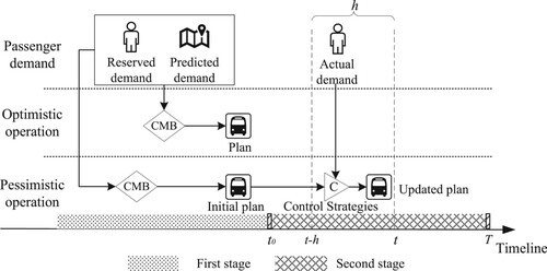
In the context of optimistic operation (see Section 4), the central system has the full information of $P_S$ and $P_F$ before operation (i.e.before timestamp $t_0$), and aims to minimise operating costs by jointly planning the CMB service. However, due to the reliance on demand predictions, in this context, there is no adaptation of the service to the real emerging demands during operation.

In the pessimistic operation scenario (see Section 5), the incoming demands may be significantly underestimated or overestimated, leading to greater resource wastage or unmet demands. Thus, a two-stage optimisation procedure is employed. The first stage formulates a deterministic and robust formulation, considering the penalty of unserved passengers, to produce initial plans with $P_S$ and $P_F$. The second stage involves periodic adjustment with control strategies, which can update the plans at each timestamp t within the operation period (from $t_0$ to T). Specifically, the central system evaluates predictive demands $P_F$ with actual needs $P_R$ collected during h to adjust plans at the end of h (i.e. timestamp t) accordingly.

Travel demand prediction. In this work, we utilise historical trips extracted from the bus SCD to generate predictions, following the methodology of R. Guo et al. (2019). Predictive processing includes three main activities: aggregation of ODs, feature extraction, and demand prediction. We extend the OD-based trip features by considering the time period, OD flow, day type, and demand size. Given the complexity and nature of the features, two state-of-the-art machine learning methods (namely LightGBM and AdaBoost), which have demonstrated their effectiveness in regression modelling, are selected via a preliminary set of experiments to deliver the accurate and less accurate predictions (Ke et al. 2017; Schapire 2013). It is worth noting that the proposed framework is independent of the specific tool used for generating predictions. For a more comprehensive description of our data processing and predictive methods, please refer to Section 6.2.

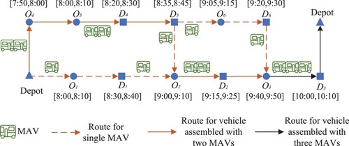
Modular feature. This paper explores the CMB system, which considers a set of fuel-based, homogeneous modules ($M=\{1,2,\dots ,|M|\}$) with a fixed capacity cap. One key feature of the system is that these modules can be assembled and disassembled into vehicles on roads, with different formations $w(w\in W)$ depending on the number of modules incorporated. This adaptability allows the CMB system to dynamically change its capacity to meet demands, making it highly flexible. Figure 2 shows an example of module assembling and disassembling operation based on the spatial and temporal travel requirements. The demand of $O_1\to D_1$ is 9 people, a 10-people module is dispatched with formation w = 1 to serve. After reaching $D_1$, this module is assembled with a module disassembled after visiting $O_4\to D_4$ and $O_5\to D_5$. This assembled vehicle with formation w = 2 continues serving 18 passengers of $O_2\to D_2$. Then, three dispatched modules are reassembled into a vehicle of formation w = 3, delivering 25 passengers from $O_3\to D_3$. It is noted that there is no passenger movement between modular units.

Figure 2. Proposed modular autonomous customised bus service.

Network representation. The CMB service design problem can be defined as a physical transportation network $(N,L)$, where the vertex set N consists of depot set O and demand vertices set S, L represents the set of directed links. Each directed link $(i,j)$ is associated with a time-dependent travel time $T{T}_{i,j,t}$ from vertex i to j departing from time t. The travel speed of each arc is a step function of the time, and the corresponding travel time function is a piecewise linear function (R. Guo et al. 2021). To integrate all decision-making into a unified optimisation framework, the network $(N,L)$ is extended to space-time-state network $G=(V,A)$, which combines travel time and load information. The space-time-state vertex $(i,t,k)$ indicates the module maintains the loading state k (i.e. the cumulative number of in-vehicle passengers) at vertex i at time t. A is the set of arcs. Each arc $(i,j,t,t^{\mathrm{\prime }},k,k^{\mathrm{\prime }})\in A$ is a space-time-state path from vertex $(i,t,k)$ to vertex $(j,t^{\mathrm{\prime }},k^{\mathrm{\prime }})$, signifying that the module travels through the physical arc $(i,j)$ during the time period ($t,t^{\mathrm{\prime }}$) with the loading state changing from k to $k^{\mathrm{\prime }}$. The time period $(t,t^{\mathrm{\prime }})$, considering the time-dependent travel time for $(i,j)$ and dwell time at j, can be treated as the service time needed for picking up or dropping off activities. The cumulative loading state k can capture the state transition for both pick-up and drop-off arcs. On a pick-up arc (with j as the pick-up vertex), passengers are picked up, and the loading state increases to $k^{\mathrm{\prime }}$ at j. On the drop-off arc (with j as the drop-off vertex), passengers are delivered and the loading state decreases to $k^{\mathrm{\prime }}$ at j. The state k should be $\ge 0$ and $\le cap$. The time horizon is uniformly divided into a series of 1-min intervals in the planning time horizon. In order to eliminate any infeasible arcs, the solution algorithm includes a set of constraints that take into account time windows and module capacity (Y. Wang et al. 2020).

Assumptions. The proposed CMB operational design problem is based on the following assumptions: (1) The reserved and predicted travel demands $P_S\cup P_F$ are known in advance, the actual demands $P_R$ of each h are known at the end of the interval, i.e. t. (2) All modules are fuel-based and homogeneous with the same capacity, each module ($m\in M$) starts and finishes the service between its earliest departure time $e^m$ and latest arrival time $l^m$ from the origin depot $o^m$ to destination depot $d^m$, with empty loading state $k_o$. (3) The travel time of each arc is time-variant and known, and a module departs from a vertex as early as possible. (4) Modules can be assembled and disassembled into different formations w with changeable capacity at any vertices during operation. (5) Passengers aggregated into one group $p(r\to s)$ are independent and can be served by different modules, but there is no passenger movement between modules. (6) When the pick-up arc $(i,j,t,t^{\mathrm{\prime }},k,k^{\mathrm{\prime }})\in A^r(p)$ is visited, the service time is within the time window $[e_r,l_r]$, the picked up passengers should $\le q_p$, when the drop-off arc $(i,j,t,t^{\mathrm{\prime }},k,k^{\mathrm{\prime }})\in A^s(p)$ is visited, the service time is within the time window $[e_s,l_s]$, the dropped off passenger should $\le q_p$. (7) Passenger loading state k cannot exceed the module capacity cap. The related notation is summarized in Table 1.

Table 1. Notation.

Symbol	Definition
Set and indices
N	Set of vertices, including depots and demand vertices
S	Set of pick-up and drop-off vertices
O	Set of depots
V	Set of space-time-state vertices
$P_S,P_F,P_R$	Set of reserved, predicted and actual passenger groups
$P_U$	Set of assigned but unserved passengers
M	Set of modules
T	Set of timestamps in the planning horizon
K	Set of cumulative passenger loading states of modules
$A_m$	Set of space-time-state arcs in module m's network
$A_m^r(p)$, $A_m^s(p)$	Set of pick-up and drop-off arcs of passenger group p in module m's network
i, j	Index of vertices, $i,j\in N$
$t,t^{\mathrm{\prime }}$	Index of time stamps, $t,t^{\mathrm{\prime }}\in T$
$k,k^{\mathrm{\prime }}$	Index of loading states, $k,k^{\mathrm{\prime }}\in K$
p	Index of passenger groups, $p\in P_S\cup P_F\cup P_R$
$(i,t,k),(j,t^{\mathrm{\prime }},k^{\mathrm{\prime }})$	Index of space-time-state vertices
$(i,j,t,t^{\mathrm{\prime }},k,k^{\mathrm{\prime }})$	Index of space-time-state arcs indicating that the module travels from vertex i at time t with loading state k to vertex j at time $t^{\mathrm{\prime }}$ with loading state $k^{\mathrm{\prime }}$
Parameters
$c_{i,j,t,t^{\mathrm{\prime }},k,k^{\mathrm{\prime }}}^w$	Travel cost on arc $(i,j,t,t^{\mathrm{\prime }},k,k^{\mathrm{\prime }})$ per module involved in formation w
$c_d^w$	Departure cost per module if it is involved in the vehicle with formation w
$c_p$	Penalty per unserved passenger of group p
$T{T}_{i,j,t}$	Arc travel time from vertex i to vertex j departing from time t
$o^m,d^m$	Origin and destination depots for module m
$e^m,l^m$	Earliest departure time and latest arrival time of m from $o^m$ to $d^m$
$k_o$	Empty loading state
λ	Minimum load requirement of each module
$q_p$	Passenger quantity of passenger group $p(p\in P_S\cup P_F)$
$q_p^{\mathrm{\prime }}$	Real passenger quantity of passenger group $p(p\in P_R)$
${\tilde{q}}_p$	Uncertain demand quantity of group p
${\hat{q}}_p$	Standard deviation demand of group p
$rat{e}_p$	Expected error rate of group p
${\delta }_p$	Deviation rate of group p, ${\delta }_p\in [-1,1]$
$[e_r,l_r],[e_s,l_s]$	Time window of pick-up vertex r and drop-off vertex s of passenger group p
η	Maximum vertices of changes allowed with respect to nominal plans $x_{i,j,t,t^{\mathrm{\prime }},k,k^{\mathrm{\prime }}}^{m\ast }$
Decision variables
$x_{i,j,t,t^{\mathrm{\prime }},k,k^{\mathrm{\prime }}}^{m,w}$	=1, if arc $(i,j,t,t^{\mathrm{\prime }},k,k^{\mathrm{\prime }})$ is passed through by module m incorporated to a vehicle of formation w; =0, otherwise
$y_p^m$	Number of passengers from group p served by module m
${ϵ}_p$	Number of unserved passengers of group p

4. Optimistic operation

This section introduces a mixed integer programming model to determine module movements, formations and P2M assignment in the time-dependent space-time-state network. Then, a Lagrangian relaxation approach is put forward to solve the model and find an optimal solution.

4.1. Mathematical model

Given the reserved and predictive demands ($P=P_S\cup P_F$), the CMB system aims to produce a solution encompassing routes, schedules, formations, and P2M assignments for assembled or disassembled modules. Based on the multi-dimension network, two decision variables are defined to minimise the operating cost:

• $x_{i,j,t,t^{\mathrm{\prime }},k,k^{\mathrm{\prime }}}^{m,w}\in \{0,1\}$, where $x_{i,j,t,t^{\mathrm{\prime }},k,k^{\mathrm{\prime }}}^{m,w}=1$ indicates that the arc $(i,j,t,t^{\mathrm{\prime }},k,k^{\mathrm{\prime }})$ is passed through by module m incorporated to a vehicle of formation w; otherwise, $x_{i,j,t,t^{\mathrm{\prime }},k,k^{\mathrm{\prime }}}^{m,w}=0$. This variable tracks the motion of each module while considering its formation. The formation w refers to whether m operates independently or in combination with other modules. This variable can understand and track the dynamic formation of modules as they move through the network.

• $y_p^m\ge 0$ denote the number of passengers from group p served by module m.

The CMB optimistic operation is presented as follows: (1) $\begin{array}{rl}min& L=TC+DC\\ \mathrm{s}.\mathrm{t}.& \text{Constraints }(2)-(13).\end{array}$(1) The objective (1(1) $\begin{array}{rl}min& L=TC+DC\\ \mathrm{s}.\mathrm{t}.& \text{Constraints }(2)-(13).\end{array}$(1) ) minimises the operating cost of a CMB system, taking into account the travelling cost TC of different module formations and departure cost DC presented as Equations (2(2) $\begin{array}{rl}TC& =\sum _{m\in M}\sum _{w\in W}\sum _{(i,j,t,t^{\mathrm{\prime }},k,k^{\mathrm{\prime }})\in A_m}{c}_{i,j,t,t^{\mathrm{\prime }},k,k^{\mathrm{\prime }}}^w{x}_{i,j,t,t^{\mathrm{\prime }},k,k^{\mathrm{\prime }}}^{m,w}\end{array}$(2) )–(3(3) $\begin{array}{rl}DC& =\sum _{m\in M}\sum _{w\in W}\sum _{(i,j,t,t^{\mathrm{\prime }},k,k^{\mathrm{\prime }})\in A_m:(i,t,k)\in \{(o^m,t,k_o)\}}{c}_d^w{x}_{i,j,t,t^{\mathrm{\prime }},k,k^{\mathrm{\prime }}}^{m,w}\end{array}$(3) ). Equation (2(2) $\begin{array}{rl}TC& =\sum _{m\in M}\sum _{w\in W}\sum _{(i,j,t,t^{\mathrm{\prime }},k,k^{\mathrm{\prime }})\in A_m}{c}_{i,j,t,t^{\mathrm{\prime }},k,k^{\mathrm{\prime }}}^w{x}_{i,j,t,t^{\mathrm{\prime }},k,k^{\mathrm{\prime }}}^{m,w}\end{array}$(2) ) shows that the travelling cost depends on the travelled distance of each module formation, which means TC is also related to the economy of scales. Equation (3(3) $\begin{array}{rl}DC& =\sum _{m\in M}\sum _{w\in W}\sum _{(i,j,t,t^{\mathrm{\prime }},k,k^{\mathrm{\prime }})\in A_m:(i,t,k)\in \{(o^m,t,k_o)\}}{c}_d^w{x}_{i,j,t,t^{\mathrm{\prime }},k,k^{\mathrm{\prime }}}^{m,w}\end{array}$(3) ) specifics that the departure cost is related to the formation in which modules are assembled at depots. It suggests that each module departs from its depot $o^m$ as an assembled vehicle with formation w at a designated time $t(t\in T)$ with an initial loading state of zero, i.e. $k_o=0$. (2) $\begin{array}{rl}TC& =\sum _{m\in M}\sum _{w\in W}\sum _{(i,j,t,t^{\mathrm{\prime }},k,k^{\mathrm{\prime }})\in A_m}{c}_{i,j,t,t^{\mathrm{\prime }},k,k^{\mathrm{\prime }}}^w{x}_{i,j,t,t^{\mathrm{\prime }},k,k^{\mathrm{\prime }}}^{m,w}\end{array}$(2) (3) $\begin{array}{rl}DC& =\sum _{m\in M}\sum _{w\in W}\sum _{(i,j,t,t^{\mathrm{\prime }},k,k^{\mathrm{\prime }})\in A_m:(i,t,k)\in \{(o^m,t,k_o)\}}{c}_d^w{x}_{i,j,t,t^{\mathrm{\prime }},k,k^{\mathrm{\prime }}}^{m,w}\end{array}$(3) Routing constraints. Constraints (4(4) $\begin{array}{rl}& \sum _{w\in W}\sum _{(i,j,t,t^{\mathrm{\prime }},k,k^{\mathrm{\prime }})\in A_m}{x}_{i,j,t,t^{\mathrm{\prime }},k,k^{\mathrm{\prime }}}^{m,w}=1,\mathrm{\forall }m\in M,i=o^m,t=e^m,k=k_o\end{array}$(4) )–(7(7) $\begin{array}{rl}& \sum _{m\in M}\sum _{w\in W}\sum _{(i,j,t,t^{\mathrm{\prime }},k,k^{\mathrm{\prime }})\in A_m^r(p)}{x}_{i,j,t,t^{\mathrm{\prime }},k,k^{\mathrm{\prime }}}^{m,w}\ge 1,\mathrm{\forall }p\in P_S\cup P_F\end{array}$(7) ) capture the movements of each module. Constraints (4(4) $\begin{array}{rl}& \sum _{w\in W}\sum _{(i,j,t,t^{\mathrm{\prime }},k,k^{\mathrm{\prime }})\in A_m}{x}_{i,j,t,t^{\mathrm{\prime }},k,k^{\mathrm{\prime }}}^{m,w}=1,\mathrm{\forall }m\in M,i=o^m,t=e^m,k=k_o\end{array}$(4) )–(6(6) $\begin{array}{rl}& \sum _{w\in W}\sum _{(j,t^{\mathrm{\prime }},k^{\mathrm{\prime }})\in V:(i,j,t,t^{\mathrm{\prime }},k,k^{\mathrm{\prime }})\in A_m}{x}_{i,j,t,t^{\mathrm{\prime }},k,k^{\mathrm{\prime }}}^{m,w}-\sum _{w\in W}\sum _{(j,t^{\mathrm{\prime }},k^{\mathrm{\prime }})\in V:(i,j,t,t^{\mathrm{\prime }},k,k^{\mathrm{\prime }})\in A_m}{x}_{j,i,t^{\mathrm{\prime }},t,k^{\mathrm{\prime }},k}^{m,w}=0,\\ & \mathrm{\forall }m\in M,(i,t,k)\notin \{(o^m,e^m,k_o),(d^m,l^m,k_o)\}\end{array}$(6) ) ensure each module departs from its origin depot and finally arrives at its destination depot, and make sure flow balance on every vertex in module m's space-time-state transportation network. Constraints (7(7) $\begin{array}{rl}& \sum _{m\in M}\sum _{w\in W}\sum _{(i,j,t,t^{\mathrm{\prime }},k,k^{\mathrm{\prime }})\in A_m^r(p)}{x}_{i,j,t,t^{\mathrm{\prime }},k,k^{\mathrm{\prime }}}^{m,w}\ge 1,\mathrm{\forall }p\in P_S\cup P_F\end{array}$(7) ) specify that any given demand arc can be visited by at least one module with any formation, ensuring that demand vertices can be served by either a disassembled single module or an assembled combination. (4) $\begin{array}{rl}& \sum _{w\in W}\sum _{(i,j,t,t^{\mathrm{\prime }},k,k^{\mathrm{\prime }})\in A_m}{x}_{i,j,t,t^{\mathrm{\prime }},k,k^{\mathrm{\prime }}}^{m,w}=1,\mathrm{\forall }m\in M,i=o^m,t=e^m,k=k_o\end{array}$(4) (5) $\begin{array}{rl}& \sum _{w\in W}\sum _{(i,j,t,t^{\mathrm{\prime }},k,k^{\mathrm{\prime }})\in A_m}{x}_{i,j,t,t^{\mathrm{\prime }},k,k^{\mathrm{\prime }}}^{m,w}=1,\mathrm{\forall }m\in M,j=d^m,t=l^m,k^{\mathrm{\prime }}=k_o\end{array}$(5) (6) $\begin{array}{rl}& \sum _{w\in W}\sum _{(j,t^{\mathrm{\prime }},k^{\mathrm{\prime }})\in V:(i,j,t,t^{\mathrm{\prime }},k,k^{\mathrm{\prime }})\in A_m}{x}_{i,j,t,t^{\mathrm{\prime }},k,k^{\mathrm{\prime }}}^{m,w}-\sum _{w\in W}\sum _{(j,t^{\mathrm{\prime }},k^{\mathrm{\prime }})\in V:(i,j,t,t^{\mathrm{\prime }},k,k^{\mathrm{\prime }})\in A_m}{x}_{j,i,t^{\mathrm{\prime }},t,k^{\mathrm{\prime }},k}^{m,w}=0,\\ & \mathrm{\forall }m\in M,(i,t,k)\notin \{(o^m,e^m,k_o),(d^m,l^m,k_o)\}\end{array}$(6) (7) $\begin{array}{rl}& \sum _{m\in M}\sum _{w\in W}\sum _{(i,j,t,t^{\mathrm{\prime }},k,k^{\mathrm{\prime }})\in A_m^r(p)}{x}_{i,j,t,t^{\mathrm{\prime }},k,k^{\mathrm{\prime }}}^{m,w}\ge 1,\mathrm{\forall }p\in P_S\cup P_F\end{array}$(7) Assignment constraints. Constraints (8(8) $\sum _{m\in M}{y}_p^m=q_p,\mathrm{\forall }p\in P_S\cup P_F$(8) ) make sure that each passenger group, whether composed of reserved or predicted passengers, has the flexibility to be assigned to multiple modules as required. (8) $\sum _{m\in M}{y}_p^m=q_p,\mathrm{\forall }p\in P_S\cup P_F$(8) Operation constraints. It enforces that the served passengers are greater than the minimum load factor to achieve long-term profits. In other words, modules can travel if they have a minimum number of passengers to serve, otherwise, it is economically unsustainable to run the service. (9) $\sum _{p\in P_S\cup P_F}{y}_p^m\ge \lambda ,\mathrm{\forall }m\in M$(9) Space-time-state constraints. They indicate that the module needs to visit both pick-up and drop-off arcs of paired OD (i.e. group p), and that the number of served passengers from p by this module is not greater than the total passengers of p. (10) $\begin{array}{rl}& y_p^m\le q_p\sum _{w\in W}\sum _{(i,j,t,t^{\mathrm{\prime }},k,k^{\mathrm{\prime }})\in A_m^r(p)}{x}_{i,j,t,t^{\mathrm{\prime }},k,k^{\mathrm{\prime }}}^{m,w},\mathrm{\forall }p\in P_S\cup P_F,m\in M\end{array}$(10) (11) $\begin{array}{rl}& y_p^m\le q_p\sum _{w\in W}\sum _{(i,j,t,t^{\mathrm{\prime }},k,k^{\mathrm{\prime }})\in A_m^s(p)}{x}_{i,j,t,t^{\mathrm{\prime }},k,k^{\mathrm{\prime }}}^{m,w},\mathrm{\forall }p\in P_S\cup P_F,m\in M\end{array}$(11) Module formation constraints. Constraints (12(12) $\begin{array}{rl}& \sum _{m\in M}\sum _{k\in K}\sum _{k^{\mathrm{\prime }}\in K}{x}_{i,j,t,t^{\mathrm{\prime }},k,k^{\mathrm{\prime }}}^{m,w}=w,\mathrm{\forall }(i,j,t,t^{\mathrm{\prime }},k,k^{\mathrm{\prime }})\in A,w\in W\end{array}$(12) ) enforce that the number of modules travelling from vertex i to vertex j during time period $(t,t^{\mathrm{\prime }})$ is equal to formation w. Constraints (13(13) $\begin{array}{rl}& \sum _{w\in W}{x}_{i,j,t,t^{\mathrm{\prime }},k,k^{\mathrm{\prime }}}^{m,w}\le 1,\mathrm{\forall }(i,j,t,t^{\mathrm{\prime }},k,k^{\mathrm{\prime }})\in A_m,m\in M\end{array}$(13) ) ensure that a module m travels through $(i,j,t,t^{\mathrm{\prime }},k,k^{\mathrm{\prime }})$ in any given formation w. (12) $\begin{array}{rl}& \sum _{m\in M}\sum _{k\in K}\sum _{k^{\mathrm{\prime }}\in K}{x}_{i,j,t,t^{\mathrm{\prime }},k,k^{\mathrm{\prime }}}^{m,w}=w,\mathrm{\forall }(i,j,t,t^{\mathrm{\prime }},k,k^{\mathrm{\prime }})\in A,w\in W\end{array}$(12) (13) $\begin{array}{rl}& \sum _{w\in W}{x}_{i,j,t,t^{\mathrm{\prime }},k,k^{\mathrm{\prime }}}^{m,w}\le 1,\mathrm{\forall }(i,j,t,t^{\mathrm{\prime }},k,k^{\mathrm{\prime }})\in A_m,m\in M\end{array}$(13) Note that the limitation is that passenger movements between modules are not considered explicitly, as we assume passengers will remain in the module they board. These simplifications allow us to focus on the flexible capacity afforded by the modularity and on the impact of predictions in the considered scenarios; investigations into extensions that address those assumptions are beyond the scope of this paper.

4.2. Solution approach

The proposed optimistic operational design problem is computationally challenging to be optimally solved, due to its NP-hardness. In this section, we introduce a Lagrangian heuristic algorithm to solve it. Lagrangian heuristic algorithm has already been used for large-scale optimisation problems, including a number of variants of vehicle routing problems (Tong et al. 2017).

4.2.1. Lagrangian relaxation

To solve the proposed mixed integer programming model, we first reformulate it by relaxing constraints (10(10) $\begin{array}{rl}& y_p^m\le q_p\sum _{w\in W}\sum _{(i,j,t,t^{\mathrm{\prime }},k,k^{\mathrm{\prime }})\in A_m^r(p)}{x}_{i,j,t,t^{\mathrm{\prime }},k,k^{\mathrm{\prime }}}^{m,w},\mathrm{\forall }p\in P_S\cup P_F,m\in M\end{array}$(10) )–(11(11) $\begin{array}{rl}& y_p^m\le q_p\sum _{w\in W}\sum _{(i,j,t,t^{\mathrm{\prime }},k,k^{\mathrm{\prime }})\in A_m^s(p)}{x}_{i,j,t,t^{\mathrm{\prime }},k,k^{\mathrm{\prime }}}^{m,w},\mathrm{\forall }p\in P_S\cup P_F,m\in M\end{array}$(11) ), which assemble variables $x_a^{m,w}$ (a is the abbreviation index of arc), and $y_p^m$. Two sets of multipliers ${\alpha }_p^m$ and ${\beta }_p^m$ are introduced to relax the corresponding constraints: (14) $\begin{array}{rl}minL(\alpha ,\beta )& =\sum _{m\in M}\sum _{w\in W}(\sum _{a\in A_m}{c}_a^w+\sum _{a\in A_m:(i,t,k)\in \{(o^m,t,k_o)\}}{c}_d^w)x_a^{m,w}\\ & +\sum _{p\in P_S\cup P_F}\sum _{m\in M}{\alpha }_p^m(y_p^m-q_p\sum _{w\in W}\sum _{a\in A_m^r(p)}{x}_a^{m,w})\\ & +\sum _{p\in P_S\cup P_F}\sum _{m\in M}{\beta }_p^m(y_p^m-q_p\sum _{w\in W}\sum _{a\in A_m^s(p)}{x}_a^{m,w})\\ \mathrm{s}.\mathrm{t}.& \text{Constraints }(4)-(9),(12)-(13).\end{array}$(14) The new Lagrangian relaxation problem can be decomposed into two sub-problems, namely module routing and formation problem (MRFP) and P2M assignment problem (PAP):

Subproblem 1: MRFP (SP1(α,β)): (15) $\begin{array}{rl}minSP1(\alpha ,\beta )& =\sum _{m\in M}\sum _{w\in W}\sum _{a\in A_m}(c_a^w+c_d^w)x_a^{m,w}\\ & -\sum _{p\in P_S\cup P_F}\sum _{m\in M}\sum _{w\in W}{q}_p({\alpha }_p^m\sum _{a\in A_m^r(p)}{x}_a^{m,w}+{\beta }_p^m\sum _{a\in A_m^s(p)}{x}_a^{m,w})\\ \mathrm{s}.\mathrm{t}.& \text{Constraints }(4)-(7),(12)-(13).\end{array}$(15) Subproblem 2: PAP (SP2(α,β)): (16) $\begin{array}{rl}min& SP2(\alpha ,\beta )=\sum _{p\in P_S\cup P_F}\sum _{m\in M}({\alpha }_p^m+{\beta }_p^m)y_p^m\\ \mathrm{s}.\mathrm{t}.& \text{Constraints }(8)-(9).\end{array}$(16)

4.2.2. Feasible solution generation

The Lagrangian relaxation can calculate the lower bounds of the model. However, as the space-time-state constraints are relaxed, the optimal solution of lower bounds may only satisfy P2M assignment restrictions. Thus, a feasible solution using the optimal routes of the relaxation problems is generated to obtain the upper-bound solution.

Specifically, if the developed relaxed plan is a feasible solution to the primal problem, this solution is available to update the upper bound directly; otherwise, the modification procedure will be triggered when module routes do not satisfy the passengers' travel requirements. We use the routing and formation solution of $SP1$ to check whether the supplied CMB service fulfils each travel request. For each request, passengers are assigned across the modules travelling through the corresponding arcs, based on the remaining module capacity and unassigned passengers. If the provided capacities are sufficient, passengers are inserted into the current routing plan; otherwise, the unassigned passengers are sent to a request pool. Then, new modules are activated to cater to these demands. The updating $SP1$ solution is used to compute the upper bounds. The details for generating a feasible solution are shown in Algorithm 1.

4.2.3. Sub-gradient method

Generally, the standard sub-gradient algorithm is adopted to iteratively update the Lagrangian multipliers that are given in Section 4.2.1, when calculating the upper and lower bounds of the relaxation problem (Pu and Zhan 2021). The initial multipliers are set to 0. Then the multipliers ${\mathit{\alpha }}^{n+1}$ and ${\mathit{\beta }}^{n+1}$ in iteration n + 1 can be updated based on the sub-gradient directions of relaxed constraints, an example is given with ${\mathit{\alpha }}^{n+1}$: (17) ${\mathit{\alpha }}^{n+1}=max\{0,{\mathit{\alpha }}^n+{\xi }^n(y_p^{m,n}-q_p\sum _{w\in W}\sum _{a\in A_m^r(p)}{x}_a^{m,w,n})\}$(17) where $x_a^{m,w,n}$, $y_p^{m,n}$ are the solutions of the sub-problems at iteration n, the step size ${\xi }^n$ is defined in Equation (18(18) ${\xi }^n=\frac{{\theta }^n(UB(n)-LB(n))}{{\Vert ▽({\mathit{\alpha }}^n)\Vert }^2}$(18) ), the step size ${\eta }^n$ used for ${\mathit{\beta }}^{n+1}$ is defined with similar way. (18) ${\xi }^n=\frac{{\theta }^n(UB(n)-LB(n))}{{\Vert ▽({\mathit{\alpha }}^n)\Vert }^2}$(18) where $UB(n)$ and $LB(n)$ are the best upper and lower bounds in iteration n. The range of ${\theta }^n$ is in the interval of [0, 1] to accelerate the calculations.

The details of the proposed Lagrangian heuristic algorithm are as follows.

Step 1: (Initialization). Initialize the Lagrangian multiplier ${\mathit{\alpha }}^{\mathit{n}}$ and ${\mathit{\beta }}^{\mathit{n}}$, set the iteration index n = 0.

Step 2: (Lower bound generation). Solve the subproblems $SP1(\alpha ,\beta )$ and $SP2(\alpha ,\beta )$ with CPLEX, and compute the $LB=max\{LB,SP1+SP2\}$ with ${\mathit{x}}^{\mathit{n}}$ and ${\mathit{y}}^{\mathit{n}}$.

Step 3: (Upper bound generation). Determine the substituting ${\mathit{x}}^{\mathit{n}}$, the ${\mathit{y}}^{\mathit{n}}$ with Algorithm 1, and compute the $UB=min\{UB,SP1+SP2\}$.

Step 4: (Update Lagrangian multipliers). Update the multipliers by the sub-gradient method.

Step 5: (Termination condition). Terminate if the relative gap between LB and UP is below the threshold γ.

5. Pessimistic operation

This section is devoted to introducing the two-stage optimisation procedure used in the case of pessimistic operation. For the sake of this investigation, we assume that it is possible to estimate the expected error of a predictive model, for instance, by comparing predictions with available historical data.

Figure 1 shows that the initial plan solutions are generated in the first stage. However, given the potential of overestimation or underestimation of demands due to the less accurate predictions, it is likely that the CMB services will be overutilized or underserved, which can lead to significant unserved passengers or no-show passenger services. Thus, a deterministic optimisation model offering partial services (i.e.conservative plans) is proposed to minimise the penalty caused by unserved passengers on board. In addition, a nominal-plan-based robust model is introduced to capture the risk-averse level of the system in an uncertain demand environment. We first report two formulations are presented in Sections 5.1 and 5.2; Both formulations are tackled using the Lagrangian relaxation, which is subsequently presented. Finally, the second stage with control strategies is given in Section 5.3 to update the service to the actual requests at each timestamp.

5.1. First stage-deterministic optimization model with penalty

This section formulates the problem as a deterministic model with a penalty, which can reduce the waste of resources by ignoring some predicted passengers. The detailed formulation and solution approach are given below.

5.1.1. Mathematical model

To recognise the quality of predictions, we define the expected error rate $rat{e}_p$ of each group p. This parameter can be calculated using the real (or expected due to historical data) demand $q_p^{\mathrm{\prime }}$ and predictive data $q_p$. Then, we categorise the predicted data into three classes based on the error rate: (i) underestimated groups, i.e. $rat{e}_p\in [-50\mathrm{\%},0\mathrm{\%}]$; (ii) overestimated groups, i.e. $rat{e}_p\in [0\mathrm{\%},50\mathrm{\%}]$ and (iii) overlooked groups ($rat{e}_p<-50\mathrm{\%}$ or $>50\mathrm{\%}$). (19) $rat{e}_p=(q_p-q_p^{\mathrm{\prime }})/q_p^{\mathrm{\prime }}$(19) To alleviate the supply-demand imbalance potentially caused by predictions, we introduce a deterministic model that considers the trade-off between operating cost and penalty caused by unserved passengers, on top of the model proposed in Section 4.1, as follows: (20) $\begin{array}{rl}min& L=TC+DC+PC\\ \mathrm{s}.\mathrm{t}.& \text{Constraints }(2)-(7),(9)-(13),(21)-(23).\end{array}$(20) The objective (20(20) $\begin{array}{rl}min& L=TC+DC+PC\\ \mathrm{s}.\mathrm{t}.& \text{Constraints }(2)-(7),(9)-(13),(21)-(23).\end{array}$(20) ) aims to minimise the operating costs (TC and DC) and the penalty arising from unserved passengers. Equation (21(21) $PC=\sum _{p\in P_F}{c}_p(q_p-\sum _{m\in M}{y}_p^m)$(21) ) indicates that if passengers from predicted groups are not picked up, a penalty is imposed on the system. (21) $PC=\sum _{p\in P_F}{c}_p(q_p-\sum _{m\in M}{y}_p^m)$(21) Assignment constraints. Constraints (22(22) $\begin{array}{rl}& \sum _{m\in M}{y}_p^m=q_p,\mathrm{\forall }p\in P_S\end{array}$(22) ) ensure that all passengers from reserved groups are served, reflecting our commitment to fulfilling pre-determined reservations. Constraints (23(23) $\begin{array}{rl}& \sum _{m\in M}{y}_p^m\{\begin{array}{l}=q_p,\mathrm{if}rat{e}_p\in [-50\mathrm{\%},0\mathrm{\%}],\\ \le q_p,\mathrm{if}rat{e}_p\in [0\mathrm{\%},50\mathrm{\%}],\\ =0,\mathrm{if}rat{e}_p<-50\mathrm{\%}\mathrm{or}>50\mathrm{\%},\end{array}\mathrm{\forall }p\in P_F\end{array}$(23) ) suggest that the assignment of passengers within predicted groups is influenced by the calculated expected error rate $rat{e}_p$, which indicates that the system adjusts its service level based on predictive accuracy: providing full, partial and no services for underestimated, overestimated and overlooked requests. (22) $\begin{array}{rl}& \sum _{m\in M}{y}_p^m=q_p,\mathrm{\forall }p\in P_S\end{array}$(22) (23) $\begin{array}{rl}& \sum _{m\in M}{y}_p^m\{\begin{array}{l}=q_p,\mathrm{if}rat{e}_p\in [-50\mathrm{\%},0\mathrm{\%}],\\ \le q_p,\mathrm{if}rat{e}_p\in [0\mathrm{\%},50\mathrm{\%}],\\ =0,\mathrm{if}rat{e}_p<-50\mathrm{\%}\mathrm{or}>50\mathrm{\%},\end{array}\mathrm{\forall }p\in P_F\end{array}$(23)

5.1.2. Lagrangian relaxation

By relaxing constraints (10(10) $\begin{array}{rl}& y_p^m\le q_p\sum _{w\in W}\sum _{(i,j,t,t^{\mathrm{\prime }},k,k^{\mathrm{\prime }})\in A_m^r(p)}{x}_{i,j,t,t^{\mathrm{\prime }},k,k^{\mathrm{\prime }}}^{m,w},\mathrm{\forall }p\in P_S\cup P_F,m\in M\end{array}$(10) ) and (11(11) $\begin{array}{rl}& y_p^m\le q_p\sum _{w\in W}\sum _{(i,j,t,t^{\mathrm{\prime }},k,k^{\mathrm{\prime }})\in A_m^s(p)}{x}_{i,j,t,t^{\mathrm{\prime }},k,k^{\mathrm{\prime }}}^{m,w},\mathrm{\forall }p\in P_S\cup P_F,m\in M\end{array}$(11) ), the new Lagrangian relaxation problem of the deterministic model can be decomposed into two sub-problems, where the module routing and formation problem (SP1) is similar to those presented in Section 4.2.1. The relaxed problem SP2 is defined as the P2M assignment problem with the penalty (PAP-P):

Subproblem 2: PAP-P (SP2(α,β)): (24) $\begin{array}{rl}min& SP2(\alpha ,\beta )=\sum _{p\in P_S\cup P_F}\sum _{m\in M}({\lambda }_p^m+{\beta }_p^m)y_p^m+\sum _{p\in P_F}{c}_p(q_p-\sum _{m\in M}{y}_p^m)\\ \mathrm{s}.\mathrm{t}.& \text{Constraints }(9),(22)-(23).\end{array}$(24) The decomposed problems can be solved by the Lagrangian heuristic algorithm introduced in Section 4.2.

5.2. First stage-robust optimization model

Let us point out that the introduced pessimistic design problem can also be considered an operational problem under uncertain demand (Dou, Meng, and Liu 2021). For this reason, we can also take inspiration from approaches implemented for treating the focussed problem with an uncertainty set. The robust optimisation approach has been chosen due to its excellent performance in similar scenarios (X. Guo, Caros, and Zhao 2021). Integrating robustness into the module routing, scheduling and formation design is one way to protect solutions against uncertain conditions (Santos et al. 2020).

5.2.1. Mathematical model

The robust optimisation approach presented here follows the box uncertainty set introduced by Bertsimas, Pachamanova, and Sim (2004) to characterise demand uncertainty. The demand concerning group $p(p\in P_F)$ is represented by ${\tilde{q}}_p$; it is treated as uncertain demand that can change to any value within the defined range. We bound the uncertain demand ${\tilde{q}}_p\in [q_p-{\hat{q}}_p,q_p+{\hat{q}}_p]$, where $q_p$ denote the nominal demands obtained from the predicted data of the group p, and ${\hat{q}}_p$ denote the standard deviation demand representing the difference between the predicted data and the actual requests (can be obtained based on historical data). $q_p$ can be viewed as the mean of ${\tilde{q}}_p$. The deviation rate ${\delta }_p\in [-1,1]$ of group p is defined as: (25) ${\delta }_p=({\tilde{q}}_p-q_p)/q_p$(25) As the estimated data is classified into overestimation ($rat{e}_p>0$) and underestimation ($rat{e}_p\le 0$) demands, the uncertain demands ${\tilde{q}}_p$ for overestimation have a falling state ${\tilde{q}}_p\in [q_p-{\hat{q}}_p,q_p]$, while they have a rising state ${\tilde{q}}_p\in [q_p,q_p+{\hat{q}}_p]$ for underestimation case.

The proposed robust formulation increases the robustness of the routing and scheduling decisions (Cacchiani, Qi, and Yang 2020), which derives the new solutions based on the nominal plans generated for reserved demands and the nominal demands of predictive data. To maintain the feasibility of the robust model, we consider the slack decision variable and nominal plans. Besides, a limit is imposed to restrict changes in the nominal plans, as follows:

• ${ϵ}_p\ge 0$ denote the number of unserved passengers of a group p.

• $x_{i,j,t,t^{\mathrm{\prime }},k,k^{\mathrm{\prime }}}^{m,w\ast }\in \{0,1\}$ denote the nominal plans.

• η is the maximum vertices of changes allowed with respect to $x_{i,j,t,t^{\mathrm{\prime }},k,k^{\mathrm{\prime }}}^{m,w\ast }$.

(26) $\sum _{(i,j,t,t^{\mathrm{\prime }},k,k^{\mathrm{\prime }})\in A_m}|x_{i,j,t,t^{\mathrm{\prime }},k,k^{\mathrm{\prime }}}^{m,w}-x_{i,j,t,t^{\mathrm{\prime }},k,k^{\mathrm{\prime }}}^{m,w\ast }|\le \eta ,\mathrm{\forall }m\in M,w\in W$(26) Based on the notations above, the robust formulation based on the nominal plan is formulated as: (27) $\begin{array}{rl}min& L=TC+DC+PC\\ \mathrm{s}.\mathrm{t}.& \text{Constraints }(2)-(7),(9)-(13),(26),(28)-(30).\end{array}$(27) The objective (28(28) $PC=\sum _{p\in P_F}{c}_p{ϵ}_p$(28) ) aims to minimise the operating cost and penalty incurred by unserved passengers. (28) $PC=\sum _{p\in P_F}{c}_p{ϵ}_p$(28) Assignment constraints. Constraints (29(29) $\begin{array}{rl}& \sum _{m\in M}{y}_p^m=q_p,\mathrm{\forall }p\in P_S\end{array}$(29) ) state the assignment of reserved demands. Constraints (30(30) $\begin{array}{rl}& \sum _{m\in M}{y}_p^m+{ϵ}_p={\tilde{q}}_p,\mathrm{\forall }p\in P_F,m\in M\end{array}$(30) ) insert the slack variable ${ϵ}_p$, encoding that the number of served and unserved passengers are equal to the uncertainty demand. (29) $\begin{array}{rl}& \sum _{m\in M}{y}_p^m=q_p,\mathrm{\forall }p\in P_S\end{array}$(29) (30) $\begin{array}{rl}& \sum _{m\in M}{y}_p^m+{ϵ}_p={\tilde{q}}_p,\mathrm{\forall }p\in P_F,m\in M\end{array}$(30) The slack decision variable ${ϵ}_p$ can be represented by the passenger assignment variable $y_p^m$ according to constraints (30(30) $\begin{array}{rl}& \sum _{m\in M}{y}_p^m+{ϵ}_p={\tilde{q}}_p,\mathrm{\forall }p\in P_F,m\in M\end{array}$(30) ), and Equation (28(28) $PC=\sum _{p\in P_F}{c}_p{ϵ}_p$(28) ) can be represented as Equation (32(32) $\begin{array}{rl}PC& =\sum _{p\in P_F}{c}_p({\tilde{q}}_p-\sum _{m\in M}{y}_p^m)\end{array}$(32) ): (31) $\begin{array}{rl}{ϵ}_p& ={\tilde{q}}_p-\sum _{m\in M}{y}_p^m,\mathrm{\forall }p\in P_F,m\in M\end{array}$(31) (32) $\begin{array}{rl}PC& =\sum _{p\in P_F}{c}_p({\tilde{q}}_p-\sum _{m\in M}{y}_p^m)\end{array}$(32)

5.2.2. Lagrangian relaxation

Similar to Section 4.2.1, the introduced robust model can be relaxed into two subproblems. The nominal-plan-based module routing and formation problem (NMRFP), and the uncertain P2M assignment problem (UPAP), are presented below:

Subproblem 1: NMRFP (SP1(α, β)): (33) $\begin{array}{rl}min& SP1(\alpha ,\beta )=\sum _{m\in M}\sum _{w\in W}\sum _{a\in A_m}(c_a^w+c_d^w)x_a^{m,w}\\ & -\sum _{p\in P_S\cup P_F}\sum _{m\in M}\sum _{w\in W}{q}_p({\alpha }_p^m\sum _{a\in A_m^r(p)}{x}_a^{m,w}+{\beta }_p^m\sum _{a\in A_m^s(p)}{x}_a^{m,w})\\ \mathrm{s}.\mathrm{t}.& \text{Constraints }(4)-(7),(12)-(13),(26).\end{array}$(33) Subproblem 2: UPAP (SP2(α,β)): (34) $\begin{array}{rl}min& SP2(\alpha ,\beta )=\sum _{p\in P_S\cup P_F}\sum _{m\in M}({\lambda }_p^m+{\beta }_p^m)y_p^m+\sum _{p\in P_F}{c}_p({\tilde{q}}_p-\sum _{m\in M}{y}_p^m)\\ \mathrm{s}.\mathrm{t}.& \text{Constraints }(9),(29)-(30).\end{array}$(34) The decomposed problems can then be solved by the proposed Lagrangian heuristic algorithm.

5.3. Second stage-control strategies

In this section, we focus on the second stage of the proposed pessimistic operational design, which is in charge of adjusting the plan generated by either of the proposed approaches, to the actual demands. Note that plans are adjusted at each timestamp t within the planning horizon, where actual demands are known for every time period h corresponding to the predictive time window. For the sake of readability, Figure 3 shows the four scenarios corresponding to cases where adjustments regarding the original plans are needed.

Figure 3. Adjustment scenarios with undersupply and oversupply.

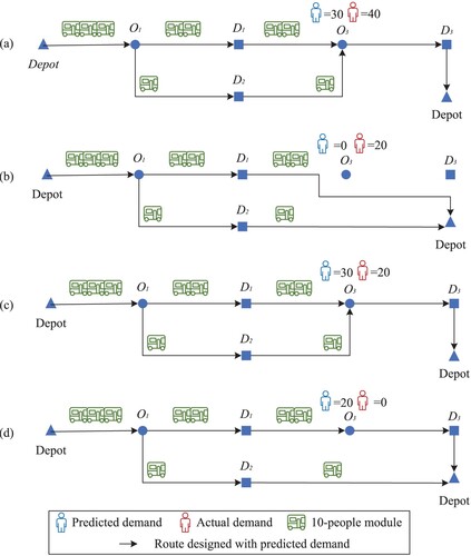
Figure 3(a,b) illustrates the undersupply cases when the actual passengers of group p are greater than the predicted demand of p. In Figure 3(a), the actual demand of passenger group $p(O_3\to D_3)$ contains 40 passengers that is higher than the predicted 30 people. If no adjustment is put in place, this will result in unserved demands of 10 passengers, due to the limited capacity provided by the vehicle assembled with three 10-people modules. Figure 3(b) shows an example where the provided predictions do not contain group $p(O_3\to D_3)$, and the initial plans are not allowed to serve this request, even though there are 20 people appearing for this OD. Figures 3(c,d) are instead cases of oversupply. The excess capacity of 10 people wastes capacity as the actual demand is less than the predicted one in Figure 3(c). Finally, Figure 3(d) represents a no-show passenger scenario.

Here, we design two strategies for undersupply or oversupply situations. Undersupply is addressed by activating new modules or inserting additional demand into existing services. Oversupply drives the system to skip the planned route and reduce the module capacity. The corresponding two strategies are presented as follows.

5.3.1. Passenger-reassignment control

Passenger reassignment jointly considers the unserved passengers in Figure 3(a,b) due to unexpected demands, as well as the en-route and idle modules in the adjustment procedure, and allows scheduling. When $q_p<q_p^{\mathrm{\prime }}$ or $q_p=0,q_p^{\mathrm{\prime }}>0$, and there is available capacity in the running modules, then assign extra passengers into the initial plans and update P2M assignment: (35) $\sum _{m\in M}{y}_p^m=q_p^{\mathrm{\prime }},\mathrm{\forall }p\in P_R$(35) Otherwise, the unserved and newly emerging passengers are served by activating new modules, as shown in the formulation of Section 4.1.

5.3.2. Skip-stop and module-disassemble control

This strategy considers en-route modules, and allows to change route and schedule plans. When the predicted data is higher than the actual requests, as shown in Figure 3(c), this strategy is triggered to reduce the supplied capacity by disassembling modules from the current formation. To be specific, the supplied modules are re-determined according to the capacity required by including passengers who are assigned but not yet served of $p(r\to s)(p\in P_U)$, and actual requests $q_p^{\mathrm{\prime }}$ of p. The module is removed from the plans (generated at timestamp t−h, t−h is the last adjustment timestamp) at timestamp t. $\breve{y_p^m}$ and $\breve{w}$ denote the P2M assignment, module formation and scheduling at t−h. (36) $\begin{array}{rl}w\cdot cap& =\sum _{p\in P_U\mathrm{\setminus }\{p\}}\sum _{m\in M}(\breve{y_p^m}+q_p^{\mathrm{\prime }}),\mathrm{\forall }w\in W\end{array}$(36) (37) $\begin{array}{rl}\breve{w}-w& =\sum _{m\in M}\sum _{a\in A_m^r(p)}{x}_a^{m,\breve{w}}-\sum _{m\in M}\sum _{a\in A_m^r(p)}{x}_a^{m,w},\mathrm{\forall }p\in P_U,\breve{w},w\in W\end{array}$(37) Equation (36(36) $\begin{array}{rl}w\cdot cap& =\sum _{p\in P_U\mathrm{\setminus }\{p\}}\sum _{m\in M}(\breve{y_p^m}+q_p^{\mathrm{\prime }}),\mathrm{\forall }w\in W\end{array}$(36) ) re-determines the module supply at t. Equation (37(37) $\begin{array}{rl}\breve{w}-w& =\sum _{m\in M}\sum _{a\in A_m^r(p)}{x}_a^{m,\breve{w}}-\sum _{m\in M}\sum _{a\in A_m^r(p)}{x}_a^{m,w},\mathrm{\forall }p\in P_U,\breve{w},w\in W\end{array}$(37) ) implies that the module formation and routing are changed from t−h to t, with the module disassembling.

When $q_p^{\mathrm{\prime }}=0$ as shown in Figure 3(d), the skip-stop tactic is triggered to prevent accessing origin r and destination s of p. The vertices are removed from the plans as shown in Equation (38(38) $\sum _{m\in M}\sum _{w\in W}\sum _{a\in A_m^r(p)}{x}_a^{m,w}+\sum _{m\in M}\sum _{w\in W}\sum _{a\in A_m^s(p)}{x}_a^{m,w}=0$(38) ), and the module disassembling is triggered with Equations (36(36) $\begin{array}{rl}w\cdot cap& =\sum _{p\in P_U\mathrm{\setminus }\{p\}}\sum _{m\in M}(\breve{y_p^m}+q_p^{\mathrm{\prime }}),\mathrm{\forall }w\in W\end{array}$(36) )–(37(37) $\begin{array}{rl}\breve{w}-w& =\sum _{m\in M}\sum _{a\in A_m^r(p)}{x}_a^{m,\breve{w}}-\sum _{m\in M}\sum _{a\in A_m^r(p)}{x}_a^{m,w},\mathrm{\forall }p\in P_U,\breve{w},w\in W\end{array}$(37) ). (38) $\sum _{m\in M}\sum _{w\in W}\sum _{a\in A_m^r(p)}{x}_a^{m,w}+\sum _{m\in M}\sum _{w\in W}\sum _{a\in A_m^s(p)}{x}_a^{m,w}=0$(38)

6. Experimental analysis

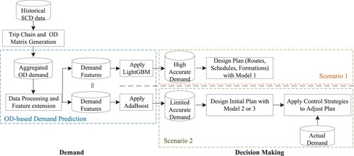
This experimental analysis aims to demonstrate the usefulness of the framework exploited for CMB systems, and to assess the strengths and weaknesses of the proposed approaches, using a large-scale network from the city of Beijing, China. Figure 4 provides the flowchart of the experimental methodology. Two machine learning techniques (LightGBM and AdaBoost) are employed to yield two distinct prediction scenarios. When dealing with highly accurate predictions, the optimistic operation is activated, where Model 1 (detailed in Section 4.1) is employed to tailor services. The operation mode turns to a pessimistic one when tackling predictions of limited accuracy: deterministic or robust model (Model 2 and Model 3) is deployed to outline initial service plans; control strategies are triggered to dynamically update services in response to discrepancies. All models can be solved by the solution approach proposed in Section 4.2.

Figure 4. Flowchart illustrating the process of the experimental methodology, from data collection to implementation, highlighting the two distinct predictions and their corresponding optimisation scenarios.

The experimental settings are presented in Section 6.1. Section 6.2 presents the OD-based demand prediction and evaluates the ability of predictive models. Then, in Section 6.3, we compare the performance of optimistic and pessimistic operations. Finally, Sections 6.4 and 6.5 analyse the impact of module capacity and time-dependent travel time on CMB services. Owing to the lack of time-related travel times for 2019 aligned with the demand data year, we assume the constant travel speed in Sections 6.3 and 6.4, while time dependency effects are explored in Section 6.5 leveraging time-varying travel time data from 2015. This relative analysis can gain valuable insights, despite potential discrepancies in the data. We conduct our experiments with Python 3.7 and CPLEX 12.8 on a computer with a 3.4 GHz CPU and 16 GB of RAM.

6.1. Experimental settings

The experiments are carried out with the bus smartcard data and the road network of Beijing, China. The SCD contains approximately 12 million travel records daily from November 2018 to February 2019. Each travel record is associated with attributes including card IDs, route numbers, boarding and alighting events. Besides the SCD, we also use the route and station data of the conventional bus system in Beijing, which contains the longitude and latitude position of each station.

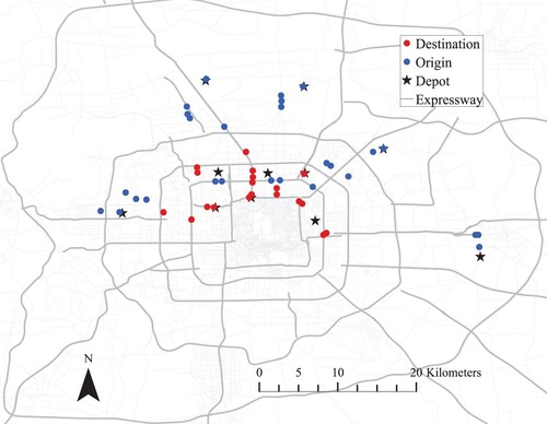
Data generation. We focus on the commuter trips expected to be the main potential demands of CB services (Qiu et al. 2018). We consider the working days between 3rd December 2018 to 18th January 2019 for training, and the days from 21st to 25th January 2019 for testing, which avoids the restrictions or influences of COVID-19 pandemic and the Chinese Lunar New Year. To extract the outflow from residential areas and the inflow to working places during morning peak (7:00–9:00 AM), we select records of trips from typical residential communities to business districts, and follow the methodology introduced in R. Guo et al. (2019) to identify the aggregated OD demands, as shown in Figure 4. Figure 5 gives the distribution of the extracted stations for commuting trips regarding the Beijing metropolitan area.

Figure 5. Distribution of OD for the extracted travel demands in Beijing, China, was initially applied to in R. Guo et al. (2021).

Parameter setting. We assume a homogeneous fleet of 28 modules with a capacity of 15 people. Considering the maximal physical length for safe operation on urban roads with limited width and turns, modules of about 5.5 meters can be assembled or disassembled into three formations ($W=\{1,2,3\}$), corresponding to the departure cost per module of 550, 450, and 370 (unit: ¥), based on data from minibuses and X. Liu, Qu, and Ma (2021) and R. Guo et al. (2023). The travelling cost per distance per module is set as 20, 17.97, 16.18 (unit: ¥) for three formations, as the travelling cost per distance is not a linear function of formations. The constant travel speed is 20km/h. The minimum load requirement per module is 10 people. The travel cost is ¥20 for space-time-state arc, the service time for each vertex is 1 minute. The penalty incurred per unserved passenger is ¥10, and the maximum vertices of changes η is 2. The gap of Lagrangian relaxation heuristic algorithm is set as <3%, and the maximum total number of iterations is 50.

Instance generation. To evaluate the performance of CMB under varying passenger distribution, three distinct instances have been created: R (random), C (clustered), and RC (mixed), each signifying a different type of passenger distribution, that can refer to R. Guo et al. (2023). Every instance contains 50 groups totalling around 300 passengers. Among these groups, 10 are dedicated to reserved demands, while the remaining 40 cater to incoming demands.

6.2. OD-based demand prediction

This section describes the prediction procedure of emerging requests, where the data processing for feature extension, predictive models, and performance evaluation are discussed herein.

6.2.1. Data processing

The prediction problem at hand is dealt with as a regression problem, where the goal is to predict the number of passengers that will require to use the CMB services between each possible OD in a considered time window. To better use the demand features for prediction, it is necessary to understand the spatial-temporal dynamics of OD flow at a given period. Table 2 shows the set of features considered, including the original features obtained from the raw OD demands, and the features derived to support the work of the predictive models.

Table 2. Original and Extracted Features for the considered dataset, with the corresponding type and format.

Original features	Extracted features	Type	Format
Date	Date	Datetime	e.g. 1/1/2018
	Week Day	Categorical	Mon, Tues, Wed, Thurs, Fri
	DayType	Categorical	Weekday vs Mon vs Fri
Timestamp	Time period	Categorical	e.g. 700–730 as Timestamp_1
Origin	OriDes	Categorical	1018–1020 as OD_1,
Destination			1020–1018 as OD_2
Demand	Size	Integer	Numeric value
	Presence	Boolean	Yes or No

The time period for which the demand has been assessed is divided into 5 intervals of 7:00–7:30 am, 7:30–7:45 am, 7:45–8:00 am, 8:00–8:15 am, 8:15–8:30 am, where the first corresponds to the reserved demands (10 groups), the remaining are the forecast time windows for incoming demands (40 groups). Each interval contains 10 passenger groups. From the original date feature, two variables have been derived: the day of the week, and the type of the day (Monday, Friday, other weekdays).

Correlation analysis has been applied to all the original and derived variables and no correlation is found between the variables, thus supporting the usage of all the variables for predictive modelling.

6.2.2. Predictive models

Given the types and characteristics of the features, and considering the approaches at the state-of-the-art of regression, this work focuses on the so-called ensemble learning, where multiple learning methods are used together to improve the overall predictive performance. Learning methods can be combined in parallel (bagging) or sequence (boosting).

After running a set of preliminary experiments with an extensive range of approaches, two ensemble methods, LightGBM and AdaBoost, are selected for optimistic and pessimistic operations, respectively. Adaboost (Adaptive Boost) is a boosting ensemble method that adds many decision ‘stumps’ (decision trees with only one split) sequentially to generate a strong learner. Different from AdaBoost, LightGBM can use both bagging or boosting (Ke et al. 2017). It also permits the model to choose between different gradient boosting methods: GBDT, DART and GOSS to best suit the problem statement (Barros, Cerqueira, and Soares 2021).

To boost the performance of these models, we optimise their hyper-parameters using Grid Search Cross Validation. Parameters considered for optimisation for Adaboost include the number of estimators and their type, and the learning rate. Similarly, for LightGBM, the parameters chosen for tuning are boosting type (GBDT, DART, GOSS), L1 and L2 regularisation along with learning rate, maximum depth of sub-trees, minimum child samples on a sub-tree, number of estimators, and number of leaves in a sub-tree.

6.2.3. Prediction evaluation

To assess the achieved performance, we used the standard metrics of mean absolute error (MAE), mean squared error (MSE), and root mean squared error (RMSE). MAE evaluates the average of the differences between the actual values and the predictions of the observations. MSE is the average of the square of these differences, and RMSE is the square root of the average of the square of the differences.

The performance of the models for each considered testing day is shown in Table 3. Further, the table provides the R${}^2$ results, the explained variance, and the maximum prediction error on an OD demand. R${}^2$ is the well-known coefficient of determination. The explained variance is a measure of the proportion of the variability of the predictions concerning the actual data.

Table 3. For the considered predictive models, the performance achieved on each testing day in terms of RMSE, MSE, MAE, $R^2$, explained variance and maximum error.

Date	model	RMSE	MSE	MAE	R${}^2$	ex_var	max_e
21st	AdaBoost	4.545	20.66	13.795	0.2798	0.453	12
	LightGBM	1.467	2.15	1.009	0.9250	0.924	5
22nd	AdaBoost	4.387	19.25	13.561	0.2766	0.458	11
	LightGBM	1.388	1.93	0.968	0.9276	0.927	6
23rd	AdaBoost	5.235	27.41	14.286	0.1659	0.349	15
	LightGBM	1.172	1.37	0.812	0.9582	0.958	4
24th	AdaBoost	4.385	19.22	93.540	0.3546	0.487	13
	LightGBM	1.206	1.45	0.848	0.9512	0.951	4
25th	AdaBoost	5.436	29.55	54.912	−0.1290	0.423	14
	LightGBM	1.254	1.57	0.894	0.9399	0.939	4

The presented results confirm that it is possible to predict the incoming demands under the considered circumstances accurately, i.e. commuters travel on working days. LightGBM, as observed in a set of preliminary tests on a subset of the data, is the most precise predictive model, and will be used in the remainder of this experimental analysis as the accurate predictor. The MAE of this predictive model is at most 1; hence the expected predictive error is in the region of 1 passenger. Intuitively, this is an excellent result, providing highly accurate predictions. On the contrary, AdaBoost is not usually able to effectively predict the OD passenger demands, and can generally offer less accurate predictions, with errors in the region of tens of passengers. It is considered in the pessimistic operation in the following analysis. In Section 6.3, we use the reserved and predicted data on 25th February for the system evaluation and sensitive analysis. Table 4 gives a subset of prediction outcomes for various passenger groups, corresponding to different OD pairs on the 25th of January.

Table 4. Predicted demands for selected paired OD on 25th January 2019.

Time period	OD	Real demand	LightGBM	$rat{e}_p$	AdaBoost	$rat{e}_p$
7:30–7:45	1026–2019	14	14	0	15	7.1%
	1001–2004	23	21	−8.7%	16	−21.7%
	1012–2002	6	6	0	7	16.7%
7:45–8:00	1007–2012	16	15	−6.3%	12	−25%
	1017–2016	1	1	0	2	50%
	1001–2002	13	14	7.7%	15	15.4%
8:00–8:15	1027–2018	17	17	0	14	17.6%
	1012–2010	12	13	8.3%	10	−16.7%
	1007–2012	3	3	0	4	33.3%
8:15–8:30	1024–2003	6	6	0	7	16.7%
	1025–2018	23	22	−4.3%	16	−30.4%
	1018–2010	5	5	0	7	40%

6.3. Operational performance of CMB

This section considers the baseline real-time optimisation approach to contextualise the benefits of using predictions in the proposed framework. The real-time approach is the standard way CB systems are currently run: the system does not use forecasts; instead, incoming demands are addressed during operation, either by activating new modules or assigning the passengers to en-route modules.

Optimistic operation. Table 5 provides the performance achieved by proposed and baseline real-time approaches on generated three instances. We include the best-case scenario that can be acquired by the optimistic operation with perfect predictions (Opt-P, represents a 100% correct forecast without expected error). In other words, we measure theoretical maximum benefits with an oracle. As the results indicate, the proposed system with perfect predictions can lead to significant reductions in operating costs, more than $12\mathrm{\%}$ across R, C and RC instances. This cost-saving is due to a reduction in dispatched modules and a more effective route plan. Particularly, when the passenger distribution is more clustered, the performance gap tends to be more pronounced, i.e. over 21% saving in the C instance.

Table 5. Performance in terms of operating cost, distance travelled, number of modules dispatched and number of routes of the baseline Real-time, of the optimistic operation leveraging an oracle (Opt-P), and of the optimistic operation exploiting the LightGBM performance (Opt/Opt-C).

		Operating cost$/\yen$		Distance/km		Module/veh		Route		Unserved demand		Avg.T/s
			Save		Save		Save		Save		Save		Diff.
R	Real-time	23,544.0		546.4		28		22		0		98.1
	Opt-P	20,579.9	12.6%	479.9	12.2%	23	5	19	3	0		132.7	35.3%
	Opt	19,233.2	18.3%	473.5	13.3%	21	7	17	5	5	−5	121.3	23.6%
	Opt-C	20,780.0	11.7%	485.7	11.1%	23	5	19	3	0		123.4	25.8%
C	Real-time	19,614.1		494.9		26		17		0		88.6
	Opt-P	15,415.7	21.4%	450.1	9.1%	20	6	15	2	0		118.4	33.6%
	Opt	15,999.5	18.4%	440.1	11.1%	21	5	16	1	0		124.3	40.3%
	Opt-C	15,415.7	21.4%	450.1	9.1%	20	6	15	2	0		118.4	33.6%
RC	Real-time	23,041.2		524.8		28		19		0		96.7
	Opt-P	18,807.5	18.4%	473.2	9.8%	22	6	18	1	0		125.6	29.9%
	Opt	18,114.2	21.4%	469.4	10.6%	21	7	17	2	4	−4	122.5	26.7%
	Opt-C	19,790.0	14.1%	482.5	8.1%	23	5	19	0	0		119.4	23.5%

Table 5 also presents the results that can be achieved by the optimistic operation when predictions are generated by the LightGBM (i.e.Opt). We distinguish two different operational modes: Opt, as discussed in Section 4, provides no service adjustment when differences appear between predicted and actual demands; Opt-C instead exploits control strategies described in Section 5.3 during operation, which can handle the rare deviations when state-of-the-art predictive models are occasionally biased. Across both cases, the optimistic operation can yield significant savings in all metrics. The Opt case even can outperformance the oracle in operating costs (of 4.4% on average for R and RC instances); it comes at the expense of unserved passengers, even though a limited number. However, the Opt case conducts a worse scenario of C instance due to the overestimation of predictions. Although fully serving all passengers (Opt-C cases) can slightly reduce the overall savings, they are still remarkable compared to the Real-time operation across all instances.

Pessimistic operation. We now turn our attention to assessing the pessimistic operation scenario. Table 6 shows the performance of the Real-time baseline compared to the two-stage approach described in Section5 when either deterministic or robust optimisation models are used. The two-stage approach is tested using predictions generated by the AdaBoost method. Our analysis reveals that even the pessimistic operation can lead to operating cost savings, demonstrating the value of leveraging predictions, even if they are less accurate. Unsurprisingly, the deterministic approach cannot lead to greater operational cost savings (6.0% on average of three instances). The reason behind this is the higher number of routes and modules required. This is likely due to its conservative perspective, where the deterministic model is put into operation in the first stage. On the contrary, the robust technique results in remarkable savings (14.8% on average) across all instances. It is worth noting that the deterministic and robust methods yield different outcomes, as noticeable when comparing travelled distances and dispatched modules.

Table 6. Performance achieved by the Real-time baseline and the two-stage approach when either deterministic (Pess-D) or robust (Pess-R) techniques and control strategies are in use, based on the predictions made by AdaBoost.

		Operating cost$/\yen$		Distance/km		Module/veh		Route		Avg.T/s
			Save		Save		Save		Save		Diff.
R	Real-time	23,544.0		546.4		28		22		98.1
	Pess-D	22,827.9	3.0%	516.0	5.6%	24	4	22	0	101.9	3.9%
	Pess-R	21,110.6	10.3%	484.6	11.3%	22	6	21	1	100.8	2.8%
C	Real-time	19,614.1		494.9		26		20		88.6
	Pess-D	17,996.5	8.2%	478.7	3.3%	25	1	20	0	112.4	26.9%
	Pess-R	16,108.8	17.9%	460.4	7.0%	23	3	17	3	105.3	18.8%
RC	Real-time	23,041.2		524.8		28		19		96.7
	Pess-D	21,443.5	6.9%	518.7	1.2%	26	2	21	−3	111.4	15.2%
	Pess-R	19,319.7	16.2%	484.3	7.7%	22	6	18	1	115.3	19.2%

Impact of different prediction scenarios. Considering the different accuracy of forecasting models, we examine the impact of two prediction scenarios on system performance. The average expected error rates for the highly (generated by LightGBM) and less (acquired by AdaBoost) accurate predictions are 93.1% and 79.8%, respectively. Tables 5 and 6 indicate that solutions derived from highly accurate predictions tend to perform better, saving 8.0% and 5.2% in operating costs of R and RC, respectively, compared to less accurate predictions with robust techniques. It indicates that the performance gap tends to be more noticeable when the passenger distribution is dispersed. However, it is worth noting that while predictive models employed here have shown good performance in both operations, the usefulness of other models requires further investigation to understand which one is most beneficial, as the quality of predictions depends on many factors, such as data quality, demand patterns, and available computing resources.

Computational performance. The reported computational time (Avg.T) is the sum of proactive service design time and the subsequent adjustment time during operation (i.e. the second stage of Opt-C, Pess-D and Pess-R). Due to the short adjustment time (less than 1 second), the calculation times provided herein primarily illustrate the performance of the proactive design. As can be seen in Tables 5 and 6, the computational time of CMB increases slightly by considering predictions. The optimistic operation consumes more computational time than the pessimistic case, especially the worst case is 132.7 s for the Opt-P in R instance. The reason behind this is that, there are more passengers to be assigned in the presence of highly accurate prediction, which may pose a challenge to the introduced Lagrangian relaxation heuristic approach; and assigning actual requests during operation is helpful to reduce the calculation time of the pessimistic scenario.

Summary. The obtained results for different passenger distributions indicate that (i) the optimistic operation outperforms the pessimistic one regarding operating costs and travelled distance, and (ii) both operations can lead to a significant improvement of operational performance according to indicators, although the computational time slightly increases compared to real-time approaches. While the proposed framework leverages predictions by applying LightGBM and AdaBoost effectively, the quality of forecasts plays a critical role in the framework's performance. In other words, the effectiveness of the framework highly depends on the accuracy of predictive models.

6.4. Impact of module capacity

The trade-off between module capacity and travel demand is crucial to operating costs. The higher capacity allows for absorbing overdemand quickly, while the lower capacity reduces departure costs. To investigate how module capacity can affect module utilisation and operating costs, we assess the system performance for modules with capacities of 10, 15, and 20 people. Each module can assemble or disassemble into different formations based on the maximal physical length for safe operation. For the 10-people modules, the maximum formation is 4 (i.e. $W=\{1,2,3,4\}$). The departure cost per module is 500, 420, 350, and 300 (unit:¥) and the minimum load per module is 5 people. The travelling cost per distance per module is set as 15, 13.4, 11.8 and 10.7 (unit: ¥) for four formations. For the 20-people modules, the maximum formation is 3 (i.e., $W=\{1,2,3\}$). The corresponding departure cost per module is 600, 480, and 400 (unit:¥), and the minimum load per module is 12 people (R. Guo et al. 2023; X. Liu, Qu, and Ma 2021). The travelling cost per distance per module is set as 25, 22.4 and 19.7 (unit: ¥) for three formations.

Table 7 presents the key performance indicators of CMB services combined with different module capacities of RC instance. In general, larger modules are superior to smaller modules in terms of travelled distances (i.e. average reductions of 18.2% and 29.9% in the case of 15- and 20- people modules). This can be expected as higher capacity means that modules are better suited to accommodate trips with medium or high demand levels, and to absorb passengers fluctuations. However, due to economies of scale in module departure and travelling costs, the application of larger modules does not imply lower operating costs, i.e.the average savings of 15-people and 20-people modules are 12.2% and 3.5%. Besides, the scenarios with higher capacity perform worse in average load factor (e.g. the data drops by an average of 19.8% for 20-people cases), which is an important performance indicator to identify utilisation efficiency. The benefits of larger capacity may not materialise for trips with low demand levels, which can cause more empty seats and lead to lower module utilisation.

Table 7. Impact of module capacity on performance for RC instance.

	Operating cost/¥		Distance/km		Module/veh		Route		Avg. load factor
Cap		Save		Save		Save		Save		Diff.
Opt
10	20,678.2		582.8		29		19		81.5%
15	18,114.2	12.4%	469.4	19.5%	21	8	17	2	77.3%	5.2%
20	19,460.2	5.9%	397.7	31.8%	18	11	15	4	65.1%	20.1%
Pess-D
10	23,929.1		600.8		33		26		71.3%
15	21,443.5	10.4%	518.7	13.7%	26	7	21	5	69.8%	2.1%
20	23,457.5	2.0%	447.6	25.5%	23	10	21	5	61.3%	14.0%
Pess-R
10	22,426.2		618.3		29		22		80.9%
15	19,319.7	13.9%	484.3	21.6%	22	7	18	4	76.4%	5.6%
20	21,858.6	2.6%	418.3	32.3%	18	11	17	5	65.1%	19.5%

Overall, changes in module capacity have a pronounced impact on system performance, and the higher capacity tends to be less beneficial due to lower module utilisation and economy of scale, for the considered network and demand. The ideal module capacity depends on the network architecture and the distribution and quantity of requests.

6.5. Impact of time-dependent travel time

Given substantial fluctuations in travel speeds owing to traffic congestion, it is crucial to understand how the time-dependent travel time influences the service time at demand vertices. This section explores the impact of time dependency on performance metrics by comparing two distinct scenarios: time-dependent travel time (TDT) and constant travel speed (CT). While the lack of travel time data for the year 2019, we apply the GPS data presented in R. Guo et al. (2021) to obtain travel times for each physical arc during the morning peak, namely, 7:00–7:15 am, 7:15–7:30 am, 7:30–7:45 am, 7:45–8:00 am, 8:00–8:15 am, and 8:15–8:30 am. The constant travel speed is set as 20 km/h, representing the average derived from the travel time data and aligns with the parameter setting detailed in Section 6.1. Notably, this section assumes consistent travel patterns during the morning peak when using demand and travel time data from different years.

Table 8 presents the key performance indicators of CMB services combined with different travel times of RC instance. Compared to the CT scenario, TDT results in increased operating costs, longer distances and travel times, and the necessity for more modules and routes across all operations. For example, operating costs increase by an average of 19.0%. The reason behind this is that the constant speed may overestimate the efficiency of the transportation system and fail to capture the dynamics of peak congestion, while the fluctuating traffic conditions can significantly raise longer travel time between two vertices, leading to increased fuel consumption and wear-and-tear. For instance, the average increases in total distance and travel time are 13.2% and 20.4%, respectively. Besides, variability in travel conditions may require the deployment of more modules, to ensure on-time arrivals or to fulfil service levels (e.g. an average increase of 5.5 additional modules required).

Table 8. Performance achieved when either time-dependent travel time (TDT) or constant travel speed (CT) are considered for RC instance.

	Operating cost/¥		Distance/km		Module/veh		Route		Travel time/h
		Diff.		Diff.		Diff.		Diff.		Diff.
Opt
CT	18,114.2		469.4		21		17		22.3
TDT	21,853.6	20.6%	536.8	14.4%	27	6	21	4	28.5	27.6%
Pess-D
CT	21,443.5		518.7		26		21		25.9
TDT	25,088.5	16.9%	575.9	11.0%	31	5	26	5	30.5	17.4%
Pess-R
CT	19,319.7		484.3		22		18		24.9
TDT	23,113.1	19.6%	552.6	14.1%	27	5	22	4	28.9	16.2%

In summary, time dependency provides a more realistic representation, with all indicators being improved due to the restrictions of the pick-up time window. However, the absence of travel time data for 2019 necessitates a further discussion on the importance of time-dependent factors.

7. Conclusion

This paper introduces a proactive customised modular bus (CMB) framework to tackle fluctuations in reserved and newly incoming travel requests. We propose and demonstrate that the optimistic and pessimistic operations under two different prediction scenarios can significantly improve system performance. Additionally, modular autonomous vehicles in the proposed framework provide the ideal ground to exploit the higher flexibility of on-demand CMB systems. A mixed integer programming model and a two-stage optimisation procedure are introduced in the optimistic and pessimistic operations, respectively. An extensive experimental analysis applied two state-of-the-art machine learning methods for predictions, has been performed. The key findings are as follows:

• LightGBM is capable of generating highly accurate predictions, with an average error of 1 passenger. AdaBoost can provide less accurate predictions, with errors in the region of 10 passengers or more.

• Compared to the real-time approach, the CMB framework can lead to significant savings across key operation indicators. The optimistic operation is better, leading to a reduction of operating costs by up to 21%.

• Using larger module capacity has a pronounced impact on travelled distance, with average reductions of 24.1% to smaller capacity cases, but it performs worse in utilisation efficiency of capacities.

• Considering fluctuating travel times can capture real-world traffic dynamics and lead to improvements in all metrics, but the importance of time-related factors needs to be further explored due to data limitations.

We see several avenues for future work. First, we plan to thoroughly evaluate the benefits of incorporating demand prediction under different scenarios, including other predictive models. Second, it would be valuable for future research to consider passenger in-motion movements for CMB systems. Finally, we are interested in investigating meta-heuristic algorithms to generate a robust solution for large-scale experiments.

Disclosure statement

No potential conflict of interest was reported by the author(s).

Additional information

Funding

This work was supported by the National Natural Science Foundation of China under Grant [number 72271018]; the UKRI Future Leaders Fellowship under [grant number MR/T041196/1].

References

- Asghari, Mohammad, Seyed Mohammad Javad Mirzapour Al-e, and Yacine Rekik. 2022. “Environmental and Social Implications of Incorporating Carpooling Service on a Customized Bus System.” Computers & Operations Research 142:105724. https://doi.org/10.1016/j.cor.2022.105724.
- Baghbani, Asiye, Nizar Bouguila, and Zachary Patterson. 2023. “Short-Term Passenger Flow Prediction Using a Bus Network Graph Convolutional Long Short-Term Memory Neural Network Model.” Transportation Research Record 2677 (2): 1331–1340. 142: 105724. https://doi.org/10.1177/03611981221112673.
- Barros, Filipa S, Vitor Cerqueira, and Carlos Soares. 2021. “Empirical Study on the Impact of Different Sets of Parameters of Gradient Boosting Algorithms for Time-Series Forecasting with LightGBM.” In Pacific Rim International Conference on Artificial Intelligence, 454–465. Springer.
- Bertsimas, Dimitris, Dessislava Pachamanova, and Melvyn Sim. 2004. “Robust Linear Optimization Under General Norms.” Operations Research Letters 32 (6): 510–516. https://doi.org/10.1016/j.orl.2003.12.007.
- Cacchiani, Valentina, Jianguo Qi, and Lixing Yang. 2020. “Robust Optimization Models for Integrated Train Stop Planning and Timetabling with Passenger Demand Uncertainty.” Transportation Research Part B: Methodological 136:1–29. https://doi.org/10.1016/j.trb.2020.03.009.
- Chen, Zhiwei, Xiaopeng Li, and Xiaobo Qu. 2022. “A Continuous Model for Designing Corridor Systems with Modular Autonomous Vehicles Enabling Station-Wise Docking.” Transportation Science 56 (1): 1–30. https://doi.org/10.1287/trsc.2021.1085.
- Chen, Zhiwei, Xiaopeng Li, and Xuesong Zhou. 2019. “Operational Design for Shuttle Systems with Modular Vehicles Under Oversaturated Traffic: Discrete Modeling Method.” Transportation Research Part B: Methodological 122:1–19. https://doi.org/10.1016/j.trb.2019.01.015.
- Chen, Zhiwei, Xiaopeng Li, and Xuesong Zhou. 2020. “Operational Design for Shuttle Systems with Modular Vehicles Under Oversaturated Traffic: Continuous Modeling Method.” Transportation Research Part B: Methodological 132:76–100. https://doi.org/10.1016/j.trb.2019.05.018.
- Chen, Xi, Yinhai Wang, Yong Wang, Xiaobo Qu, and Xiaolei Ma. 2021. “Customized Bus Route Design with Pickup and Delivery and Time Windows: Model, Case Study and Comparative Analysis.” Expert Systems with Applications 168:114242. https://doi.org/10.1016/j.eswa.2020.114242.
- Dakic, Igor, Kaidi Yang, Monica Menendez, and Joseph Y. J. Chow. 2021. “On the Design of an Optimal Flexible Bus Dispatching System with Modular Bus Units: Using the Three-Dimensional Macroscopic Fundamental Diagram.” Transportation Research Part B: Methodological 148:38–59. https://doi.org/10.1016/j.trb.2021.04.005.
- Dou, Xueping, Qiang Meng, and Kai Liu. 2021. “Customized Bus Service Design for Uncertain Commuting Travel Demand.” Transportmetrica A: Transport Science 17 (4): 1405–1430. https://doi.org/10.1080/23249935.2020.1864509.
- Feng, Siyuan, Jintao Ke, Hai Yang, and Jieping Ye. 2021. “A Multi-Task Matrix Factorized Graph Neural Network for Co-Prediction of Zone-Based and Od-Based Ride-Hailing Demand.” IEEE Transactions on Intelligent Transportation Systems 23 (6):5704–5716. https://doi.org/10.1109/TITS.2021.3056415.
- Fu, Zhexi, and Joseph Y. J. Chow. 2021. “Dial-a-Ride Problem with Modular Platooning and En-Route Transfers.” Transportation Research Part C: Emerging Technologies 152:104191. https://doi.org/10.1016/j.trc.2023.104191.
- Gong, Manlin, Yucong Hu, Zhiwei Chen, and Xiaopeng Li. 2021. “Transfer-Based Customized Modular Bus System Design with Passenger-Route Assignment Optimization.” Transportation Research Part E: Logistics and Transportation Review 153:102422. https://doi.org/10.1016/j.tre.2021.102422.
- Grahn, Rick, Sean Qian, and Chris Hendrickson. 2021. “Improving the Performance of First-and Last-Mile Mobility Services Through Transit Coordination, Real-Time Demand Prediction, Advanced Reservations, and Trip Prioritization.” Transportation Research Part C: Emerging Technologies 133:103430. https://doi.org/10.1016/j.trc.2021.103430.
- Guo, Xiaotong, Nicholas S. Caros, and Jinhua Zhao. 2021. “Robust Matching-Integrated Vehicle Rebalancing in Ride-Hailing System with Uncertain Demand.” Transportation Research Part B: Methodological 150:161–189. https://doi.org/10.1016/j.trb.2021.05.015.
- Guo, Rongge, Wei Guan, Ailing Huang, and Wenyi Zhang. 2019. “Exploring Potential Travel Demand of Customized Bus Using Smartcard Data.” In 2019 IEEE Intelligent Transportation Systems Conference (ITSC), 2645–2650. IEEE.
- Guo, Rongge, Wei Guan, Mauro Vallati, and Wenyi Zhang. 2023. “Modular Autonomous Electric Vehicle Scheduling for Customized On-Demand Bus Services.” IEEE Transactions on Intelligent Transportation Systems, 1–12. https://doi.org/10.1109/TITS.2023.3314520.
- Guo, Rongge, Wei Guan, Wenyi Zhang, Fanting Meng, and Zixian Zhang. 2019. “Customized Bus Routing Problem with Time Window Restrictions: Model and Case Study.” Transportmetrica A: Transport Science 15 (2): 1804–1824. https://doi.org/10.1080/23249935.2019.1644566.
- Guo, Rongge, Wenyi Zhang, Wei Guan, and Bin Ran. 2021. “Time-Dependent Urban Customized Bus Routing With Path Flexibility.” IEEE Transactions on Intelligent Transportation Systems 22 (4): 2381–2390. https://doi.org/10.1109/TITS.2020.3019373.
- Huang, Di, Yu Gu, Shuaian Wang, Zhiyuan Liu, and Wenbo Zhang. 2020. “A Two-Phase Optimization Model for the Demand-Responsive Customized Bus Network Design.” Transportation Research Part C: Emerging Technologies 111:1–21. https://doi.org/10.1016/j.trc.2019.12.004.
- Huang, Ziheng, Dujuan Wang, Yunqiang Yin, and Xiang Li. 2021. “A Spatiotemporal Bidirectional Attention-Based Ride-Hailing Demand Prediction Model: A Case Study in Beijing During COVID-19.” IEEE Transactions on Intelligent Transportation Systems 23 (12): 25115–25126. https://doi.org/10.1109/TITS.2021.3122541.
- Jiao, Pengpeng, Ruimin Li, Tuo Sun, Zenghao Hou, and Amir Ibrahim. 2016. “Three Revised Kalman Filtering Models for Short-Term Rail Transit Passenger Flow Prediction.” Mathematical Problems in Engineering 2016. https://doi.org/10.1155/2016/9717582.
- Ke, Guolin, Qi Meng, Thomas Finley, Taifeng Wang, Wei Chen, Weidong Ma, Qiwei Ye, and Tie-Yan Liu. 2017. “Lightgbm: A Highly Efficient Gradient Boosting Decision Tree.” Advances in Neural Information Processing Systems 30:3146–3154.
- Kong, Xiangjie, Menglin Li, Tao Tang, Kaiqi Tian, Luis Moreira-Matias, and Feng Xia. 2018. “Shared Subway Shuttle Bus Route Planning Based on Transport Data Analytics.” IEEE Transactions on Automation Science and Engineering 15 (4): 1507–1520. https://doi.org/10.1109/TASE.2018.2865494.
- Kontou, Eleftheria, Venu Garikapati, and Yi Hou. 2020. “Reducing Ridesourcing Empty Vehicle Travel with Future Travel Demand Prediction.” Transportation Research Part C: Emerging Technologies 121:102826. https://doi.org/10.1016/j.trc.2020.102826.
- Li, Qianwen, and Xiaopeng Li. 2022. “Trajectory Planning for Autonomous Modular Vehicle Docking and Autonomous Vehicle Platooning Operations.” Transportation Research Part E: Logistics and Transportation Review 166:102886. https://doi.org/10.1016/j.tre.2022.102886.
- Li, Peng, Weitiao Wu, and Xiangjing Pei. 2023. “A Separate Modeling Approach for Short-Term Bus Passenger Flow Prediction Based on Behavioral Patterns: A Hybrid Decision Tree Method.” Physica A: Statistical Mechanics and its Applications128567. https://doi.org/10.1016/j.physa.2023.128567.
- Liu, Tao, and Avishai Avi Ceder. 2015. “Analysis of a New Public-transport-Service Concept: Customized Bus in China.” Transport Policy 39:63–76. https://doi.org/10.1016/j.tranpol.2015.02.004.
- Liu, Yang, Zhiyuan Liu, and Ruo Jia. 2019. “DeepPF: A Deep Learning Based Architecture for Metro Passenger Flow Prediction.” Transportation Research Part C: Emerging Technologies 101:18–34. https://doi.org/10.1016/j.trc.2019.01.027.
- Liu, Xiaohan, Xiaobo Qu, and Xiaolei Ma. 2021. “Improving Flex-Route Transit Services with Modular Autonomous Vehicles.” Transportation Research Part E: Logistics and Transportation Review 149:102331. https://doi.org/10.1016/j.tre.2021.102331.
- Lyu, Yan, Chi-Yin Chow, Victor C. S. Lee, Joseph K. Y. Ng, Yanhua Li, and Jia Zeng. 2019. “CB-Planner: A Bus Line Planning Framework for Customized Bus Systems.” Transportation Research Part C: Emerging Technologies 101:233–253. https://doi.org/10.1016/j.trc.2019.02.006.
- Ma, Jihui, Yang Yang, Wei Guan, Fei Wang, Tao Liu, Wenyuan Tu, and Cuiying Song. 2017. “Large-Scale Demand Driven Design of a Customized Bus Network: A Methodological Framework and Beijing Case Study.” Journal of Advanced Transportation 2017:1–14.
- Peled, Inon, Kelvin Lee, Yu Jiang, Justin Dauwels, and Francisco C. Pereira. 2019. “Online Predictive Optimization Framework for Stochastic Demand-Responsive Transit Services.” arXiv preprint arXiv:1902.09745.
- Peled, Inon, Kelvin Lee, Yu Jiang, Justin Dauwels, and Francisco C. Pereira. 2021. “On the Quality Requirements of Demand Prediction for Dynamic Public Transport.” Communications in Transportation Research 1:100008. https://doi.org/10.1016/j.commtr.2021.100008.
- Pu, Song, and Shuguang Zhan. 2021. “Two-Stage Robust Railway Line-Planning Approach with Passenger Demand Uncertainty.” Transportation Research Part E: Logistics and Transportation Review 152:102372. https://doi.org/10.1016/j.tre.2021.102372.
- Qiu, Guo, Rui Song, Shiwei He, Wangtu Xu, and Min Jiang. 2018. “Clustering Passenger Trip Data for the Potential Passenger Investigation and Line Design of Customized Commuter Bus.” IEEE Transactions on Intelligent Transportation Systems 20 (9): 3351–3360. https://doi.org/10.1109/TITS.6979.
- Santos, Maria João, Eduardo Curcio, Mauro Henrique Mulati, Pedro Amorim, and Flávio Keidi Miyazawa. 2020. “A Robust Optimization Approach for the Vehicle Routing Problem with Selective Backhauls.” Transportation Research Part E: Logistics and Transportation Review 136:101888. https://doi.org/10.1016/j.tre.2020.101888.
- Schapire, Robert E. 2013. “Explaining Adaboost.” In Empirical Inference, 37–52. Berlin Heidelberg: Springer.
- Tang, Chunyan, Jinqiang Liu, Avishai Ceder, and Yu Jiang. 2023. “Optimisation of a New Hybrid Transit Service with Modular Autonomous Vehicles.” Transportmetrica A: Transport Science. https://doi.org/10.1080/23249935.2023.2165424.
- Tian, Qingyun, Yun Hui Lin, David Z. W. Wang, and Yang Liu. 2022. “Planning for Modular-Vehicle Transit Service System: Model Formulation and Solution Methods.” Transportation Research Part C: Emerging Technologies 138:103627. https://doi.org/10.1016/j.trc.2022.103627.
- Tong, Lu Carol, Leishan Zhou, Jiangtao Liu, and Xuesong Zhou. 2017. “Customized Bus Service Design for Jointly Optimizing Passenger-to-Vehicle Assignment and Vehicle Routing.” Transportation Research Part C: Emerging Technologies 85:451–475. https://doi.org/10.1016/j.trc.2017.09.022.
- Van Engelen, Matti, Oded Cats, Henk Post, and Karen Aardal. 2018. “Enhancing Flexible Transport Services with Demand-Anticipatory Insertion Heuristics.” Transportation Research Part E: Logistics and Transportation Review 110:110–121. https://doi.org/10.1016/j.tre.2017.12.015.
- Wang, Chao, Changxi Ma, and Xuecai Daniel Xu. 2020. “Multi-Objective Optimization of Real-Time Customized Bus Routes Based on Two-Stage Method.” Physica A: Statistical Mechanics and its Applications 537:122774. https://doi.org/10.1016/j.physa.2019.122774.
- Wang, Yong, Yingying Yuan, Xiangyang Guan, Maozeng Xu, Li Wang, Haizhong Wang, and Yong Liu. 2020. “Collaborative Two-Echelon Multicenter Vehicle Routing Optimization Based on State–Space–Time Network Representation.” Journal of Cleaner Production 258:120590. https://doi.org/10.1016/j.jclepro.2020.120590.
- Wang, Wensi, Fang Zong, and Baozhen Yao. 2020. “A Proactive Real-Time Control Strategy Based on Data-Driven Transit Demand Prediction.” IEEE Transactions on Intelligent Transportation Systems 22 (4): 2404–2416. https://doi.org/10.1109/TITS.2020.3028415.
- Wen, Jian, Neema Nassir, and Jinhua Zhao. 2019. “Value of Demand Information in Autonomous Mobility-on-Demand Systems.” Transportation Research Part A: Policy and Practice 121:346–359.
- Wu, Jiaming, Balázs Kulcsár, and Xiaobo Qu. 2021. “A Modular, Adaptive, and Autonomous Transit System (MAATS): An In-Motion Transfer Strategy and Performance Evaluation in Urban Grid Transit Networks.” Transportation Research Part A: Policy and Practice 151:81–98.
- Wu, Yuelin, Mark Poon, Zhenzhou Yuan, and Qingyu Xiao. 2022. “Time-Dependent Customized Bus Routing Problem of Large Transport Terminals Considering the Impact of Late Passengers.” Transportation Research Part C: Emerging Technologies 143:103859. https://doi.org/10.1016/j.trc.2022.103859.
- Wu, Weitiao, Yisong Xia, and Wenzhou Jin. 2021. “Predicting Bus Passenger Flow and Prioritizing Influential Factors Using Multi-Source Data: Scaled Stacking Gradient Boosting Decision Trees.” IEEE Transactions on Intelligent Transportation Systems 22 (4): 2510–2523. https://doi.org/10.1109/TITS.2020.3035647.