Spatio-temporal analysis of error-related brain activity in active and passive brain–computer interfaces

ABSTRACT

Electroencephalography (EEG)-based brain–computer interface (BCI) systems infer brain signals recorded via EEG without using common neuromuscular pathways. User brain response to BCI error is a contributor to non-stationarity of the EEG signal and poses challenges in developing reliable active BCI control. Many passive BCI implementations, on the other hand, have the detection of error-related brain activity as their primary goal. Therefore, reliable detection of this signal is crucial in both active and passive BCIs. In this work, we propose CREST: a novel covariance-based method that uses Riemannian and Euclidean geometry and combines spatial and temporal aspects of the feedback-related brain activity in response to BCI error. We evaluate our proposed method with two datasets: an active BCI for 1-D cursor control using motor imagery and a passive BCI for 2-D cursor control. We show significant improvement across participants in both datasets compared to existing methods.

KEYWORDS:

• Brain-computer interfaces
• electroencephalography
• passive BCI
• BCI feedback
• error-related potentials
• error-related spectral perturbation
• Riemannian geometry
• common spatial patterns
• common temporal patterns

1. Introduction

Brain–computer interface (BCI) systems record brain activity directly from the brain using methods such as electroencephalography (EEG) and attempt to infer the user’s intent [1,2]. Active BCIs such as motor imagery (MI) BCIs are among common BCI systems in which the user imagines moving a part of her/his body resulting in a decrease in power (called an event-related desynchronization or ERD) in various frequency bands [3,4]. Movement imagination of different body parts leads to spatially different desynchronization that can be used by the BCI to detect the imagined movement. In practice, the imagined movement classes (such as right/left hand) can be mapped to, for example, a switch, to control the movement of a robotic limb or a wheelchair. This BCI output is referred to as BCI feedback and the brain response to BCI feedback as feedback-related brain activity. One source of non-stationarity in EEG signals is the feedback-related brain activity [5]. Error-related potentials (ErrP) and error-related spectral components are among the components of this signal [5]. If not taken into account, these signals can pose challenges for real-world application of a BCI system [5–7]. In previous work, we have shown that when the feedback-related activity is appropriately modeled, the information can be combined with the motor imagery classification to greatly improve the overall BCI performance [5,6].

Separate work in passive BCIs (pBCI) [9,10] has shown that the user’s intentions or emotional states can be detected through passive cognitive monitoring and that this signal can be used as an (implicit) control source [11,12]. Therefore, in both active and passive BCIs, single-trial classification of the user’s state with respect to the BCI feedback (whether the BCI output is perceived as an error/undesired or not) is a critical component of a reliable BCI.

Previous work on classifying feedback-related brain activity varies by the type of features used and the classifier that is trained on these features [7]. For instance, authors in [8] and [13] focused on temporal features from one or two fronto-central channels, while others such as [11] considered all available EEG channels and used a windowed-means approach as instructed by [14].

Riemannian geometry has been shown to be promising for reliable classification in various BCI paradigms [15–18]. Methods based on Riemannian geometry have also been used for data augmentation to balance classes for error detection in a P300 speller task [19]. However, to our knowledge, there is no work in the literature that attempts to classify error-related or feedback-related brain activity using Riemannian methods.

In this paper, we explore ways to improve the classification of the error-related brain activity so as to further improve its contribution to an overall BCI system. Specifically, we investigate the spatio-temporal aspects of the error-related brain activity using covariance matrices in two different BCI paradigms by looking at both space and time covariances through Euclidean and Riemannian geometry. Our goal is to better distinguish whether the BCI feedback (output) is perceived by the user as an error.

We evaluate our proposed methods through two different datasets: one from our previous study in which participants were actively controlling cursor movements using right/left-hand motor imagery and another dataset shared with us by Zander and Krol et al. [11] in which participants were passively controlling a cursor on a screen in front of them. An earlier version of this work appeared in [20].

2. Data collection and pre-processing

2.1. Dataset I: active cursor control with motor imagery

Data were recorded from 10 participants after the study was approved by the University Institutional Review Board at UC San Diego. All participants signed a consent form prior to participating in the experiment. EEG data were recorded using a 64-channel BrainAmp system (Brain Products GmbH) at 5000 Hz. Channels were located according to the international 10–20 system and were referenced online to FCz.

Participants were instructed to use motor imagery of their right/left hand to control a cursor on a screen in front of them to the right/left toward a target [21]. At the beginning of each trial, the cursor and the target appeared at the center and three steps away from the center at either right or left side of the screen, respectively (see Figure 1). The cursor moved one step every second and trials ended when the cursor hit the target location or the other end of the screen. Participants believed that they were in control of the cursor movements; however, the cursor moved based on a pre-determined sequence of movements that was kept the same across participants. This was to have enough cursor movements toward/away from the target (i.e. good/bad movements) for each participant irrespective of the motor imagery performance. The cursor sequence of movement was randomly generated subject to a few constraints, e.g., no more than two consecutive changes in direction were allowed. For more details about the experiment, please refer to [5].

Figure 1. An example of a trial in dataset I. Participants were instructed to use right/left-hand motor imagery to move the cursor (the blue circle) to right/left toward the target (white circle). We considered movements toward/away from the target as good/bad movements perceived by the participants [5].

The overall goal in a motor-imagery BCI is to detect the imagined class. The common method is to train a classifier to distinguish between right-hand and left-hand motor imagery (or whatever imagery classes have been mapped to ‘move cursor right’ and ‘move cursor left’). As shown in our earlier work [5], there is another classifiable aspect in the EEG signal – whether the cursor moved in the desired or non-desired direction. In the analysis for this paper, our goal is to improve this classification of whether the user was satisfied with the last cursor movement or not, i.e. if the cursor had just moved toward (good) or away (bad) from the target. We call this a good/bad (G/B) classifier.

2.2. Dataset II: passive cursor control

This dataset was recorded at the Technische Universität Berlin, Germany, from 19 participants and shared with us by Zander and Krol et al. [11]. All participants signed a consent form accepted by the ethics committee of the Department of Psychology and Ergonomics before taking part in the experiment. Data were recorded using a 64-channel BrainAmp system (Brain Products GmbH) at 500 Hz. Channels were located according to the international 10–20 system and were referenced online to FCz.

This study had multiple parts including offline and online cursor control; however, we considered only the offline data that were used for calibration in the original study. This part of the study consisted of a cursor moving randomly on a 4 × 4 grid. Participants were instructed to observe cursor movements on the grid and evaluate each movement as ‘appropriate’ or ‘inappropriate’ with respect to reaching the target, which was located in one of the corners of the grid. The cursor moved randomly to one of up to eight adjacent nodes until it reached the target, after which another target was selected and the procedure restarted in the next trial. For more details about the experiment, please refer to [11].

Angular deviance from the optimal path was used to describe and categorize the movements. In Figure 2, the target is in the top right corner and the cursor (red) at the bottom row. A movement upwards (depicted in Figure 2-b) has an angular deviance of 18°, whereas Figure 2-c depicts an angular deviance of 63°. We considered angles that were below 45° as good movements and angles above 130° as bad movements and the EEG data corresponding to these two labels were used to train a good/bad (G/B) classifier. The angles in between were labeled as neutral and not used for classification.

Figure 2. In dataset II, participants were instructed to ‘judge’ each cursor (red full circle) movement (indicated by the arrow in the static figure) as satisfactory or unsatisfactory with respect to its movement toward/away from the target (red empty circle) [11]. Diagram (a) depicts a cursor’s location and diagrams (b) and (c) specify different next cursor movements and how the angle between the cursor direction of movement and the direct line connecting the cursor to the target location is defined. We considered angles smaller than 45° as good movements and larger than 130° as bad movements perceived by the participants.

2.3. Pre-processing

In each dataset, sections that were contaminated with excessive noise were removed. Independent component analysis (ICA) [22] was applied to data from each participant and independent components representing muscle and eye artifacts were removed. Pre-processing was done in MATLAB [23] and EEGLAB [24]. A maximum of 1 and 3 noisy channels were removed from datasets I and II, respectively. The removed channels were interpolated using EEGLAB and all 64 channels were used for feature extraction and classification. Data were re-referenced to the common average, downsampled to 100 Hz, and filtered in 0.5–10, 1–3, 2–5, 4–7, 6–10, 7–12, 10–15, 12–19, 18–25, 19–30, 25–35, 30–40 Hz with a 100th-order FIR filter using a Kaiser window. The first frequency band was used for the windowed-means method only as will be described in more detail later. Next, data were epoched 50–950 ms after each cursor movement and this segment is called a ‘step’ in what follows. Classification results are reported on a single cursor movement, i.e. for every step.

3. Feature extraction and classification

Feature extraction and classification were implemented in Python. We used scikit-learn [25] to implement classifiers and the pyRiemann toolbox [26] to calculate Riemannian distances and means.

In each dataset, classes (good and bad) were balanced by randomly subsampling the larger class. Therefore, we generated 10 instances of train-test combinations which were kept the same across the different tested methods. In each instance, the train-test ratio is about 4:1. On average, in dataset I instances, there are 573 train and 142 test steps. In dataset II instances, the average train and test steps are 197 and 49, respectively.

Covariance matrices are used at the core of several feature extraction methods in BCI applications [15,27,28]. The methods discussed in this work use space and time covariances of the good (toward the target) and bad (away from the target) steps. Moreover, we looked at different frequency bands, namely 1–3, 2–5, 4–7, 6–10, 7–12, 10–15, 12–19, 18–25, 19–30, 25–35, 30–40 Hz covering the low and high theta, mu, and beta frequency bands and to cover for potential individual differences [5,29]. Covariance matrices were calculated in each frequency band separately. Next, we will explain how we estimated covariances to capture spatial and temporal features and how these were used for classification.

3.1. Space and time covariances

Let $p$ represent the number of channels, $t$ the number of time samples and $i\in \{1,...,N\}$ where $N$ is the number of steps available. Let $X_i\in {\mathbb{R}}^{p\times t}$ be an EEG epoch (i.e. step) and $C_{s_i}$ and $C_{t_i}$ be the sample space and time covariances for the $i^{th}$ step, respectively. Since the number of time samples in our case (i.e. 90 time samples at 100 Hz sampling rate) is larger than the number of EEG channels $p=64$, time covariances are not full rank and thus not positive definite. Also, as we removed eye and muscle components through ICA, space covariances are also rank deficient. Therefore, we used regularization to make the covariance matrices full-rank. Space and time covariances were regularized as follows:

(1) $C\leftarrow (1-\alpha )C+\alpha \frac{trace(C)}{N}I,$(1)

where C is the covariance matrix, $\alpha$ is the regularization parameter, $trace(C)$ is the sum of the diagonal elements of C and I is the identity matrix with the same size as C. We used a data-driven method [30] to estimate the regularization parameter for data from each participant, in each frequency band for space and time covariances separately. We only used train data to estimate the shrinkage parameters ($\alpha$).

3.2. Common spatial patterns (CSP)

The filterbank common spatial patterns (FB-CSP) algorithm was proposed by Ang et al. [32] to detect the imagined movement class in a motor imagery BCI. Inspired by this method, in our previous work, we used a similar approach to classify the error-related brain activity in a motor imagery BCI [5].

Let $C_{s_i}^g$ and $C_{s_i}^b$ represent the space covariance of the $i^{th}$ good and bad steps, respectively, for a specific frequency band. The average of the trace normalized sample covariances for each of the good and bad classes were estimated as:

(2) ${\mathrm{\Sigma }}_g=\frac{1}{N}\sum _i{C}_{s_i}^g/trace(C_{s_i}^g)$(2)

and

(3) ${\mathrm{\Sigma }}_b=\frac{1}{N}\sum _i{C}_{s_i}^b/trace(C_{s_i}^b)$(3)

respectively, where N is the number of steps. As mentioned earlier, the number of steps in good and bad classes were balanced. CSP filters for each frequency band were estimated by simultaneous diagonalization of the two covariance matrices:

(4) $W^T{\mathrm{\Sigma }}_{g}W={\mathrm{\Lambda }}^g{W}^T{\mathrm{\Sigma }}_{b}W={\mathrm{\Lambda }}^b$(4)

where ${\mathrm{\Lambda }}^g$ and ${\mathrm{\Lambda }}^b$ are diagonal matrices such that ${\mathrm{\Lambda }}^g+{\mathrm{\Lambda }}^b=I$ [27]. CSP filters, represented by the columns of $W$, are the solutions of the following generalized eigenvalue problem:

(5) ${\mathrm{\Sigma }}_g\mathrm{W}=\lambda {\mathrm{\Sigma }}_b\mathrm{W}.$(5)

Next, 6 filters (eigenvectors) corresponding to the 3 largest and smallest eigenvalues were selected. EEG epochs were filtered through the selected filters in each frequency band. The logarithm of the variance (across time) of the filtered EEG data through each of the 6 selected filters were calculated as features. These 6 features in each of the 11 frequency bands were used for classification using a 66D regularized linear discriminant analysis (r-LDA) classifier [25,27,31].

3.3. Common temporal patterns (CTP)

The common temporal patterns (CTP) algorithm, proposed by Yu et al. [33], is the temporal counterpart of the common spatial patterns in which the sample mean of the good and bad time covariances are considered instead of space covariances. Similar to FB-CSP, we consider a filterbank version of CTP. EEG epochs were filtered through 6 CTP filters (corresponding to the 3 largest and smallest eigenvalues) in each frequency band and the logarithm of the variance (across 64 channels) of the filtered epochs were selected as features (6 features for each band, hence a total of 66 features). A regularized linear discriminant analysis (r-LDA) was trained on the selected features [25,31].

3.4. Common spatial and temporal patterns (CSP-CTP)

To combine spatio-temporal features, we first calculated CSP filters and selected 6 filters (corresponding to the 3 largest and smallest eigenvalues). Then, EEG epochs were filtered through the CSP filters corresponding to the good class. The CTP method was then used to capture temporal features by learning 6 CTP filters (corresponding to the 3 largest and smallest eigenvalues). Another set of 6 CTP filters were trained using the EEG epochs filtered through the CSP filters corresponding to the bad class. Figure 3 describes this method.

Figure 3. Method of CSP-CTP: CSP filters are trained on each frequency band ($p=64$ and $t=90$). Six CSP filters (corresponding to the 3 largest and smallest eigenvalues) are selected and EEG epochs are filtered through each. Then, CTP filters are trained on the good (G) and bad (B) CSP-filtered data separately.

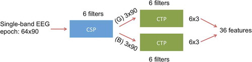
The above procedure was done in each frequency band separately to select a total of 36 features and the selected features from all 11 frequency bands were concatenated. Finally, a regularized-LDA classifier was trained [25,31].

3.5. Distance to Riemannian mean of spatial covariances (DRM-S)

Full-rank covariance matrices lie on a Riemannian manifold pertaining to the symmetric positive definite (SPD) matrices [15]. Let $A(n)$ be the set of all $n\times n$ SPD matrices. The Riemannian distance between $A_1\in A(n)$ and $A_2\in A(n)$ is defined as follows:

(6) ${\delta }_R(A_1,A_2)=||Log(A_1^{-1}{A}_2)|{|}_F=\left[\sum _{i=1}^{n}lo{g}^2{\lambda }_i\right]{ }^{1/2}$(6)

where ${\lambda }_i$ are the eigenvalues of $(A_1^{-1}{A}_2)$. Since $A_1$ and $A_2$ are both SPD, ${\lambda }_i$ are real positive (non-zero) values. Also, $||.|{|}_F$ represents the Frobenius norm and $Log(.)$ the matrix logarithm.

The mean of the SPD matrices $A_1,A_2,...,A_l$ on the Riemannian manifold is defined as follows [15]:

(7) $M(A_1,A_2,...,A_l)=argmi{n}_{X\in A(n)}\sum _{i=1}^l{\delta }_R^2(X,A_i).$(7)

There is no closed form solution for (7); however, it can be solved iteratively [34].

Based on the defined matrix relationships on the manifold, we propose a filter bank generalization of the minimum distance to Riemannian mean (MDM) classifier [26]. First, the Riemannian mean of the good and bad space covariances in each frequency band on the training set were estimated as described earlier. Next, in each frequency band, features were selected as the Riemannian distances to the Riemannian means of the good and bad classes. This resulted in a total of 22 features: 11 frequency bands ×2 good and bad classes. A logistic regression classifier was trained on the selected features [25]. We trained a logistic regression classifier for all Riemannian methods since we found that the distribution of features was far from a multivariate normal distribution.

3.6. Distance to Riemannian mean of temporal covariances (DRM-T)

This method is the temporal counterpart of the DRM-S method described previously. After the Riemannian mean of the good and bad time covariances in each frequency band on the training set were estimated, features were selected as the Riemannian distances to the Riemannian means of the good and bad classes. This resulted in a total of 22 features: 11 frequency bands ×2 good and bad classes. Logistic regression was trained on the selected features [25].

3.7. Distance to Riemannian mean of spatial and temporal covariances (DRM-ST)

This method combines spatial and temporal Riemannian geometry-based features by concatenating DRM-S and DRM-T features described in the previous two subsections. This resulted in a total of 44 features: 11 frequency bands ×2 good and bad classes ×2 time and space covariances. A logistic regression classifier was trained on the selected features [25].

3.8. Covariance-based Riemannian and Euclidean spatio-temporal classifier (CREST)

We combined DRM-ST and CSP-CTP to capture spatio-temporal features using both Riemannian and common spatial and temporal classifiers. We call this method CREST. For each classifier, we first calculated the signed distance of each trial to the decision hyperplane and applied a logistic function to estimate the probability of the trial belonging to the the good (or bad) class as the classifier score. Logistic regression was used to combine DRM-ST and CSP-CTP classifier scores [25].

3.9. Windowed-means (WM)

We compared our proposed methods with the windowed means method which is widely used for single-trial event-related potential (ERP) classification [11,14]. EEG data on each channel were bandpass filtered to 0.5–10 Hz as described earlier and epoched 50–950 ms after each cursor movement. We calculated the mean of the signal on each channel in 9 non-overlapping time windows, i.e. each covering 100 ms. Then, a regularized linear discriminant analysis (r-LDA) classifier was trained on the selected features [14,25,31].

3.10. CREST+WM

Finally, we combined DRM-ST, CSP-CTP and WM as well to compare with the WM classifier to determine whether WM and CREST capture different features. Logistic regression was used to combine DRM-ST, CSP-CTP and WM classifier scores as explained earlier [25].

4. Results and discussion

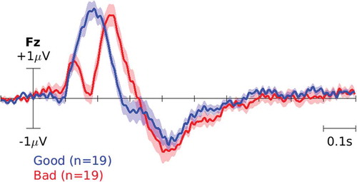
Figures 4 and 5 plot the event-related potential (ERP), i.e. the average EEG waveform time-locked to the cursor movement, for ‘Good’ and ‘Bad’ classes on channel Fz across participants for datasets I and II, respectively. For the plot, EEG data for each participant were high-pass filtered at 1 Hz and epoched −100 to 1000 ms time locked to each cursor movement. Then, the average waveform for each participant was calculated in each class. The solid lines on each plot represent the average across participants and the shaded color represents the standard error of the mean. Note that the two classes correspond to cursor movements toward/away from the target and our goal in this paper is to train a classifier to reliably distinguish among them after every cursor movement.

Figure 4. ERP in dataset I. The blue curve corresponds to the brain response to ‘good’ cursor movements, i.e. toward the target. The red curve, on the other hand, corresponds to the brain response to ‘bad’ movements, i.e. away from the target.

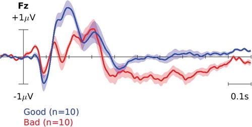
Figure 5. ERP in dataset II. The blue curve corresponds to the brain response to ‘good’ cursor movements, i.e. toward the target. The red curve, on the other hand, corresponds to the brain response to ‘bad’ movements, i.e. away from the target.

We compared the G/B classification performance in datasets I and II using CSP and DRM-S as well as CTP and DRM-T. Tables 1 and 2 report the average (first number in each entry) and standard error of the mean (second number in each entry) for classification accuracy over 10 instances of train-test for each participant in datasets I and II, respectively. On average, Riemannian methods perform better across participants and this difference is statistically significant for dataset I (paired-sample t-test, $p<0.03$). DRM-T performs significantly better than CTP in dataset II (paired-sample t-test, $p<0.01$). However, in this dataset, the difference between DRM-S and CSP is not statistically significant across participants.

Table 1. Dataset I: G/B classification accuracy using spatial and temporal features separately. Each table entry is the average classification accuracy (first number) together with the standard error of the mean (second number) over 10 instances of train-test for each participant. Riemannian methods outperform their counterparts and this difference is significant across participants (paired-sample t-test, $p<0.03$).

ID	CSP	DRM-S	CTP	DRM-T
A1	0.77/0.009	0.77/0.009	0.65/0.012	0.72/0.013
A2	0.74/0.017	0.74/0.011	0.64/0.015	0.68/0.014
A3	0.58/0.006	0.62/0.012	0.52/0.008	0.56/0.014
A4	0.74/0.007	0.76/0.010	0.63/0.011	0.64/0.011
A5	0.67/0.008	0.67/0.011	0.56/0.009	0.59/0.014
A6	0.73/0.006	0.72/0.010	0.62/0.011	0.68/0.014
A7	0.76/0.008	0.77/0.009	0.61/0.010	0.66/0.010
A8	0.66/0.016	0.71/0.009	0.66/0.013	0.71/0.007
A9	0.75/0.009	0.81/0.012	0.65/0.009	0.72/0.011
A10	0.67/0.016	0.71/0.015	0.66/0.012	0.69/0.012
Average	0.71/0.019	0.73/0.017	0.62/0.014	0.67/0.016

Table 2. Dataset II: G/B classification accuracy using spatial and temporal features separately. Each table entry is the average classification accuracy (first number) together with the standard error of the mean (second number) over 10 instances of train-test for each participant. DRM-T outperforms its counterpart and this difference is significant across participants (paired-sample t-test, $p<0.01$). However, the difference between CSP and DRM-S is not statistically significant.

ID	CSP	DRM-S	CTP	DRM-T
P1	0.76/0.015	0.74/0.010	0.57/0.017	0.61/0.012
P2	0.64/0.018	0.65/0.015	0.61/0.016	0.67/0.015
P3	0.87/0.016	0.83/0.013	0.72/0.014	0.74/0.014
P4	0.65/0.026	0.73/0.023	0.62/0.021	0.71/0.016
P5	0.67/0.019	0.62/0.026	0.53/0.023	0.63/0.024
P6	0.63/0.027	0.62/0.018	0.54/0.019	0.53/0.022
P7	0.72/0.017	0.68/0.022	0.54/0.017	0.52/0.017
P8	0.84/0.017	0.80/0.012	0.52/0.019	0.62/0.024
P9	0.58/0.024	0.58/0.020	0.50/0.027	0.46/0.025
P10	0.54/0.027	0.58/0.018	0.55/0.017	0.61/0.019
P11	0.71/0.020	0.73/0.025	0.66/0.023	0.73/0.022
P12	0.64/0.023	0.69/0.014	0.59/0.017	0.62/0.023
P13	0.57/0.016	0.57/0.025	0.52/0.018	0.56/0.015
P14	0.60/0.017	0.62/0.023	0.58/0.016	0.56/0.016
P15	0.66/0.025	0.66/0.025	0.61/0.016	0.60/0.021
P16	0.77/0.016	0.71/0.026	0.63/0.010	0.64/0.011
P17	0.65/0.024	0.68/0.015	0.57/0.032	0.62/0.024
P18	0.59/0.018	0.64/0.023	0.60/0.030	0.55/0.027
P19	0.64/0.021	0.70/0.016	0.60/0.011	0.64/0.013
Average	0.67/0.021	0.68/0.016	0.58/0.012	0.61/0.016

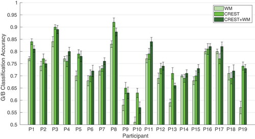
Tables 3 and 4 report the classification accuracy of the windowed-means method (WM) and our proposed spatio-temporal methods: DRM-ST and CSP-CTP, CREST and CREST+WM. We used paired-sample t-tests to compare the difference between WM and the other methods across participants for each dataset. CREST and CREST+WM outperform WM in both datasets (paired-sample t-test, $p<0.006$, which stays significant at the 0.05 threshold with Bonferroni correction for the number of tests).

Table 3. Dataset I: G/B classification accuracy comparing the proposed spatio-temporal methods and WM. Each table entry is the average classification accuracy (first number) together with the standard error of the mean (second number) over 10 instances of train-test for each participant. Significantly improved results across participants are represented in bold fonts (paired-sample t-test, $p<0.006$, which stays significant at the 0.05 threshold with Bonferroni correction for the number of tests, i.e. 4).

ID	WM	DRM-ST	CSP-CTP	CREST	CREST+WM
A1	0.75/0.006	0.79/0.009	0.80/0.009	0.82/0.005	0.83/0.006
A2	0.79/0.010	0.77/0.012	0.76/0.007	0.82/0.007	0.85/0.007
A3	0.68/0.010	0.60/0.016	0.61/0.011	0.63/0.008	0.68/0.010
A4	0.83/0.011	0.77/0.014	0.88/0.011	0.91/0.007	0.90/0.009
A5	0.73/0.011	0.67/0.011	0.77/0.008	0.79/0.008	0.80/0.012
A6	0.72/0.009	0.74/0.015	0.69/0.008	0.76/0.004	0.78/0.005
A7	0.79/0.011	0.77/0.008	0.76/0.009	0.81/0.007	0.84/0.008
A8	0.69/0.014	0.72/0.005	0.71/0.012	0.76/0.011	0.77/0.014
A9	0.75/0.008	0.81/0.010	0.73/0.010	0.82/0.006	0.84/0.010
A10	0.74/0.014	0.73/0.016	0.75/0.009	0.78/0.007	0.80/0.009
Average	0.75/0.015	0.74/0.019	0.75/0.023	0.79/0.022	0.81/0.019

Table 4. Dataset II: G/B classification accuracy comparing the proposed spatio-temporal methods and WM. Each table entry is the average classification accuracy (first number) together with the standard error of the mean (second number) over 10 instances of train-test for each participant. Significantly improved results across participants are represented in bold fonts (paired-sample t-test, $p<0.005$, which stays significant at the 0.05 threshold with Bonferroni correction for the number of tests, i.e. 4).

ID	WM	DRM-ST	CSP-CTP	CREST	CREST+WM
P1	0.77/0.008	0.72/0.019	0.83/0.017	0.84/0.012	0.81/0.013
P2	0.74/0.019	0.70/0.008	0.77/0.016	0.77/0.020	0.75/0.014
P3	0.84/0.021	0.83/0.011	0.90/0.013	0.90/0.010	0.89/0.016
P4	0.77/0.010	0.75/0.031	0.73/0.021	0.76/0.022	0.80/0.017
P5	0.70/0.020	0.66/0.025	0.79/0.018	0.79/0.017	0.78/0.022
P6	0.68/0.021	0.60/0.010	0.69/0.026	0.70/0.024	0.72/0.023
P7	0.72/0.017	0.67/0.011	0.73/0.017	0.73/0.012	0.76/0.014
P8	0.83/0.014	0.79/0.016	0.92/0.014	0.92/0.017	0.88/0.016
P9	0.58/0.023	0.54/0.025	0.64/0.024	0.65/0.023	0.63/0.024
P10	0.51/0.021	0.62/0.022	0.58/0.021	0.63/0.019	0.57/0.023
P11	0.77/0.017	0.76/0.021	0.78/0.017	0.79/0.023	0.84/0.018
P12	0.69/0.021	0.68/0.024	0.77/0.011	0.73/0.022	0.74/0.016
P13	0.59/0.015	0.58/0.013	0.72/0.024	0.71/0.023	0.66/0.010
P14	0.70/0.005	0.61/0.019	0.68/0.019	0.69/0.016	0.71/0.015
P15	0.68/0.016	0.66/0.019	0.67/0.024	0.70/0.020	0.73/0.016
P16	0.80/0.010	0.70/0.019	0.80/0.020	0.81/0.022	0.82/0.012
P17	0.80/0.009	0.68/0.021	0.77/0.025	0.77/0.020	0.82/0.019
P18	0.71/0.027	0.63/0.028	0.72/0.017	0.69/0.023	0.72/0.025
P19	0.57/0.026	0.71/0.021	0.73/0.009	0.74/0.017	0.73/0.016
Average	0.71/0.021	0.68/0.017	0.75/0.019	0.75/0.018	0.76/0.019

The difference in performance of DRM-ST and WM is not statistically significant for either of the datasets. However, CSP-CTP outperforms WM in dataset II and this difference is statistically significant (paired-sample t-test, $p<0.005$, which stays significant at the 0.05 threshold with Bonferroni correction for the number of tests), while the performance of CSP-CTP in dataset I is not statistically different from that of WM.

Figures 6 and 7 show WM, CREST and CREST+WM performance as bar plots for easier visualization.

Figure 6. WM, CREST and CREST+WM in dataset I. The bars and error bars represent the average classification accuracy and the standard error of the mean, respectively, i.e. first and second entries in Table 3 columns 2, 5 and 6.

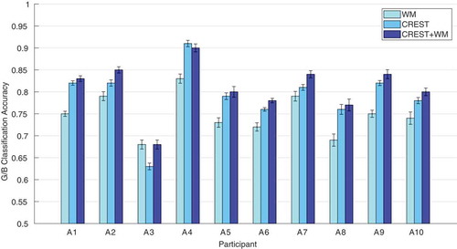
Figure 7. WM, CREST and CREST+WM in dataset II. The bars and error bars represent the average classification accuracy and the standard error of the mean, respectively, i.e. the first and second entries in Table 4 columns 2, 5 and 6.

5. Conclusions

We proposed spatio-temporal methods to classify the error-related brain activity and evaluated our results on two different datasets. The first dataset is from an active motor imagery BCI in which the user’s brain response to the BCI feedback is an implicit piece of information and using this information can improve the overall BCI performance [5]. We also evaluated our proposed methods on a passive BCI dataset in which participants were evaluating the movements of a cursor. In the latter, error-related brain activity is the core information to be classified even though it is not explicitly provided by the user.

We compared DRM-S and DRM-T that use Riemannian distances as features, with CSP and CTP methods, respectively, in their capacity for classifying feedback-related brain activity in response to BCI error. Our results show that on average across participants in both datasets, methods that use features from Riemannian geometry are more powerful when considering spatial or temporal features separately.

We also proposed methods to combine spatial and temporal features that use Riemannian distances (DRM-ST) and Euclidean geometry-based methods of common patterns (CSP-CTP). We also proposed to combine these two methods (CREST) and showed that this combined method outperforms the windowed-means (WM) method and the difference is statistically significant across participants in both datasets.

Abbreviations

Table

BCI	brain-computer interface
CREST	Covariance-based Riemannian and Euclidean spatio-temporal classifier
CSP	common spatial patterns
CTP	common temporal patterns
DRM	distance to Riemannian mean
EEG	electroencephalography
ERD	event-related desynchronization
ERP	event-related potential
G/B	good/bad
MI	motor imagery
pBCI	passive brain-computer interface
r-LDA	regularized linear discriminant analysis
WM	windowed-means

Acknowledgments

We would like to thank Laurens R. Krol and Thorsten O. Zander for sharing their dataset with us.

Disclosure statement

No potential conflict of interest was reported by the authors.

Additional information

Funding

This work was supported by the NSF [IIS 1219200, 1817226, 1528214]; DAAD [short-term research grant]; UC San Diego [Chancellor’s Research Innovation Scholarships G2171, G3155 and the Mary Anne Fox dissertation year fellowship]; NIH [5T32MH020002-18].

References

- Farwell LA, Donchin E. Talking off the top of your head: toward a mental prosthesis utilizing event- related brain potentials. Electroencephalogr Clin Neurophysiol. 1988;70(6):510–523.
- Wolpaw JR, McFarland DJ, Neat GW, et al. An EEG-based brain-computer interface for cursor control. Electroencephalogr Clin Neurophysiol. 1991;78(3):252–259.
- Pfurtscheller G, Brunner C, Schlögl A, et al. Mu rhythm (de) synchronization and EEG single-trial classification of different motor imagery tasks. NeuroImage. 2006;31(1):153–159.
- McFarland DJ, Miner LA, Vaughan TM, et al. Mu and beta rhythm topographies during motor imagery and actual movements. Brain Topogr. 2000;12(3):177–186.
- Mousavi M, Koerner AS, Zhang Q, et al. Improving motor imagery BCI with user response to feedback. Brain-Comput Interfaces. 2017;4(1–2):74–86.
- de Sa, V.R. An interactive control strategy is more robust to non-optimal classification boundaries. ICMI’12 pp 579-586 October 22-26, 2012 Santa Monica, California, USA. 2012. DOI: 10.1145/2388676.2388798.
- Chavarriaga R, Sobolewski A, Millán J. Errare machinale est: the use of error-related potentials in brain-machine interfaces. Front Neurosci. 2014;8:208.
- Schalk G, Wolpaw JR, McFarland DJ, et al. EEG-based communication: presence of an error potential. Clin Neurophysiol. 2000;111(12):2138–2144.
- Zander TO, Kothe C. Towards passive brain–computer interfaces: applying brain–computer interface technology to human–machine systems in general. J Neural Eng. 2011;8(2):025005.
- Krol L, Andreessen L, Zander T. Passive brain-computer interfaces: A perspective on increased interactivity. Brain-Comput Interfaces Handb. 2018;69–86.
- Zander TO, Krol LR, Birbaumer NP, et al. Neuroadaptive technology enables implicit cursor control based on medial prefrontal cortex activity. Proc Nat Acad Sci. 2016;113(52):14898–14903.
- Zander TO, Brönstrup J, Lorenz R, et al. Advances in physiological computing. In: Fairclough SH, Gilleade K, editors. Towards BCI-based implicit control in human–computer interaction. London: Springer; 2014. p. 67–90.
- Ferrez PW, Millán JD. Error-related EEG potentials generated during simulated brain–computer interaction. IEEE Trans Biomed Eng. 2008;55(3):923–929.
- Blankertz B, Lemm S, Treder M, et al. Single-trial analysis and classification of ERP componentsa tutorial. NeuroImage. 2011;56(2):814–825.
- Barachant A, Bonnet S, Congedo M, et al. Riemannian geometry applied to BCI classification. International Conference on Latent Variable Analysis and Signal Separation; Saint Malo, France. 2010. p. 629–636.
- Congedo M, Barachant A, Bhatia R. Riemannian geometry for EEG-based brain-computer interfaces; a primer and a review. Brain-Comput Interfaces. 2017;4(3):155–174.
- Kalunga EK, Chevallier S, Barthélemy Q, et al. Online SSVEP-based BCI using Riemannian geometry. Neurocomputing. 2016;191:55–68.
- Barachant A, Congedo M. A plug&play P300 BCI using information geometry. arXiv Preprint. 2014; https://arxiv.org/abs/1409.0107.
- Kalunga EK, Chevallier S, Barthélemy Q. Data augmentation in Riemannian space for brain-computer interfaces. STAMLINS; 2015.
- Mousavi M, de Sa VR. Spatio-temporal analysis of feedback-related brain activity in brain-computer interfaces. NeurIPS 2018 Workshop on modeling and decision-making in the spatiotemporal domain; Montreal, Canada; 2018.
- Mousavi M, de Sa VR. Towards elaborated feedback for training motor imagery brain computer interfaces. Proceedings of the 7th Graz Brain-Computer Interface Conference 2017; Graz, Austria; 2017. p. 332–337.
- Makeig S, Bell AJ, Jung TP, et al. Independent component analysis of electroencephalographic data. Advances in neural information processing systems; Denver, Colorado; 1996. p. 145–151.
- MATLAB. Natick, Massachusetts, United States: The MathWorks Inc.; 2018b.
- Delorme A, Makeig S. EEGLAB: an open source toolbox for analysis of single-trial EEG dynamics including independent component analysis. J Neurosci Methods. 2004;134(1):9–21. Available from: http://www.sciencedirect.com/science/article/pii/S0165027003003479
- Pedregosa F, Varoquaux G, Gramfort A, et al. Scikit-learn: machine learning in Python. J Mach Learn Res. 2011;12:2825–2830.
- Barachant A, Bonnet S, Congedo M, et al. Multiclass brain–computer interface classification by Riemannian geometry. IEEE Trans Biomed Eng. 2012;59(4):920–928.
- Blankertz B, Tomioka R, Lemm S, et al. Optimizing spatial filters for robust EEG single-trial analysis. IEEE Signal Process Mag. 2008;25(1):41–56.
- Lotte F, Bougrain L, Cichocki A, et al. A review of classification algorithms for EEG-based brain– computer interfaces: a 10 year update. J Neural Eng. 2018;15(3):031005.
- Noh E, Herzmann G, Curran T, et al. Using single-trial EEG to predict and analyze subsequent memory. NeuroImage. 2014;84:712–723.
- Schäfer J, Strimmer K. A shrinkage approach to large-scale covariance matrix estimation and implications for functional genomics. Stat Appl Genet Mol Biol. 2005;4(1):2194–6302.
- Ledoit O, Wolf M. Improved estimation of the covariance matrix of stock returns with an application to portfolio selection. J Empirical Finance. 2003;10(5):603–621.
- Ang KK, Chin ZY, Wang C, et al. Filter bank common spatial pattern algorithm on BCI competition IV datasets 2a and 2b. Front Neurosci. 2012;6:39.
- Yu K, Shen K, Shao S, et al. Common spatio-temporal pattern for single-trial detection of event- related potential in rapid serial visual presentation triage. IEEE Trans Biomed Eng. 2011;58(9):2513–2520.
- Moakher M. A differential geometric approach to the geometric mean of symmetric positive-definite matrices. SIAM Journal on Matrix Analysis and Applications. 2005;26(3):735–747.