Augmented Winter's method for forecasting under asynchronous seasonalities

Abstract

The method of Winters (1960) is one of the most well-known forecasting methodologies in practice. The main reason behind its popularity is that it is easy to implement and can give quite effective and efficient results for practice purposes. However, this method is not capable of capturing a pattern being emerged due to the simultaneous effects of two different asynchronous calendars, such as Gregorian and Hijri. We adapt this method in a way that it can deal with such patterns, and study its performance using a real dataset collected from a brewery factory in Turkey. With the same data set, we also provide a comparative performance analysis between our model and several forecasting models such as Winter’s (Winters 1960), TBAT (De Livera et al. 2011), ETS (Hyndman et al. 2002), and ARIMA (Hyndman and Khandakar 2008). The results we obtained reveal that better forecasts can be achieved using the new method when two asynchronous calendars exert their effects on the time-series.

Keywords:

• sales forecasting
• Ramadan effect
• asynchronous calendar effects
• exponential smoothing

1. Introduction

Typically, business or economics activities may change depending on calendar effects, namely weather conditions, holy days and festivities. Many countries in the world prefer to use the Gregorian calendar to organize and perform their business activities in synchronization with the other ones. Hence, the Gregorian calendar easily captures the pattern of seasons in nature, as well as the pattern of global festivities such as the New Year.

Although some countries use the Gregorian calendar for arranging their economic activities, they continue to follow different calendars for observing their own religious rituals and/or festivals, e.g., Ramadan, Easter, and Passover. In these religious festivities and holy days, the societies’ consumption habits distinguishably change based on their traditions. For instance, many consumers in Middle-East countries completely stop consuming alcoholic beverages during the Ramadan and tend to increase their soft drink consumptions. It is observed that in some markets, this increase reaches up to 50% (The Nielsen Company, 2015).

These religious festivities and holy days are scheduled on the Gregorian calendar months based on their unique calendars. As a result of this fact, they may not be observed in a fixed time period in the Gregorian calendar, even their dates may shift every year. The detection of this shifting effect on the sales levels would not be a simple task for the firms employing classical forecasting methods. Because many classical forecasting methods handle the time-series data with one seasonal character over the calendar in use. Correspondingly, with these naive methods, the sales forecasts would not be done effectively and accurately.

The main purpose of this work is to develop a new method for the situations where the effect of two asynchronous calendars -such as Gregorian and Hijri or Gregorian and Lunar- manifest themselves in the time-series simultaneously. To this end, we extend the work of Winters (1960) by incorporating a component that captures the second calendar effect. We also propose a guideline to determine the initial values of the parameters in our model. Lastly, we compare the performance of our new method with Winter’s (Winters, 1960), TBAT (De Livera, Hyndman, & Snyder, 2011), ETS (Hyndman, Koehler, Snyder, & Grose, 2002), and ARIMA (Hyndman & Khandakar, 2008) models, using a real dataset from a brewery in Turkey. To the best of our knowledge, this is the first attempt to introduce an adapted version of Winter’s method which recognize the effect of two asynchronous calendars simultaneously.

The rest of this work is organized as follows. In Section 2, we provide a detailed literature review on the forecasting methods that are close to our work. In Section 3, we briefly review the work of Winters (1960) and provide a discussion regarding the details of our new method. Besides that, in the same section, we propose a guideline for the choice of the smoothing parameters and initialization procedure. In Section 4, by using a case study at a major brewery in Turkey, we compare the forecasting performance of our new method with several well-known forecasting methods. Lastly, in Section 5, we summarize our results and main findings and give some suggestions for future research directions.

2. Literature review

The literature on the exponential smoothing forecasting methods is abundant. For the sake of clarity, we only restrict our attention to the ones relevant to our work. For further details on this research stream, we refer the reader to the review papers by Gardner (1985), Chatfield, Koehler, Ord, and Snyder (2001), Gardner (2006), and Syntetos, Boylan, and Disney (2009).

As one of the early studies in this research stream, Holt (2004) extends simple exponential smoothing to double exponential smoothing by introducing a linear trend component. Basically, with this extended method, the author combines the concept of exponential smoothing with the ability to track a linear trend in the dataset. On the other hand, Holt's method cannot track the series having any seasonal fluctuations. To deal with this problematic issue, Winters (1960) develops an elaboration of Holt's method. In that new model, a third equation is added to Holt's method to capture the seasonal dynamics of the data. Pegels (1969) provides an extension to these two methods, taking into account all combinations of trend and seasonal effects in additive and multiplicative forms. Brown (2004) introduces a new forecasting technique by integrating the exponential smoothing model with regressors whose coefficients are time varying. Newbold and Granger (1974) compare the forecasting performance of Box–Jenkins, Winter's, and step-wise regression methods using seven different time series. While conducting this comparison, the parameters being used in the forecasting methods are determined by the authors' own software. Chatfield (1978) reanalyzes the same seven series by using some subjective parameter adjustments. The author indicates that the computerized Winters forecasts can often be improved by subjective parameter adjustments and it would be much fairer if a comparison between Box–Jenkins and non-computerized Winter's methods is done. Chatfield and Yar (1988) discuss several problems being observed while implementing Winter's method, e.g. the choice of smoothing parameters and starting values, the normalization of seasonal indices and so on.

Although there is a vast literature on the detection of single-sourced seasonal fluctuations in a given calendar system, only a few papers attempt to address the joint effects of more than one calendar. Riazuddin et al. (2002) extend the classical ARIMA model to handle the effects of the Hijri calendar on the currency circulation in Pakistan. In that new model, the authors represent the second calendar effects with a set of dummy variables. With a similar technique, Yucel (2005) examines the effects of Ramadan on food prices in Turkey. Akmal et al. (2010) deal with how the changes in the consumer price index in Pakistan are affected by the existence of Ramadan. The authors emphasize that the effect of Ramadan on the consumer price index cannot be determined properly by using ARIMA models because of the data recording norms and inconsistency between the Hijri and Gregorian calendars. They attempt to cope with this problematic issue by conducting a scenario analysis based on three different datasets. Besides these studies, Lin et al. (2002), Seyyed, Abraham, and Al-Hajji (2005), and Rao et al. (2011) attempt to extend the classical ARIMA model to capture a second calendar effect being observed in time series.

Furthermore, De Livera et al. (2011) introduce a state space model for forecasting complex seasonal time series such as those with multiple seasonal periods, non-integer seasonality, and dual calendar effects. However, this model is overly complex with ARIMA error correction and Fourier representations of time varying coefficients. Due to this complexity, it is not easy to use that methodology for regular forecasting purposes. A similar solid statistical background is also used in a number of existing studies (e.g. Gould et al., 2008; Taylor, 2003, 2010; Taylor & Snyder, 2012; Tratar, Mojškerc, & Toman, 2016) which deal with exponential smoothing models to capture multiple seasonality patterns occurring due to an other calendar that is used out of the official calendar. Computational complexity, over parameterization, and/or the inability to accommodate both non-integer period and dual calendar effects can be attributed as the weakness of these models.

In supply chain management, in order to manage inventory levels that provide an acceptable level of service to customers, the demand forecasting is required on a regular basis for a very large number of products (Hyndman et al., 2002). The methods should, therefore, satisfy the requirements of being fast, flexible, user-friendly, and they are able to produce results, which are reliable, efficient, and easy to interpret by the user with a lack of advanced statistical knowledge. However, the conducted literature review shows that none of the existing studies satisfies both of these dimensions when the dual calendar effect comes into play in time series. Most of them are generally too complex to use in practice or they are not sufficient to capture the simultaneous effects of two asynchronous calendars.

To address this issue, we extend the work of Winters (1960) in a way that it can recognize the seasonalities being emerged in time series due to asynchronous calendars. The method that we develop in this study can be easily implemented in an Excel spreadsheet or a Matlab m-file. The optimization routines for the choice of parameters usually take a few seconds so the method facilitates the real-time analysis and forecasting of two seasonal patterns even though one of them originates from the second calendar. As well as ease of use, we believe that this contribution could have an impact on many forecasting settings in which the demand is shaped by the climate seasonality and cultural seasonality of the market.

3. Forecasting methods

In the following sections, we first review Winter's methods, and then, give the details of our new method.

3.1. Winter's method (WM)

Winters' method is a type of triple exponential smoothing and it is efficient when the dataset exhibits seasonal fluctuations and an increasing or decreasing linear trend over time. The most important advantage of this method is that it easy to update seasonal factors as new datasets become available (Nahmias & Cheng, 2009). The four equations that define this forecasting method are: (1) $\text{Level estimate:}{S}_t=\alpha \left(D_t/c_{t-N}\right)+(1-\alpha )(S_{t-1}-G_{t-1}),$(1) (2) $\text{Trend estimate:}{G}_t=\text{β}\left(S_t-S_{t-1}\right)+(1-\text{β})G_{t-1},$(2) (3) $\text{Seasonal estimate:}{c}_t=\gamma \left(D_t/S_t\right)+(1-\gamma )c_{t-N},$(3) (4) $\text{Forecast for }\tau \text{ periods ahead:}{F}_{t,t+\tau }=(S_t+G_t\tau )c_{t+\tau -N},$(4) where γ is a smoothing factor for the seasonality. α and β are smoothing factors for the level and trend, respectively. Also, t is an index denoting the time. The smoothing parameters denoting by α, β and γ are typically determined by minimizing an error measure of the fit, e.g. mean square error (MSE), mean absolute deviation (MAD) or mean absolute percentage error (MAPE). In practice, it has been using various advanced methods for choosing the smoothing and initialization parameters, e.g. Kalman filter, maximum likelihood estimation, and regression-based approaches. For a further detailed discussion on this subject, we refer the reader to the work of Hyndman, Koehler, Ord, and Snyder (2008).

3.2. Augmented Winter's method (AWM)

Winter's method allows the incorporation of seasonalities into forecasts. The assumption for this method is that there is a number of periods N, for a given $i=1,2,\dots ,N$ the elements of set $\{i+kN|k\in N\}$, show the same seasonal calendar character. Hence, the same seasonality factor comes into play every N periods. Typically, demand seasonalities are in synch with the Gregorian calendar. Temperature variations within the year specify the times for change of collections in the fashion industry due to their inherent effect in the demand pattern. The sales of ice cream or cold beverages are the most well-known examples for this situation, since they are designed to be consumed more when ambient temperature is higher. Similarly, there is additional demand for many types of good in well-known periods of the year due to festivities and accompanying gift-exchange traditions. All these phenomena with pronounced effect on demand patterns happen at the same period, each year. Hence, they can be captured within the framework of Winter's.

Winter's method suggests solution to handle time-series data with one seasonal character over the calendar in use. For this reason, there is a problem when two different calendars that are not synchronized come into play. The most prominent example of this is the asynchronization between the Gregorian and the Hijri calendars. With the influence of globalization as well as nature, these two calendars exert their influences simultaneously in many countries. The Gregorian calendar captures the rhythm of seasons in nature as well as the rhythm of – now global – festivities such as the New Year. In such a situation, there is a number of periods $N_1$, for a given $i=1,2,\dots ,N_1$ the elements of set $\{i+k{N}_1|k\in N\}$, show same seasonal primary calendar behavior. However, in Muslim countries (as in the example of Turkey), Islamic traditions also have profound effect in demand patterns. For instance, during the month of Ramadan, Muslims fast and their eating patterns are different to those during the rest of the year. Of particular significance is that alcohol consumption significantly drops during this month and soft beverage consumption shows an opposite characters. In this setting, the seasonality over the secondary calendar also comes into play every $N_2$ periods.

To capture simultaneous effects of two asynchronous calendars, we propose a new approach which we name as the Augmented Winter's method. In this methodology, we treat the data as a time series with multiple layers of seasonality in play. There is underlying linear model in the spirit of Holt. Then, the layer of first calendar seasonality is added just like in Winter. Finally, the new layer of second calendar seasonality is placed again via a multiplicative factor. In order to dynamically estimate the factors involved, we need to peel the data layer by layer.

In this method, we use two sets of seasonal factors to forecast the time series in a given period. The forecasting periods are according to the first calendar (Gregorian). The main difficulty is that the months of the two calendars do not usually coincide. For example, the month of Ramadan of Islamic calendar usually occurs at two consecutive months of the Gregorian calendar. Moreover, the number of days of Ramadan in each of these Gregorian months varies from year to year. Therefore, the new methodology has to partition the effect of Islamic calendar months to the specific Gregorian month. To address this issue, we postulate that the effect of secondary calendar months is distributed between the primary calendar months in proportion with the number of secondary calendar month days within each month.

Now, we can proceed to the process of peeling the second calendar effects out of the time series using the following equation: (5) $R_t=\sum _{i=1}^{N_2}\frac{D_t{h}_{it}}{k_i},$(5) where $h_{it}$ is the ratio of $i\text{th}$ secondary calendar month days in $t\text{th}$ primary calendar month to the total number of $i\text{th}$ primary calendar days, and $k_i$ is the coefficient for the $i\text{th}$ secondary calendar month. Actual observation in period t is denoted by $D_t$ whereas $N_2$ stands for the seasonality length of second calendar. We should also note that (6) $\sum _{t=1}^{N_1}{h}_{it}{d}_t^p=d_i^s,$(6) (7) $\sum _{i=1}^{N_2}{h}_{it}=1,$(7) where $d_t^p$ is the number of primary calendar days in the $t\text{th}$ primary calendar month and $d_i^s$ is the number of secondary calendar days in the $t\text{th}$ primary calendar month. In addition, seasonality length for primary calendar is denoted by $N_1$. The above equations imply that the days of $i\text{th}$ secondary calendar month are distributed on the primary calendar months with respect to the number of overlapped days within each month.

The smoothing factor for the secondary calendar seasonality is described by the following equation: (8) $k_i^{\prime }=\rho \left(\frac{\sum _{j\in S_R}{h}_{ij}{D}_j}{\sum _{j\in S_R}{h}_{ij}{R}_j}\right)+\left(1-\rho \right)k_i\text{where }{S}_R=\left\{j|h_{ij}>0\right\}.$(8) $k_i$ is the un-updated coefficient for the $i\text{th}$ secondary calendar month and $k_i^{\prime }$ is the updated coefficient for the $i\text{th}$ secondary calendar month. When the new data is available, $k_i^{\prime }$ is updated based on the secondary calendar smoothing factor $\rho ,\text{where }0\le \rho \le 1$.

Also, all of secondary calendar month factors are normalized so that their weighted averages are 1. The normalizing equation is explicitly expressed as follows: (9) $\frac{\sum _{i=1}^{N_2}{k^{\prime }}_i}{N_2}=1.$(9) Once the effect of the second calendar is taken out, the first calendar seasonalities are updated with (10) $c_t=\gamma \left(\frac{R_t}{S_t}\right)+\left(1-\gamma \right)c_{t-N_1},$(10) where γ is primary calendar seasonality smoothing factor.

Moreover, the sum of any $N_1$ successive seasonal factors should always be $N_1$. In other words, after estimating each seasonal factor, it is normalized with the most recent seasonal factors by using (11) $c_j=\left[\frac{c_j}{\sum _{i=t-N_1+1}^t{c}_i}\right]N_1\text{where }t-N_1+1\le j\le t.$(11) The fully deseasonalized series is now used to update level and trend estimates: (12) $S_t=\alpha \left(\frac{R_t}{c_{t-N_1}}\right)+\left(1-\alpha \right)\left(S_{t-1}+G_{t-1}\right),$(12) where α is smoothing factor for the level.

The new estimate of the trend component is simply defined as a smoothed sum of difference between two consecutive estimations of the deseasonalized level and the preceding trend estimate. Formally, it is: (13) $G_t=\text{β}\left(S_t-S_{t-1}\right)+\left(1-\text{β}\right)G_{t-1},$(13) where $0\le \text{β}\le 1$ is the trend smoothing constant, which determines the relative weight placed on the current estimation of the trend.

Lastly, the forecast made in period t for any future period $t+\tau$ is given by the following equation: (14) $F_{t,t+1}=\left(S_t+G_t\right)c_t\left(\sum _{i=1}^{N_2}{k}_i{h}_{it}\right).$(14) For this new method, we propose the following initialization procedure. First of all, a minimum of two full seasons ($2N_1$ periods) of historical data is required to initialize a set of seasonal factors. Then, we follow the procedure given below:

(1)	Calculate the sample means for the two separate seasons of data with, (15) $V_1=\frac{1}{N}\sum _{j=-2N_1+1}^{-N_1}{D}_j,$(15) (16) $V_2=\frac{1}{N}\sum _{j=-N_1+1}^0{D}_j,$(16) where the present period is $t=0$, and the past observations are identified by negative indices.
(2)	Estimate the initial slope $G_0$ and the level of the series $S_0$ with (17) $G_0=\frac{(V_2-V_1)}{N_1},$(17) (18) $S_0=V_2+G_0\left[\frac{N_1-1}{2}\right].$(18)
(3)	The raw seasonal indices are estimated for each initialization period as follows: (19) ${\hat{c}}_t=\frac{D_t}{V_i-\left[\frac{\left(N_1+1\right)}{2}-j\right]G_0},\text{where }-2N_1+1\le t\le 0,i=1,2.$(19)

Note that our raw estimates reflect the joint effects of the seasonalities of two asynchronous calendars. Hence, we need a more sophisticated approach to decompose the effect of each calendar's seasonality. Our suggestion for this problem is to solve the nonlinear least-square formulation given below: (20) $min\left[{\sum _{t=-2N_1+1}^{-N_1}\left({\hat{c}}_t-c_{t+N_1}\left(\sum _{i=1}^{N_2}{h}_{it}{k}_i\right)\right)}^2+{\sum _{t=-N_1+1}^0\left({\hat{c}}_t-c_t\left(\sum _{i=1}^{N_2}{h}_{it}{k}_i\right)\right)}^2\right],$(20) where $c_t\left(\sum _{i=1}^{N_2}{h}_{it}{k}_i\right)$ is the joint seasonal factor for period t of the second part of initialization set whereas $c_{t+N_1}\left(\sum _{i=1}^{N_2}{h}_{it}{k}_i\right)$ is the joint seasonal factor for the same period t of the first part of initialization set. With the equation given above, a proper set of seasonality factors and coefficients may not be obtained due to the fact that the solution of the nonlinear least square can yield negative values. In order to address this issue, the following constraints must be considered while solving the nonlinear least-square formulation: (21) $\sum _{t=1}^{N_1}{c}_t=N_1,$(21) (22) $\sum _{i=1}^{N_2}{k}_i=N_2,$(22) (23) $c_t>0\text{where }\in \{1,2,\dots ,N_1\},$(23) (24) $k_i>0\text{where }i\in \{1,2,\dots ,N_2\}.$(24) The above constraints imply the normality and positivity conditions on the factors. To minimize the above non-linear problem, one can use an off-the-shelf optimization software such as MATLAB, Python, or AIMMS.

3.3. An extension for augmented Winter's method

The flexible structure of the new method allows us to treat the effects of secondary calendar months separately, as well as giving an opportunity to examine the secondary calendar effect in a special structure such as a particular month and the others. In some cases, there might be only the effect of a single secondary calendar month on the actual data which is collected according to primary calendar. The Ramadan can be given as an example for this situation. In most of the Muslim countries, consumption habits are distinguishably affected due the holy Ramadan whereas the other months of Hijri calendar do not have a significant effect on the consumers. As a result of this fact, in a given dataset which is collected from this market structure, we might only see the effect of Ramadan. In such a case, the months can be grouped as Ramadan and Non-Ramadan ones. Hence, there will be only two seasonal factors for the second calendar effect, and they are denoted by $k_r$ and $k_o$. $k_r$ is the coefficient for Ramadan months whereas $k_o$ is the coefficient for Non-Ramadan months.

In this context, Equation stated in (5(5) $R_t=\sum _{i=1}^{N_2}\frac{D_t{h}_{it}}{k_i},$(5) ) is rephrased as follows: (25) $R_t=\left(\frac{D_t}{k_r}\right)r_t+\left(\frac{D_t}{k_o}\right)o_t,$(25) where $r_t$ ratio of Ramadan days in the current forecast period and $o_t$ ratio of Non-Ramadan days in the current forecast period.

By considering this modification, updating Equation (8(8) $k_i^{\prime }=\rho \left(\frac{\sum _{j\in S_R}{h}_{ij}{D}_j}{\sum _{j\in S_R}{h}_{ij}{R}_j}\right)+\left(1-\rho \right)k_i\text{where }{S}_R=\left\{j|h_{ij}>0\right\}.$(8) ) is revised and denoted as (26) ${k_r}^{\mathrm{\prime }}=\rho \left(\frac{\sum _{i\in S_R}{r}_i{D}_i}{\sum _{i\in S_R}{r}_i{R}_i}\right)+(1-\rho )k_r\text{where }0\le \rho \le 1\text{ and }{S}_R=\left\{i\right|r_i>0\},$(26) where ${k_r}^{\mathrm{\prime }}$ is the updated coefficient for the Ramadan month and $k_r$ is un-updated coefficient for the Ramadan month.

For the Non-Ramadan month, the equation will be (27) ${k_o}^{\mathrm{\prime }}=\rho \left(\frac{\sum _{i\in S_R}{o}_i{D}_i}{\sum _{i\in S_R}{o}_i{R}_i}\right)+(1-\rho )k_o\text{where }0\le \rho \le 1\text{ and }{S}_R=\left\{i\right|r_i>0\},$(27) where ${k_0}^{\mathrm{\prime }}$ is the updated coefficient for the Non-Ramadan month and $k_o$ is un-updated coefficient for the Non-Ramadan month.

Also, these two coefficients are normalized by using the following equation: (28) $11k_o+k_r=12.$(28) In such a case, the estimates for level, trend and the first calendar seasonalities remain same as defined in the previous section. The forecast equation in (14(14) $F_{t,t+1}=\left(S_t+G_t\right)c_t\left(\sum _{i=1}^{N_2}{k}_i{h}_{it}\right).$(14) ) is also adjusted as (29) $F_{t,t+\tau }=(S_t+\tau G_t)c_t(o_{t+\tau }{k}_o+r_{t+\tau }{k}_r).$(29) The nonlinear least-square equation (20(20) $min\left[{\sum _{t=-2N_1+1}^{-N_1}\left({\hat{c}}_t-c_{t+N_1}\left(\sum _{i=1}^{N_2}{h}_{it}{k}_i\right)\right)}^2+{\sum _{t=-N_1+1}^0\left({\hat{c}}_t-c_t\left(\sum _{i=1}^{N_2}{h}_{it}{k}_i\right)\right)}^2\right],$(20) ) for the initialization procedure is re-defined by considering these modifications. (30) $min\left[\sum _{t=-2N_1+1}^{-N_1}{\left({\hat{c}}_t-c_{t+12}\left(o_t{k}_o+r_t{k}_r\right)\right)}^2+\sum _{t=-N_1+1}^0{\left({\hat{c}}_t-c_t\left(o_t{k}_o+r_t{k}_r\right)\right)}^2\right]$(30)

4. Numerical results

In this section, we first describe the characteristics of our dataset, with a set of descriptive statistics. After that, using the dataset we have, we provide a comparative performance analysis between our model and Winter's, TBAT, ETS, and ARIMA models.

4.1. Dataset

This paper is motivated by a project undertaken at an important beer producer in Turkey. Their products are categorized in three dimensions: brand, package type, and package size. At the time of the study, a total of twelve beer brands are available in the Turkish market. These brands are on the market in three different packages (returnable bottle, non-returnable bottle, and can) and two sizes (35cc, 50cc). But, in this study we restrict our attention to only a specific returnable bottled beer which is the producer's bestselling product.

Our dataset consists of exactly 72 data points being collected between January 2008 and December 2013. The overall average and standard deviation of the monthly sales amounts are 8,601,398 and 5,395,557, respectively. In Figure 1, we present a line graph illustrating all data points in this dataset.

Figure 1. Monthly sales series.

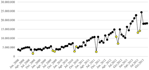
Three striking features of the sales data immediately come to light in Figure 1. First, there is an upward linear trend in the sales amounts from January 2008 to March 2012. Second, over the entire 12-month periods, the sales amounts show seasonal fluctuations with consistent peaks in summer months and declines in Ramadan (lighter colored markers). At the beginning of 2010, this product is relaunched with a new brand identity and a new bottle on the Turkish market. Besides that, the company has started a new price positioning for the product and supported it with intensive advertisements and sponsorship activities. Lastly, as a result of these efforts, a linear upward trend in the sales amounts after February 2010 has emerged. Furthermore, from Figure 1, it is seen that the average sales amount of the first 2 years, 2008 and 2009 are less than the average sales amount of the last 4 years, 2010, 2011, 2012 and 2013.

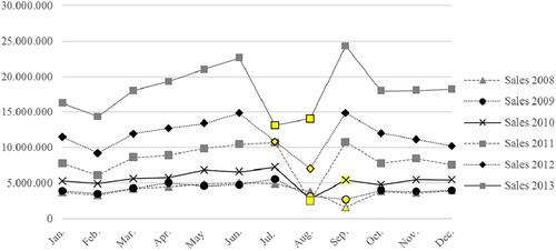
All of these observations are also confirmed with Figure (2) which separately depicts the monthly sales series for each year. The figure shows that the effect of Ramadan does not manifest itself in a single month of the Gregorian calendar (lighter colored markers are again Ramadan months). The lines connecting the months within the same year are parallel to each other. From this observation, we can infer that the average sales amount for each year is higher than the previous one. This means the existence of a linear upward trend in the dataset. Furthermore, from the figure, it is observed that the beer sales volumes exhibit a seasonal pattern. The patterns are obviously recurrent and consistent from year to year.

Figure 2. Yearly sales series.

4.2. Comparative performance analysis

Using the dataset introduced in the previous section, we compare the forecasting performance of our method with Winter's, ARIMA, TBAT, and ETS models.

We implement Winter's and ARIMA forecasting methods by using packages “forecast.HoltWinters” and ‘auto.arima’ in R. These two packages were developed by Hyndman et al. (2019). The model parameters are automatically determined by the corresponding package.

TBAT model is introduced by De Livera et al. (2011) for forecasting complex seasonal time series such as those with multiple seasonal periods, high-frequency seasonality, and dual-calendar effects. For more detailed information about the method, we refer the reader to the work of De Livera et al. (2011). The method is implemented by employing an R package called “forecast.tbats” (Hyndman et al., 2019). All corresponding parameters are determined by the package itself with a criterion of minimum AIC.

ETS model is proposed by Hyndman et al. (2002). This model is developed on a state space framework that includes all the exponential smoothing models and allows the computation of prediction intervals, likelihood, and model selection criteria. Hyndman et al. (2019) provide a full implementation of the model in an R Package called “forecast.ets”. We use this package to implement the model and let the package determines all the model parameters automatically with a criterion of minimum AIC.

We implement our new method in MATLAB and set the smoothing parameters $\alpha ,\text{β},\gamma$, and ρ with a criterion of minimum mean square error. To obtain the initial seasonal indices $c_i$ and the second calendar effects $k_o\text{and }{k}_r$, we solve Equation (30(30) $min\left[\sum _{t=-2N_1+1}^{-N_1}{\left({\hat{c}}_t-c_{t+12}\left(o_t{k}_o+r_t{k}_r\right)\right)}^2+\sum _{t=-N_1+1}^0{\left({\hat{c}}_t-c_t\left(o_t{k}_o+r_t{k}_r\right)\right)}^2\right]$(30) ) by employing the nonlinear least-squares optimization routine in MATLAB. In addition to the Ramadan factor, the effects of different Hijri months, like Muharram, Shawwal, and Dhul-Hajj, can also manifest itself in the Turkish beer market since Islamic societies in Turkey have many differences in the observance of festivities and mourning. This phenomenon has been controlled by having several extra models, and it has been observed that the effects of these months in the market are not as significant as Ramadan. Therefore, the models including the effects of different Hijri months are not given in this study. Due to this setting, we are not going to treat the months' of the second (Islamic) calendar separately, but we are going to classify them as Ramadan and the others.

We utilize the dataset by dividing it into two parts: (1) training set that covers the data points between January 2008 and December 2009 and (2) test set that covers the data points between January 2010 and December 2013. The training set is only used to determine the models' forecasting parameters. The model parameters we obtain with the training set is given in Table 1.

Table 1. The parameters of the models, obtained over the training set.

(a) WM and AWM models
Parameters	WM	AWM
α	0	0.25
β	0	0.10
γ	0.1	0.40
ρ	–	0.50
$k_o$	–	1.06
$k_r$	–	0.32
$c_1$	−31,875	0.87
$c_2$	−485,325	0.80
$c_3$	266,799	0.95
$c_4$	999,682	1.05
$c_5$	539,217	1.11
$c_6$	721,338	1.19
$c_7$	1,079,403	1.2
$c_8$	−219,923	0.92
$c_9$	−222,8118	1.23
$c_{10}$	−152,734	0.89
$c_{11}$	−365,136	0.89
$c_{12}$	−15,002	0.90
$S_0$	4,081,246	4,175,716
$G_0$	13,578	14,341
(b) ARIMA model
	ARIMA
AR coefficients	0
MA coefficients	0.45
Difference	0
(c) TBAT model
	TBAT
α	0.15
β	0.09
$m_1$	12.00
$m_2$	11.64
Damping Parameter	1.00
${\gamma }_1$ Values	$\{-0.0004,-0.0001\}$
${\gamma }_2$ Values	$\{0.0003,0.0003\}$
AR coefficients	−0.99
MA coefficients	0.69
(d) ETS model
	ETS
α	0.0001
l	3,982,827.33
σ	873,578.90

The test set is only used to provide a comparative performance analysis of the models fitted based on the training dataset. To this end, we define two accuracy measures: (1) Mean Squared Error (MSE), (31) $\text{MSE}=\frac{1}{n}\sum _{t=1}^n{(D_t-F_t)}^2,$(31) and (2) Mean Absolute Deviation (MAD), (32) $\text{MAD}=\frac{1}{n}\sum _{t=1}^n\left|D_t-F_t\right|,$(32) where $D_t$ is the actual observation and $F_t$ is the forecast obtained from a given method. Besides these two measures, for each model, the maximum error and square root of MSE are calculated. Winter's Method (WM) is used as a benchmark, and the relative change is defined by the following equation: (33) $\text{\%}\text{Change}=\frac{\text{Measure for forecasting method}-\text{Measure for WM}}{\text{Measure for WM}}100.$(33) A positive value in % Change implies that the benchmark method (WM) performs better than the compared method whereas a negative value signifies an improvement compared to WM.

Considering one-step-ahead forecasts, the accuracy measures of three forecasting methods are given in Table 2. These measures are calculated only over the test set. Besides that, Figure 3(a–e) are depicted in order to give a visual impression about the performance of the forecasting methods. Each of these figures illustrates the actual data points in the test set, the fitted values obtained with the corresponding forecast model whose parameters determined based on the training set, and the corresponding residuals.

Figure 3. Actual-Fitted-Residual graphs obtained by using the corresponding forecasting method: (a) WM, (b) AWM, (c) ETS, (d) ARIMA and (e) TBAT.

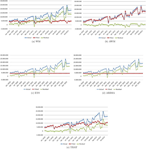
Table 2. Accuracy measures obtained over the test set.

	WM	AWM	% Change	TBAT	% Change
MSE	68.63${\text{e}}^{12}$	1.22${\text{e}}^{12}$	−98.22%	20.55${\text{e}}^{12}$	−70.06%
$\sqrt{\text{MSE}}$	8,284,251	1,105,021	−86.66%	4,533,242	−45.28%
MAD	6,590,239	934,123	−85.83%	3,059,544	−53.57%
Max. Error	21,859,253	2,583,203	−86.66%	14,927,318	−31.71%
		ETS	% Change	ARIMA	% Change
MSE		75.31${\text{e}}^{12}$	9.74%	74.87${\text{e}}^{12}$	9.10%
$\sqrt{\text{MSE}}$		8,678,374	4.76%	8,653,062	4.45%
MAD		7,024,568	6.59%	6,994,639	6.14%
Max. Error		20,340,496	−6.95%	20,308,864	−7.09%

The results show that in terms of all considered accuracy measures, ETS and ARIMA models are inferior to other ones. This is due to the fact that both models need a larger training dataset to capture the seasonal patterns, trend, and level in the dataset. On the other hand, the results reveal that AWM improves all considered accuracy measures when compared to WM. Our new method leads to a reduction in MSE and MAD of 98.22% and 85.83%, respectively. With the use of AWM, a significant improvement in the maximum error is also achieved, i.e. it is reduced by 86.66%. Although TBAT has successful results compared to WM, it is inferior to AWM in terms of all performance measures. TBAT leads to a 70.06% reduction in MSE whereas it reduces the maximum error by 31.71%. As it is understood from the results, our new method is capable of capturing the shifting second calendar effect, as well as the first calendar effect. Hence, it generates superior results compared to the others.

5. Conclusion

The method of Winters (1960) is one of the most well-known forecasting methodologies in practice. The main reason behind its popularity is that it is easy to implement and can give quite effective and efficient results for practice purposes. The method is capable of capturing a linear upward or downward trend in the data, as well as a cyclic seasonal factor originating from the calendar in use. However, it is not efficient at capturing a pattern being emerged due to the simultaneous effects of two different asynchronous calendars, such as Gregorian and Islamic (Hijri). We adapt this method in a way that it can accommodate the effects of two different asynchronous calendars. This adapted method, which is called Augmented Winters Method (AWM), involves an additional seasonal index, and an extra smoothing equation for the new seasonal index.

In order to illustrate the performance of our new forecasting method, a real life time series, which is provided by a leading beer factory in Turkey, is utilized. The performance of the new method is also compared with Winter's, ARIMA, ETS, and TBAT models. Our results show that ETS, ARIMA, and TBAT models are inferior to AWM. This can be attributed to the fact that they need a larger training dataset to capture the seasonal, trend, and level parameters properly and/or are a type of over-parameterized model. The results also reveal that in terms of all considered accuracy measures, our new method performs better than WM. This is mainly due to the fact that WM does not capture the second calendar effect very well.

This study can be extended in several ways. We determine the initial parameters for our new method by using a very naive method. The initialization procedure we use in this study can be improved with machine learning and artificial intelligence techniques. The forecasts to be obtained with such techniques, most probably, would be more accurate and effective and the true power of the proposed model would be better reflected. This is left for future work. The method we proposed in this study is implemented to a single dataset since we could not find any other dataset where two asynchronous calendars' effects are observed. Observing the performance of the new method over the different datasets would definitely be better for the generalization of our results.

Acknowledgments

We would like to thank the reviewers for their constructive feedback that helped us to improve the manuscript.

Disclosure statement

No potential conflict of interest was reported by the author(s).

References

- Akmal, M. , & Abbasi, M. U. , et al. (2010). Ramadan effect on price movements: Evidence from Pakistan (Technical report). State Bank of Pakistan, Research Department.
- Brown, R. G. (2004). Smoothing, forecasting and prediction of discrete time series. New York, NY: Courier Corporation.
- Chatfield, C. (1978). The Holt-Winters forecasting procedure. Applied Statistics , 27 (3), 264–279.
- Chatfield, C. , Koehler, A. B. , Ord, J. K. , & Snyder, R. D. (2001). A new look at models for exponential smoothing. Journal of the Royal Statistical Society: Series D (The Statistician) , 50 (2), 147–159.
- Chatfield, C. , & Yar, M. (1988). Holt-Winters forecasting: Some practical issues. The Statistician , 37 (2), 129–140.
- De Livera, A. M. , Hyndman, R. J. , & Snyder, R. D. (2011). Forecasting time series with complex seasonal patterns using exponential smoothing. Journal of the American Statistical Association , 106 (496), 1513–1527.
- Gardner, Jr., E. S. (1985). Exponential smoothing: The state of the art. Journal of Forecasting , 4 (1), 1–28.
- Gardner, Jr., E. S. (2006). Exponential smoothing: The state of the art–Part II. International Journal of Forecasting , 22 (4), 637–666.
- Gould, P. G. , Koehler, A. B. , Ord, J. K. , Snyder, R. D. , Hyndman, R. J. , & Vahid-Araghi, F. (2008). Forecasting time series with multiple seasonal patterns. European Journal of Operational Research , 191 (1), 207–222.
- Holt, C. C. (2004). Forecasting seasonals and trends by exponentially weighted moving averages. International Journal of Forecasting , 20 (1), 5–10.
- Hyndman, R. , Koehler, A. B. , Ord, J. K. , & Snyder, R. D. (2008). Forecasting with exponential smoothing: The state space approach . Berlin: Springer Science & Business Media.
- Hyndman, R. J. , Athanasopoulos, G. , Bergmeir, C. , Caceres, G. , Chhay, L. , O'Hara-Wild, M. , … Wang, E. (2019). Package “forecast”. Online. Retrieved from https://cran.r-project.org/web/packages/forecast/forecast.pdf.
- Hyndman, R. J. , & Khandakar, Y. (2008). Automatic time series forecasting: The forecast package for R. Journal of Statistical Software , 27 (3), 1–22.
- Hyndman, R. J. , Koehler, A. B. , Snyder, R. D. , & Grose, S. (2002). A state space framework for automatic forecasting using exponential smoothing methods. International Journal of Forecasting , 18 (3), 439–454.
- Lin, J.-L. , & Liu, T.-S. , et al. (2002). Modeling lunar calendar holiday effects in Taiwan. Taiwan Economic Forecast and Policy , 33 (1), 1–37.
- Nahmias, S. , & Cheng, Y. (2009). Production and operations analysis . California, CA: McGraw-Hill New York.
- Newbold, P. , & Granger, C. W. (1974). Experience with forecasting univariate time series and the combination of forecasts. Journal of the Royal Statistical Society. Series A (General) , 137 (2), 131–165.
- Pegels, C. C. (1969). Exponential forecasting: Some new variations. Management Science , 15 (5), 311–315.
- Rao, N. H. , Bukhari, S. K. H. , & Jalil, A. , et al. (2011). Detection and forecasting of Islamic calendar effects in time series data: Revisited (Technical report).
- Riazuddin, R. , et al. (2002). Detection and forecasting of Islamic calendar effects in time series data (Technical report). State Bank of Pakistan, Research Department.
- Seyyed, F. J. , Abraham, A. , & Al-Hajji, M. (2005). Seasonality in stock returns and volatility: The Ramadan effect. Research in International Business and Finance , 19 (3), 374–383.
- Syntetos, A. A. , Boylan, J. E. , & Disney, S. M. (2009). Forecasting for inventory planning: A 50-year review. Journal of the Operational Research Society , 60 (sup1), S149–S160.
- Taylor, J. W. (2003). Short-term electricity demand forecasting using double seasonal exponential smoothing. Journal of the Operational Research Society , 54 (8), 799–805.
- Taylor, J. W. (2010). Triple seasonal methods for short-term electricity demand forecasting. European Journal of Operational Research , 204 (1), 139–152.
- Taylor, J. W. , & Snyder, R. D. (2012). Forecasting intraday time series with multiple seasonal cycles using parsimonious seasonal exponential smoothing. Omega , 40 (6), 748–757.
- The Nielsen Company (2015, July). The Ramadan effect – reflecting on food consumption in United Arab Emirates and Saudi Arabia (Technical report).
- Tratar, L. F. , Mojškerc, B. , & Toman, A. (2016). Demand forecasting with four-parameter exponential smoothing. International Journal of Production Economics , 181 , 162–173.
- Winters, P. R. (1960). Forecasting sales by exponentially weighted moving averages. Management Science , 6 (3), 324–342.
- Yucel, E. M. (2005). Does Ramadan have any effect on food prices: A dual-calendar perspective on the Turkish data (Technical report).