LDL-AURIS: a computational model, grounded in error-driven learning, for the comprehension of single spoken words

ABSTRACT

A computational model for the comprehension of single spoken words is presented that builds on an earlier model using discriminative learning. Real-valued features are extracted from the speech signal instead of discrete features. Vectors representing word meanings using one-hot encoding are replaced by real-valued semantic vectors. Instead of incremental learning with Rescorla-Wagner updating, we use linear discriminative learning, which captures incremental learning at the limit of experience. These new design features substantially improve prediction accuracy for unseen words, and provide enhanced temporal granularity, enabling the modelling of cohort-like effects. Visualisation with t-SNE shows that the acoustic form space captures phone-like properties. Trained on 9 h of audio from a broadcast news corpus, the model achieves recognition performance that approximates the lower bound of human accuracy in isolated word recognition tasks. LDL-AURIS thus provides a mathematically-simple yet powerful characterisation of the comprehension of single words as found in English spontaneous speech.

KEYWORDS:

• Spoken word recognition
• error-driven learning
• Widrow-Hoff learning rule
• naive discriminative learning
• linear discriminative learning

1. Introduction

In linguistics, the hypothesis of the duality of patterning of language (also known as the dual articulation of language) has attained axiomatic status. Language is considered to be a symbolic system with a two-level structure. One level concerns how meaningless sounds pattern together to form meaningful units, the words and morphemes of a language. The other level is concerned with the calculus of rules that govern how words and morphemes can be assembled combinatorially into larger ensembles (Chomsky & Halle, 1968; Hockett & Hockett, 1960; Licklider, 1952; Martinet, 1967).

Accordingly, most cognitive models of spoken word recognition (henceforth SWR) such as the TRACE model (McClelland & Elman, 1986), the COHORT model (Marslen-Wilson, 1987), the SHORTLIST model (Norris, 1994), the Neighborhood Activation Model (Luce et al., 2000), the SHORTLIST-B model (Norris & McQueen, 2008), and the FINE-TRACKER model (Scharenborg, 2008), all posit two levels of representation and processing, a lexical and a prelexical level. The prelexical level is put forward to enable the system to convert the continuous varying input audio signal into discrete non-varying abstract units, sequences of which form the lexical units functioning in the higher-level combinatorics of morphology and syntax. The main motivation for having an intermediate phone-based representation is that phones are judged to be crucial for dealing with the huge variability present in the speech signal. Thus, at the prelexical level, the speech signal is tamed into phones, and it is these phones that can then be used for lexical access (Diehl et al., 2004; McQueen, 2005; Norris & McQueen, 2008; Phillips, 2001).

Although traditional SWR models posit a prelexical level with a finite number of abstract phone units, the psychological reality of an intermediate segmental level of representation has been long debated (see Pisoni & Luce, 1987, for a review, and Port & Leary, 2005, for linguistic evidence). Furthermore, the exact nature of these phone units is admittedly underspecified (McQueen, 2005); unsurprisingly, SWR models define their prelexical representation in very different ways. SHORTLIST and SHORTLIST-B work with phones and phone probabilities, TRACE posits multi-dimensional feature detectors that activate phones, and FINE-TRACKER implements articulatory-acoustic features. Unfortunately, most models remain agnostic on how their prelexical representations and phone units can actually be derived from the speech signal. As observed by Scharenborg and Boves (2010),

“the lack of a (cognitively plausible) process that can convert speech into prelexical units not only raises questions about the validity of the theory, but also complicates attempts to compare different versions of the theory by means of computational modelling experiments”.

Nevertheless, many modellers assume that some intermediate phone level is essential. Dahan and Magnuson (2006), for instance, motivates the acceptance of a prelexical level by the theoretical assumption that separation of tasks in a two-stage system engenders cognitive efficiency because of the restrictions imposed on the amount of information available for smaller mappings at each stage. The only model that argues against a mediating role of phones is the Distributed Cohort Model (Gaskell & Marslen-Wilson, 1997, 1999), which is motivated in part by the experimental research of Warren (1970, 1971, 2000), which provides evidence that the awareness of phonemes is a post-access reconstruction process.¹

In many SWR models, word meanings, the ultimate goal of lexical access (Harley, 2014), are represented at a dedicated lexical layer. A review of the different ways in which meanings have been represented in the literature is given by Magnuson (2017), here, we focus on two dominant approaches.

Firstly, in localist approaches, as implemented by the LOGOGEN model (Morton, 1969), TRACE, SHORTLIST, FINE-TRACKER, Neighborhood Activation Model, PARSYN (Luce et al., 2000), and DIANA (ten Bosch et al., 2015), the mental lexicon provides a list of lexical units that are either symbolic units or unit-like entries labelled with specifications of the sequence of phones against which the acoustic signal has to be matched. Once a lexical unit has been selected, it then provides access to its corresponding meaning.

Secondly, in distributed approaches, adopted by models such as the Distributed Cohort Model and EARSHOT (Magnuson et al., 2020), a word's meaning is represented by a numeric vector specifying the coordinates of that word in a high-dimensional semantic space.² The status of phone units within these approaches is under debate. The Distributed Cohort Model argues that distributed recurrent networks obviate the need for intermediate phone representations, and hence this model does not make any attempt to link patterns of activation on the hidden recurrent layer of the model to abstract phones. By contrast, the deep learning model of Magnuson et al. (2020) explicitly interprets the units on its hidden layer as the fuzzy equivalents in the brain of the discrete phones of traditional linguistics.

All these very different models of SWR provide theories of the mental lexicon that have several problematic aspects. First, the input to most models of auditory word recognition is typically a symbolic approximation of real conversational speech. The only models that work with real speech are FINE-TRACKER (Scharenborg, 2008, 2009), DIANA, and EARSHOT. Of these models, FINE-TRACKER and DIANA are given clean laboratory speech as input, whereas EARSHOT limits its input to a list of 1000 words generated by a text-to-speech system. However, normal daily conversational speech is characterised by enormous variability, and the way in which words are produced often diverges substantially from their canonical dictionary pronunciation. For instance, a survey of the Buckeye corpus (Pitt et al., 2005) of spontaneous conversations recorded at Columbus, Ohio (Johnson, 2004) revealed that around 5% of the words are spoken with one syllable missing, and that a little over 20% of words have at least one phone missing, compared to their canonical dictionary forms (see also Ernestus, 2000; Keune et al., 2005). It is noteworthy that adding entries for reduced forms to the lexicon has been shown not to afford better overall recognition (Cucchiarini & Strik, 2003). Importantly, canonical forms do not do justice to how speakers modulate fine phonetic detail to fine-tune what they want to convey (Hawkins, 2003). Plag et al. (2017) have documented that the acoustic duration of word-final [s] in English varies significantly in the mean depending on its inflectional function (see also Tomaschek et al., 2019). Thus, if the speech signal were to be reduced to just a sequence of categorical units, such as the canonical phones, then large amounts of information present in the speech signal would be lost completely. As a consequence, models of SWR have to take on the challenge of taking real spontaneous speech as input. Only by doing so can the models truly investigate the cohort effect of lexical processing that assumes the process of spoken word recognition starts by gradually winnowing out incompatible words with the incoming stream of audio and succeeds once a uniqueness point in the input is reached (Marslen-Wilson, 1984; Marslen-Wilson & Welsh, 1978).

Second, models of SWR typically do not consider how their parameter settings are learned. Models such as TRACE and SHORTLIST make use of connection weights that are fixed and set by hand. The Bayesian version of SHORTLIST estimates probabilities on the basis of a fixed corpus. The parameters of the Hidden Markov Model underlying DIANA are likewise tuned by hand and then frozen. Connectionist models such as the Distributed Cohort Model and EARSHOT are trained incrementally, and hence can be considered learning models. In practice, these models are trained until their performance is deemed satisfactory, after which the model is taken to characterise an adult word recognition system. However, vocabulary size is known to increase over the lifetime (Keuleers et al., 2015; Ramscar et al., 2014) and ideally the dynamics of life-long learning should be part of a learning model of lexical processing. By contrast, current deep learning models typically require massive amounts of data. The general practice to attend to this issue is availing the model of many passes through the training data, and training is typically terminated when a sweet spot has been found where prediction accuracy under cross-validation has reached a local maximum. Since further training would lead to a reduction in accuracy, training is terminated and no further learning can take place. Importantly, when small and/or simplified datasets are used for training, they can easily overfit the data and may not generalise well.

Third, all the above models work with a fixed lexicon. When morphologically complex words are included, as for instance in SHORTLIST-B, no mechanisms are implemented that would allow the model to recognise out-of-vocabulary inflected or derived words that have in-vocabulary words as their base words. In other words, these models are all full-listing models (Butterworth, 1983).

Finally, all the above-mentioned models of SWR require complex modelling architectures, minimally requiring three layers, one layer representing speech input, one or more intermediate layers, and a layer with lexical units. In what follows, we build on a very different approach to lexical processing (Baayen et al., 2019), in which high-dimensional representations for words' forms are mapped directly onto high-dimensional representations for words' meanings. Mathematically, this is arguably the simplest way in which one can model how word forms are understood. An important research question in this research programme is to see how far this very simple approach can take us before breaking.

A first proposal for modelling auditory comprehension within this general approach was formulated by Arnold et al. (2017). Several aspects of their and our approach to auditory word recognition are of special interest from a cognitive perspective. These authors developed discrete acoustic features from the speech signal that are inspired by the signal pre-processing that takes place in the cochlea. These features were used within a naive discriminative learning model (Baayen et al., 2011), which was trained on the audio of words extracted from a corpus of German spontaneous speech. Model recognition accuracy for a randomly selected set of 1000 audio tokens was reported to be similar to the lower bound of human recognition accuracy for the same audio tokens.

The model of Arnold et al. (2017) has several shortcomings (see, e.g. Nenadić, 2020), which we will discuss in more detail below. In this study, we introduce a new model, LDL for AUditory word Recognition from Incoming Spontaneous speech (LDL-AURIS), that enhances the original model in several ways. Our revised model affords substantially improved prediction accuracy for unseen words. It also provides enhanced temporal granularity so that now cohort-like effects emerge naturally. Visualisation of the form space using t-SNE (van der Maaten & Hinton, 2008) shows that the new acoustic features that we developed better capture phone-like similarities and differences. Thus, the very simple formalisation of the relation between form and meaning given by LDL-AURIS provides a promising tool for probing human auditory comprehension. Nonetheless, LDL-AURIS, similar to the model of Arnold et al. (2017), is a model of single word recognition and receives the audio data of one isolated token at a time. The words are harvested from real conversational speech to stay as faithful as possible to how language is used.

As our new model builds on previous modelling work using Naive Discriminative Learning (NDL; Baayen et al., 2011) and Linear Discriminative Learning (LDL; Baayen et al., 2019), the next section provides an introduction to these modelling approaches. Although the present study restricts itself to modelling the comprehension of uninflected words, handling inflection is a pivotal advantage of the general framework of LDL. The subsequent section then describes the changes we implemented in order to improve both model performance for SWR and to make the model cognitively more plausible.

2. Previous modelling of SWR with NDL and LDL

2.1. Informal characterisation of NDL and LDL

The NDL and LDL models are grounded in error-driven learning as formalised in the learning rules of Rescorla and Wagner (1972) and Widrow and Hoff (1960). These two learning rules are closely related, and are actually identical under specific parameter settings. As we shall see below, both implement a form of incremental multiple linear regression, and both rules can be also seen as simple artificial neural networks with an input layer with cues, an output layer with outcomes, and no hidden layers (the terminology of cues and outcomes is borrowed from Danks, 2003). Cues are sublexical form features, and outcomes are values on the axes of a high-dimensional semantic space. Error-driven learning as formalised by Rescorla and Wagner (1972) has proven to be fruitful for understanding both animal learning (Bitterman, 2000; Gluck & Myers, 2001; Rescorla, 1988) and human learning (Ellis, 2006; Nixon, 2020; Olejarczuk et al., 2018; Ramscar et al., 2014; Ramscar & Yarlett, 2007; Ramscar et al., 2010; Siegel & Allan, 1996).

Statistically, a model trained with the Rescorla-Wagner learning rule is a classifier that is trained to predict whether or not a specific outcome is present. Naive discriminative learning extends this single-label classifier to a multiple-label classifier by having the model learn to predict multiple outcomes in parallel. For instance, Baayen et al. (2011) built a model for Serbian case-inflected nouns, and for the noun ženama taught the model to predict three labels (classes): WOMAN, PLURAL, and DATIVE (see Sering et al., 2018, for mathematical details). Naive discriminative learning has been used successfully for modelling, e.g. unprimed visual lexical decision latencies for both simple and morphologically complex words (Baayen et al., 2011; Baayen, Milin, et al., 2016), masked priming (Milin et al., 2017), non-masked morphological priming (Baayen & Smolka, 2020), the acoustic duration of English syllable-final [s] (Tomaschek et al., 2019), and early development of speech perception in infants (Nixon & Tomaschek, 2020, 2021).³ Arnold et al. (2017) and Shafaei-Bajestan and Baayen (2018) used naive discriminative learning to train classifiers for SWR for German and English respectively. Both models made use of cues that were extracted from the audio signal. Below, we discuss how this was done in further detail, and in this study we will show how their method of signal preprocessing can be enhanced. Importantly, both studies took as input the audio files of words extracted from spontaneous conversational speech.

Linear Discriminative Learning (Baayen et al., 2019) relaxes the assumption made by Naive Discriminative Learning that outcomes are coded as present (1) or absent (0). By allowing outcomes to be real numbers, words' meanings can now be represented using vector representations from distributional semantics (Landauer & Dumais, 1997; Mikolov et al., 2013). Mathematically, LDL models are equivalent to multivariate multiple regression models. Baayen et al. (2019) tested their model on 130,000 words extracted from 20 h of speech sampled from the NewsScape English Corpus (Uhrig, 2018a), which is based on the UCLA Library Broadcast NewsScape. Chuang et al. (2020) trained an LDL model on the audio files of the MALD database (Tucker et al., 2019), and used this model to predict the acoustic durations and auditory lexical decision latencies to the auditory nonwords in this database.

The Rescorla-Wagner and Widrow-Hoff learning rules implement incremental error-driven learning that uses gradient descent (for mathematical details, see the next section). Alternatively, one can estimate the “endstate” or “equilibrium state” of learning. This endstate provides the connection strengths between cues and outcomes for an infinite number of tokens sampled from the training data. Danks (2003) provides equilibrium equations for the endstate of learning with the Rescorla-Wagner learning rule. Table 1 provides an overview of how NDL and LDL set up representations and error-driven learning. How exactly the discrete (NDL, previous LDL models) or real-valued (LDL, this study) cue vectors are defined is independent of the learning algorithms. Below, we discuss in further detail the choices made in the present study for representing form and meaning. In the next section, we provide details on the mathematics underlying NDL and LDL. Readers who are not interested in the technical details can proceed to Section 2.3.

Table 1. Overview of NDL and LDL.

	NDL	LDL
Cues	Discrete (1/0)	Discrete (1/0)/real valued
Outcomes	Discrete (1/0)	Real-valued
Incremental learning	Rescorla-Wagner	Widrow-Hoff
Endstate of learning	Danks equilibrium equations	Multivariate multiple regression

2.2. Formal model definitions

The error-driven learning algorithms of Rescorla-Wagner, Widrow-Hoff, and LDL regression are supervised learning algorithms that learn the weights on the connections between cue (input) and outcome (output) values in double-layer artificial neural networks with the objective of minimising the discrepancy between the desired outcome and the system's predicted outcome. The first two models achieve this mapping by updating the weights step by step as learning events are presented to the model. The third algorithm calculates the final state of learning using the matrix algebra of multivariate multiple regression. We begin with formally defining the task of iterative learning from a training set.

Definition 2.1

learning

Given

• scalars m, n, and p,

• a set $C=\{c_i\}$ for $i\in 1\cdot \cdot m$, where $c_i$ is a cue,

• a set $O=\{o_j\}$ for $j\in 1\cdot \cdot n$, where $o_j$ is an outcome,

• a set $X=\{{\mathit{x}}_t\}$ for $t\in 1\cdot \cdot p$, where ${\mathit{x}}_t$ is a row vector over C,

• a set $Y=\{{\mathit{y}}_t\}$ for $t\in 1\cdot \cdot p$, where ${\mathit{y}}_t$ is a row vector over O,

• a labelled training sequence of learning events $T=(e_t)$ for $t\in 1\cdot \cdot p$, where $e_t=({\mathit{x}}_t,{\mathit{y}}_t)$ is a learning event,

compute a mapping $P:X\to Y$ such that $P({\mathit{x}}_t)\approx {\mathit{y}}_t$.

We first consider incremental learning. Here, we use a double-layer fully-connected feed-forward network architecture for learning the mapping P from the training sequence T (Figure 1). This network has m neurons in the input layer, n neurons in the output layer with activation function f, and $m\times n$ connections from the input layer to the output layer. Input vector ${\mathit{x}}_t=[x_{ti}{]}_{1\times m}$ stores $x_{ti}$, the value that input neuron $c_i$ assumes at trial t, and output vector ${\mathit{y}}_t=[y_{tj}{]}_{1\times n}$ stores $y_{tj}$, the value that output neuron $o_j$ assumes at trial t. The weight on the connection from $c_i$ to $o_j$ at trial t is denoted as $w_{tij}$.

Figure 1. A double-layer fully-connected feed-forward neural network during learning at trial t.

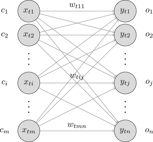
At trial t, an output neuron $o_j$ receives m input values $x_{ti}$ on afferent connections with associated weights $w_{tij}$, and combines the input values into the net input activation $a_{tj}$ $a_{tj}=\sum _{i=1}^m{x}_{ti}{w}_{tij}.$In neural networks, a variety of activation functions f are available for further transforming this net input activation. In our model, f is always the identity function, but f can be chosen to be any Riemann integrable function. Thanks to using the identity function, in our model, the neuron's predicted output ${\hat{y}}_{tj}$ is simply ${\hat{y}}_{tj}=f(a_{tj})=a_{tj}.$The error for a neuron is defined as the difference between the desired target output and the output produced by the neuron: $E_{tj}=y_{tj}-{\hat{y}}_{tj}.$The error for the whole network is defined as sum of squared residuals divided by two: (1) $E_t=\sum _{j=1}^n\frac{1}{2}(y_{tj}-{\hat{y}}_{tj}{)}^2.$(1) Both the Rescorla-Wagner and the Widrow-Hoff learning rules try to find the minimum of the function $E_t$ using gradient descent (Hadamard, 1908), an iterative optimisation algorithm for finding a local minimum of a function. The algorithm, at each step, moves in the direction of the steepest descent at that step. The steepest descent is defined by the negative of the gradient. Therefore, at each trial, it changes the weight on the connection from $c_i$ to $o_j$, $w_{tij}=w_{(t-1)ij}+\mathrm{\Delta }{w}_{tij},$proportional to the negative of the gradient of the function $E_t$: $\mathrm{\Delta }{w}_{tij}\propto -\frac{\mathrm{\partial }{E}_t}{\mathrm{\partial }{w}_{tij}}.$Thus, assuming a constant scalar η, often referred to as the learning rate, the changes in weights at time step t are defined as $\mathrm{\Delta }{w}_{tij}=-\eta \frac{\mathrm{\partial }{E}_t}{\mathrm{\partial }{w}_{tij}}$ or, (2) $\mathrm{\Delta }{w}_{tij}=\eta (y_{tj}-{\hat{y}}_{tj})f^{\prime }(a_{tj})x_{ti}$(2) (see Appendix A.1 for a proof of (2), which is known as the Delta rule and as the Least Mean Square rule). After visiting all learning events in the training sequence, the state of the network is given by a weight matrix $\mathit{W}=[w_{(t=p)ij}{]}_{m\times n}=[w_{ij}{]}_{m\times n}$. The requested mapping P in Definition 2.1 is given by element-wise application of the activation function f to the net input activations. Since in our model, f is the identity function, we have that $P({\mathit{x}}_t)=f\circ ({\mathit{x}}_t\mathit{W})={\mathit{x}}_t\mathit{W}={\hat{\mathit{y}}}_t.$Widrow-Hoff learning assumes that ${\mathit{x}}_t$ and ${\mathit{y}}_t$ are real-valued vectors in ${\mathbb{R}}^m$ and ${\mathbb{R}}^n$ respectively. Rescorla-Wagner learning is a specific case of the general definition of 2.1 in which the cues and outcomes of the model can only take binary values, representing the presence or absence of discrete features in a given learning event. Rescorla-Wagner also restricts the activation function f to be the identity function (see Appendix A.2 for further details).

Instead of building up the network incrementally and updating the weights for each successive learning event, we can also estimate the network, or its defining matrix $\mathit{W}$ in one single step, taking all training data into account simultaneously. To do so, we take all learning trials together by stacking the input vectors ${\mathit{x}}_t$ in matrix $\mathit{X}=[x_{ti}{]}_{p\times m}$ and stacking the output vectors ${\mathit{y}}_t$ in matrix $\mathit{Y}=[y_{tj}{]}_{p\times n}$, for all i,j,t. We are interested in finding a mapping that transforms the row vectors of $\mathit{X}$ into the row vectors of $\mathit{Y}$ as accurately as possible. Here, we can fall back on regression modelling. Analogous to the standard multiple regression model $\mathit{y}=\mathit{X}\mathit{\beta }+\mathit{\epsilon },$we can define a multivariate multiple regression model (3) $\mathit{Y}=\mathit{X}\mathit{B}+\mathit{E}$(3) with errors $\mathit{\epsilon }$ and $\mathit{E}$ being i.i.d. and following a Gaussian distribution. The multivariate regression model takes a multivariate predictor vector ${\mathit{X}}_{t.}$, weights each predictor value by the corresponding weight in ${\mathit{B}}_{.t}$, resulting in a vector of predicted values ${\hat{\mathit{Y}}}_{t.}$. Assume that $\mathit{X}$ is an m-by-m square matrix with determinant $det(\mathit{X})\ne 0$. Then there exists a matrix ${\mathit{X}}^{-1}$, the inverse $\mathit{X}$, such that $\mathit{X}{\mathit{X}}^{-1}={\mathit{X}}^{-1}\mathit{X}={\mathit{I}}_m,$where ${\mathit{I}}_m$ is the identity matrix of size m. Then, the matrix of coefficients $\mathit{B}$ is given by $\mathit{B}={\mathit{X}}^{-1}\mathit{Y}$(see Appendix A.3 for illustration). In practice, $\mathit{X}$ is singular, i.e. its determinant is 0, and the inverse does not exist. In this case, the Moore-Penrose (Penrose, 1955) generalised matrix inverse $X^{+}$ can be used $\mathit{B}={\mathit{X}}^{+}\mathit{Y}.$Calculating the Moore-Penrose pseudoinverse is computationally expensive, and to optimise calculations the system of equations $\mathit{Y}=\mathit{X}\mathit{B}$ can be recast as (4) $\begin{array}{rl}\mathit{Y}& =\mathit{X}B\\ ({\mathit{X}}^T\mathit{X}{)}^{-1}{\mathit{X}}^T\mathit{Y}& =({\mathit{X}}^T\mathit{X}{)}^{-1}{\mathit{X}}^T\mathit{X}\mathit{B}\\ ({\mathit{X}}^T\mathit{X}{)}^{-1}{\mathit{X}}^T\mathit{Y}& =\mathit{B}.\end{array}$(4) The inverse is now required for the smaller matrix ${\mathit{X}}^T\mathit{X}$. In this study, we estimate $\mathit{B}$ using the Moore-Penrose pseudoinverse. Returning to our model for SWR, we replace the multivariate multiple regression equation (3(3) $\mathit{Y}=\mathit{X}\mathit{B}+\mathit{E}$(3) ) with (5) $\mathit{Y}=\mathit{X}\mathit{W},$(5) where $\mathit{W}$, the matrix defining the connection weights in the network, replaces the matrix of coefficients $\mathit{B}$. We will show below that $\mathit{W}$ provides us with a network that has reached the endstate of learning, where its performance accuracy is maximal.

The twin models of NDL and LDL can now be characterised mathematically as follows. NDL's incremental engine uses Rescorla-Wagner, LDL's incremental engine is Widrow-Hoff.⁴ For the endstate of learning, NDL uses the equilibrium equations of Danks (2003), which yield exactly the same weight matrix as the one obtained by solving (5(5) $\mathit{Y}=\mathit{X}\mathit{W},$(5) ). LDL's endstate model uses the multivariate multiple regression model using (4(4) $\begin{array}{rl}\mathit{Y}& =\mathit{X}B\\ ({\mathit{X}}^T\mathit{X}{)}^{-1}{\mathit{X}}^T\mathit{Y}& =({\mathit{X}}^T\mathit{X}{)}^{-1}{\mathit{X}}^T\mathit{X}\mathit{B}\\ ({\mathit{X}}^T\mathit{X}{)}^{-1}{\mathit{X}}^T\mathit{Y}& =\mathit{B}.\end{array}$(4) ).

Given a trained model with weight matrix $\mathit{W}$, the question arises of how to evaluate the model's predictions. For a learning event $e_t$, NDL returns the outcome $o_j$ with the highest value in the predicted outcome vector: $\underset{o_j}{\mathrm{argmax}}{\mathit{x}}_t\mathit{W}.$LDL calculates the Pearson correlation coefficients of the predicted outcome vector ${\hat{\mathit{y}}}_t$ and all gold standard outcome vectors ${\mathit{Y}}_t$, resulting in a vector of correlations ${\mathit{r}}_t=[r({\hat{\mathit{y}}}_t,{\mathit{Y}}_t){]}_{1\times p}$, and returns the word type for the token with the highest correlation value $\underset{{\mathit{y}}_t}{\mathrm{argmax}}{\mathit{r}}_t.$

2.3. Challenges for spoken word recognition with LDL

Previous studies using LDL (Baayen et al., 2019) and NDL (Shafaei-Bajestan & Baayen, 2018) for English auditory word recognition report good accuracy on the training data: 34% and 25%, respectively. However, the latter study documents that accuracy is halved under cross-validation but is still superior to that of Mozilla Deep Speech.⁵ It is therefore possible that LDL is substantially overfitting the data and that its cross-validation accuracy is by far not as good as its accuracy on the training data. To place this question in perspective, we first note that models for visual word recognition as well as models such as TRACE and SHORTLIST have worked with invariable symbolic input representations for words' forms. However, in normal conversational speech, the wave forms of different tokens of the same linguistic word type are never identical, and often vary substantially. Thus, whereas models working with symbolic representations can dispense with cross-validation, models that take real speech as input cannot be evaluated properly without cross-validation on unseen acoustic tokens of known, previously encountered, linguistic word types. We note here that gauging model performance on seen data is also of interest, as for a psycholinguistic model the question of how well the model remembers what it has learned is of intrinsic interest.

A related issue is whether LDL, precisely because it works with linear mappings, may be too restricted to offer the desired accuracy under cross-validation. Thus, it is an empirical question whether the hidden layers of deep learning can be truly dispensed with. If hidden layers are indeed required, then this would provide further support for the position argued for by Magnuson et al. (2020) that phonemes are essential to SWR and that they emerge naturally in a deep learning network's hidden layers (but see Gaskell & Marslen-Wilson, 1997, 1999, for counterevidence). Furthermore, even if LDL were to achieve good performance under cross-validation, using a linear mapping from acoustic features to semantic vectors, then how would the model account for the evidence for phone-like topological maps in the cortex (see, e.g. Cibelli et al., 2015)?

There is one other aspect of the question concerning potential overfitting that requires further investigation. It is well known that deep learning networks run the risk of overfitting, too. Often there is a sweet spot as the model is taken through the dataset repeatedly to optimise its weights, at which accuracy under cross-validation reaches a local maximum. With further training, accuracy on the training set then increases, whereas accuracy under cross-validation decreases – the hallmark of overfitting. Weitz (2019) observed that the loss function for an LSTM network distinguishing between 100 word types in our dataset repeatedly jolts sharply out of local minimum beyond a threshold for training. This raises the question of whether the endstate of learning, as used by LDL, is actually optimal when accuracy is evaluated under cross-validation. If it is suboptimal, then incremental learning in combination with cross-validation is preferable under the assumption that there is a sweet spot where accuracy on the training data and on unseen data is properly balanced.

A very different challenge to NDL and LDL comes from classical cognitive models of SWR that provide predictions over time for the support that a target word and its closest competitors receive from the incoming auditory stimulus (Marslen-Wilson, 1984), irrespective of whether words are considered in isolation as in TRACE or in sentence context as in SHORTLIST. The temporal granularity of the previous NDL and LDL models (Arnold et al., 2017; Baayen et al., 2019; Shafaei-Bajestan & Baayen, 2018), however, is too coarse to be able to provide detailed predictions for cohort-like effects. An important goal of the present study is to develop enhanced acoustic features that enable the model to predict the time-course of lexical processing with greater precision.

A final challenge that we address in this study is whether further optimisation of model performance is possible by enhancing the representation of words' meanings. Whereas models such as the Distributed Cohort Model and EARSHOT assign randomly-generated semantic representations to words, and DIANA uses localist representations for word meanings, Baayen et al. (2019) and Chuang et al. (2020) made use of semantic vectors (aka word embeddings, see Gaskell & Marslen-Wilson, 1999, for a similar approach) derived from the TASA corpus (Ivens & Koslin, 1991; Landauer et al., 1998) using the algorithm described in Baayen, Milin, et al. (2016) and Baayen et al. (2019).⁶ The TASA corpus, with 10 million words, is very small compared to the volumes of texts that standard methods from machine learning such as word2vec (Mikolov et al., 2013) are trained on (typically billions of words). Although our TASA-based semantic vectors perform well (see Long, 2018, for an explicit comparison with word2vec), they may not be as discriminable as desired, thereby reducing model performance. We therefore investigated several ways in which the choice of semantic vectors affects model performance.

In what follows, we first address the issues surrounding potential overfitting (Section 4). We then introduce enhanced acoustic features that afford greater temporal granularity (Section 5). The question of what semantic representations are optimal is investigated in Section 6. Section 7 brings the results from the preceding sections together and defines and tests our enhanced model for SWR, LDL-AURIS.

3. Data

The data used in the current study is a subset of the UCLA Library Broadcast NewsScape,⁷ a massive library of audiovisual TV news recordings along with the corresponding closed captions. Our subset from the year 2016 was taken from the NewsScape English Corpus (Uhrig, 2018a). It consists mainly of US-American TV news and talk shows, and includes 500 audio files that are successfully aligned with their closed captions for at least 97% of their audio word tokens using the Gentle forced aligner.⁸ The real success rate is most likely substantially lower than the self-reported 97% but is still expected to be around 90% for these files. One of the reasons for the lower actual performance is that closed captions are often not accurate transcripts of the spoken words. Still, the error rate is an acceptable price to pay for being able to work with a large authentic dataset. The aligner provides alignment at word and phone level. Subsequently, we automatically extracted the relatively clean 30-second long audio stretches where there is speech with little background noise or music, following Shafaei-Bajestan and Baayen (2018). 2287 of such segments were randomly sampled to comprise a total of 20 h of audio including non-speech sounds.

This dataset contains 131,372 uninflected non-compound word tokens of 4741 word types.⁹ All words are lower-cased and stop words are retained. The left panel of Figure 2 shows that words in this dataset roughly follow Zipf's law. The durations of audio word tokens add up to a total of 9.3 h with an average word duration of 254 ms ($\mathrm{SD}=154$, range: 10–1480). One-third of the tokens are approximately between 100 to 200 ms long. The longest audio token belongs to an occurrence of the word “spectacular”. Gentle's temporal resolution is 10 ms, and sometimes when there are extreme phonetic reductions or other alignment problems, sounds and thus even monophonemic words are assigned a duration of 10 ms. In our dataset, instances of the words “are”, “a”, “i”, “or”, “oh”, “eye”, “e”, “owe”, “o” have been assigned this length. Due to the low overall number of such cases, they will not receive any separate treatment, even though a duration of 10 ms is highly implausible. Appendix B provides some examples of such imperfect alignments.

Figure 2. The dataset shows similar statistical trends to those of the English language's lexicon. The left panel shows that word frequency decreases linearly with Zipf word rank in a double logarithmic plane, a necessary condition for a power law relation. The right panel shows that word duration follows a lognormal distribution.

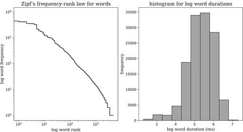
The right panel of Figure 2 shows that word duration has an approximately lognormal distribution, an observation in accordance with previous findings for the distribution of American-English spoken word lengths (French et al., 1930; Herdan, 1960). This dataset is employed in all simulations presented throughout the present study. All models are trained and tested on single word tokens as given by the word boundaries provided by the aligner.

The choice to model isolated word recognition is motivated primarily by the practical consideration that modelling word recognition in continuous speech is a hard task, and that a focus on isolated word recognition makes the task more manageable. It can be observed that, in general, this task is similar to a multiclass classification problem, classifying auditory instances into one of the thousands of word types possible. This is not to say that isolated word recognition is a simple task. On the contrary, Pickett and Pollack (1963) and Pollack and Pickett (1963) demonstrated long ago that spoken words isolated from conversational speech are difficult to recognise for human listeners: American English speech segments comprising one word with a mean duration of approximately 200 ms are, on average, correctly identified between 20% to 50% of the times by native speakers, depending on speaking rate. Arnold et al. (2017) reported similar recognition accuracy percentages from 20% to 44% for German stimuli with an average duration of 230 ms. Interestingly, deep learning networks are also challenged by the task of isolated word recognition. Arnold et al. (2017) reported that the Google Cloud Speech API correctly identified only 5.4% of their stimuli. Likewise, Shafaei-Bajestan and Baayen (2018) found that Mozilla Deep Speech, an open-source implementation of a state-of-the-art speech recognition system, performed with an accuracy around 6%, lagging behind the accuracy of their NDL model with around 6–9%. However, the lower performance of deep learning is likely to be due to the pertinent models being trained on much larger datasets; in other words, the NDL models had the advantage of being fine-tuned to the specific data on which they were evaluated.

A further reason for focussing on isolated words at this stage of model development is that, with the exception of the shortlist models (Norris, 1994; Norris & McQueen, 2008), computational models in psycholinguistics have also addressed single word recognition. While Weber and Scharenborg (2012) have argued that recognising individual words in utterances is a precondition for understanding, we would maintain that the evidence to the contrary is overwhelming. Besides the obvious problems for such an approach that arise from the small percentage of identifiable words discussed in the previous paragraph, Baayen, Shaoul, et al. (2016) have argued that not only is such segmentation unnecessary for discrimination but that it is also inefficient. Furthermore, evidence from language acquisition research seems to indicate that entire chunks are often learned first and understood although the segmentation into words will take place later in development (see, e.g. Tomasello, 2003).

By focussing on isolated word recognition, we are also setting ourselves the task to clarify how much information can be extracted from words' audio signals. Deep learning models for speech recognition depend heavily on language models, and current deep learning implementations may, given the above-mentioned results, underestimate the mileage that can be made by careful consideration of the rich information that is actually present in the acoustic signal. It is noteworthy that it has been argued that in human (continuous) SWR the acoustic input has overwhelming priority (Gaskell & Marslen-Wilson, 2001; Magnuson, 2017) (but see Cooke, 2006, for counterevidence).

4. Learning with Rescorla-Wagner, Widrow-Hoff, and multivariate linear regression

The aim of this section is to clarify how incremental learning and the endstate of learning compare. Of specific interest is whether the endstate of learning is suboptimal compared to some intermediate stage reached through incremental learning. We also consider how working with discrete semantic vectors (with sparse binary coding of the presence of lexemes) as opposed to real-valued semantic vectors affects results.

4.1. Method

For incremental learning with gradient descent training, we need to specify a learning rate η (set to 0.001 in our simulations) and the number of iterations n through the data (set to 1 in previous studies using NDL, but varied in the present simulations). There is no need for choosing η and n when using the matrix inversion technique for estimating the endstate of learning. Inversion of large matrices can become prohibitively slow for very large datasets. Fortunately, there have been major developments in optimising the algorithms for computations of the pseudo-inverse in computer science (see Horata et al., 2011; Lu et al., 2015, for example), and for the present data, all pseudo-inverse matrices are straightforward to calculate.

Table 2 summarises the four set-ups that we considered by crossing the training method (incremental vs. endstate of learning) with the method for representing word meanings (NDL vs. LDL). For all simulations, the acoustic input is represented by the Frequency Band Summaries features developed by Arnold et al. (2017). For incremental learning with gradient descent for Rescorla-Wagner and Widrow-Hoff we made use of the Python library pyndl (Sering et al., 2020). For endstate estimation with matrix inversion, we developed original code packaged in Python library pyLDLauris, available in the supplementary materials.

Table 2. The four models considered in the simulations.

	Outcomes
Training method	Lexomes	Semantic vectors
Gradient descent	Rescorla-Wagner (NDL)	Widrow-Hoff (LDL)
Matrix inversion	NDL classifier (Danks, 2003)	LDL multivariate multiple regression

The input to pyndl is a sequence of learning events consisting of a set of cues and a set of outcomes. For NDL, the set of outcomes provides identifiers for the lexomes realised in the speech signal. Lexomes are defined as identifiers of, or pointers to, distributional vectors for both content words and grammatical functions such as PLURAL and PAST (Baayen, Milin, et al., 2016; Milin et al., 2017). Mathematically, the set of outcome lexomes is represented by means of a binary vector with bits set to 1 for those lexomes that are present in the word, and set to 0 for all other words (see Baayen & Smolka, 2020, for further details). Since in the present study we only consider uninflected monomorphemic words and uninflected derived words, and no compound words (see Baayen et al., 2019, for further details), the set of lexomic outcomes reduces to an identifier for a word's content lexome, and the corresponding semantic vector reduces to a vector with only 1 bit on (one-hot encoding). For the present dataset, the lexomic vectors have a dimensionality of 4741 – the number of unique word types.

For simulations using LDL, one-hot encoding is replaced by real-valued semantic vectors. The word embeddings are supplied to the training algorithms in the form of a matrix. The word identifier for the lexome in the standard input for the algorithm is used to extract the appropriate semantic vector from this matrix. The semantic vectors that we consider here are obtained from a subset of semantic vectors derived from the TASA corpus as described in Baayen et al. (2019), comprising 12,571 word types and morphological functions, each of which is associated with a real-valued vector of length 4609.¹⁰ Henceforth, we will refer to this semantic space as the TASA1 space. It contains vectors for all of the word types in our dataset.

For both NDL and LDL, we need a matrix specifying the acoustic features for each of the word tokens in our dataset. From the features extracted for a word from the audio signal, following Arnold et al. (2017), an input form vector is constructed with 1s for those acoustic features that are present in the word and 0s for those features that are not realised in the word. The form vectors for the dataset ($N=131,372$) have a dimensionality of 40,578 – the number of unique FBS features. Thus, our form vectors are extremely sparse. Defining vector sparsity as the ratio of zero-valued elements to the total number of elements in the vector, our form vectors have an average sparsity of 0.99 ($\mathrm{SD}=0.009$).

Thus, for both NDL and LDL, we have two matrices, a $131,372\times 40,578$ form matrix $\mathit{C}$, and a semantic matrix $\mathit{S}$ which is of dimension $131,372\times 4741$ for NDL and of dimension $131,372\times 4609$ for LDL, irrespective of whether or not learning is incremental. For non-incremental learning, the weight matrix (or matrix of coefficients) is obtained by solving the system of equations defined by $\mathit{C}$ and $\mathit{S}$ as explained in the preceding section. For incremental learning, learning proceeds step by step through all the learning events defined by the rows of the matrices. This process is repeated for each of the n iterations over the data.

4.2. Results

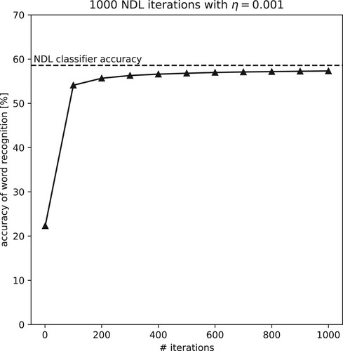
Our first simulation experiment takes as starting point the NDL model of Shafaei-Bajestan and Baayen (2018), which maps the (discrete) auditory cues onto lexomic semantic vectors. As this study also considered only uninflected words, the task given to the model is a straightforward classification task. Figure 3 presents the classification accuracy on the training data at the endstate of learning by means of a horizontal dashed line. The solid line presents model accuracy when the Rescorla-Wagner learning rule is used. The first data point represents accuracy after one iteration, the value reported by Shafaei-Bajestan and Baayen (2018). Subsequent datapoints represent accuracy after 100, 200, …, 1000 iterations through the dataset. Importantly, the endstate accuracy emerges as the asymptote of incremental learning. Apparently, it is not the case that there is a sweet spot at which incremental learning should be terminated in order to avoid overfitting.

Figure 3. NDL learning curve, using one-hot encoded semantic vectors. NDL accuracy using the Rescorla-Wagner learning rule approaches the asymptotic equilibrium state of the NDL classifier.

In the second simulation experiment, we replaced one-hot encoding of semantic vectors with the distributional vectors of the TASA1 semantic space. Figure 4 illustrates that training with the Widrow-Hoff learning rule to discriminate between words' semantic vectors also slowly moves towards the endstate asymptote. However, the overall accuracy of this model is substantially reduced to only 33.7% at equilibrium. Although again incremental learning with the Widrow-Hoff learning rule is confirmed to be incremental regression, with estimated coefficients asymptoting to those of a multivariate multiple regression analysis, the drop in accuracy is unfortunate. Why would it be that moving from one-hot encoded semantic vectors to distributional vectors is so detrimental to model performance?

Figure 4. Widrow-Hoff learning curve, using semantic vectors derived from TASA. Widrow-Hoff accuracy approaches the asymptotic state approximated by an LDL model, but accuracy is substantially reduced compared to Figure 3.

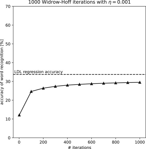
A possible reason is that the classification problem with one-hot encoded vectors is easier. After all, one-hot encoded vectors are all completely orthogonal: the encoding ensures that each word's semantic vector is fully distinct and totally uncorrelated with the semantic vectors of all other words. One-hot encoding should therefore make the task of the classifier easier, as semantic vectors have been made optimally discriminable. With empirical semantic vectors, by contrast, words will be more similar to other words, and this makes them more difficult to learn. To test this explanation, we replaced the TASA1 vectors in the previous experiment by random vectors sampled from a uniform distribution over $[0,1)$. The resulting pattern of learning is virtually identical to that shown in Figure 3 (figure not shown). Thus, as long as semantic vectors are orthogonal, incremental learning with Rescorla-Wagner and with Widrow-Hoff produces exactly the same results.

The above simulations quantified accuracy on the training set. To gauge the extent to which the models overfit, we split the data into a training and a test set with a 9:1 ratio. A weight matrix is trained on the training set using LDL that predicts the real-valued semantic vectors (of Section 6.3) from FBS features. The matrix is applied once to the training set and another time to the test set. These accuracy numbers are marked by two horizontal dashed lines in Figure 5. Another weight matrix is trained incrementally on the training set using Widrow-Hoff that predicts semantic vectors from FBS features. There were 1000 epochs on the training set in this simulation. We measured model performance in terms of accuracy after the first epoch, and then after every 100 epochs, once by applying the matrix to the training set, and another time by applying it to the test set, visualised by the two curves in Figure 5.

Figure 5. Comparison of Widrow-Hoff performance on training and test sets. Similar to previous figures for model accuracy gauged on seen data, no sweet spot is found for incremental learning tested on unseen data. However, as the accuracy on the training data increases with more iterations on the same data, the accuracy on the test data decreases.

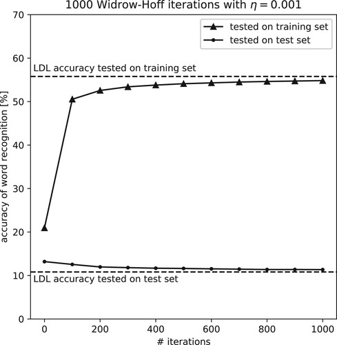
With respect to the test data, we observe the same pattern that characterises model performance on the full data: the incremental learning curves monotonically tend toward the end-state accuracy predicted by LDL. However, whereas with more iterations over the data, accuracy on the training set increases, accuracy on the test set slightly decreases. With more reiterations over the same input, unsurprisingly, the model tunes better and better into seen data at the cost of the unseen data. The network handles this trade-off by gaining more than 35% points in accuracy on the training set while losing less than 2% points on the test set. The discrepancy between performance on the training data and performance on the test data is, however, substantial and indicates the model is largely overfitting the data. An important motivation for the development of LDL-AURIS is to reduce the amount of overfitting.

4.3. Discussion

The four simulation experiments all show that there is no sweet spot for incremental learning, no matter whether accuracy is evaluated on the training or the test data. The endstate is the theoretical asymptote for learning when the number of epochs n through the training data goes to infinity. Our simulations also show that the Widrow-Hoff and Rescorla-Wagner learning rules produce identical results, as expected given the mathematics of these learning rules. Furthermore, our simulations clarify that model performance, irrespective of the estimation method, critically depends on the orthogonality of the semantic vectors. In Section 6, we return to this issue and we will present a way in which similarity (required for empirical linguistic reasons) and orthogonality (required for modelling) can be properly balanced. Finally, comparison of model performance on training data and test data shows that the model is overfitting the data. The next section starts addressing this problem by attending to the question of whether the features extracted from the auditory input can be further improved.

5. Learning with enhanced auditory features

Thus far, we have used the discrete FBS acoustic features proposed by Arnold et al. (2017). These features log patterns of change in energy over time at 21 frequency bands defined on the mel scale, a standard perceptual scale for pitch. These patterns of change are extracted for stretches of speech bounded by minima in the smoothed Hilbert envelope of the speech signal's amplitude (henceforth, chunks), and summarised using a pre-defined set of descriptive statistics.¹¹ The number of different FBS features for a word is a multiple of 21 and the total number of features typically ranges between 21 and 84, depending on the number of chunks.

The FBS algorithm is inspired by the properties and functions of the cochlea, and the basilar membrane in particular. The FBS algorithm decomposes the incoming continuous signal in the time domain into a sum of simple harmonics through a Fast Fourier Transform, similar to the basilar membrane's response to a complex sound with multiple excited regions corresponding to the sound's constituent frequencies, which is enabled by its tonotopic organisation. Furthermore, power values present at different frequencies are summed over a series of filters obtained according to the MEL formula presented in Fant (1973), similar to the cochlea's separation of energy in the input signal by a series of overlapping auditory critical filter banks that jointly are responsible for the nonlinear relationship between pitch perception and frequency. In addition, the energy values are then log-transformed, similar to the logarithmic relationship between loudness perception and intensity. Finally, the algorithm summarises change patterns over time in the energy values at different frequency bands by means of discrete features. An FBS feature extracted from the acoustic input is assumed to correspond to, at a functional level, a cell assembly that is sensitive to a particular pattern of change picked up at the basilar membrane and transferred in the ascending auditory pathway to the auditory cortex.

This approach to signal processing differs from standard approaches, in that the focus is on horizontal slices of the spectrogram, corresponding to different frequency bands on the basilar membrane, instead of the vertical slices in the spectrogram that correspond to phones. Although initial results obtained with this approach are promising (see Arnold et al., 2017; Shafaei-Bajestan & Baayen, 2018, for detailed discussion), one problem with FBS features is that their temporal resolution is restricted to time intervals that are of the order of magnitude of the time between minima in the Hilbert envelope, which correspond roughly to syllable-like units. As a consequence, the model has insufficient temporal granularity to be able to model cohort effects. Furthermore, the discretisation of patterns of change in the frequency bands, necessitated by the use of the Rescorla-Wagner learning rule within the framework of NDL, may come with a loss of precision (see Nenadić, 2020, for a critical discussion of FBS features), and may also underlie the overfitting observed in the preceding section. We therefore investigated whether, within the framework of LDL, this approach can be enhanced. In what follows, we define new features, Continuous Frequency Band Summaries features, and we will show that they have better performance than their discrete counterparts.

5.1. Method

Pseudo-code for C-FBS extraction is given by Algorithm 1 (displayed below), which takes the audio file of a word as input, resamples that using the resample function from the Python package librosa,¹² and returns a feature vector for the word by concatenation of feature vectors for word's chunks.¹³ To assemble a feature vector for a chunk, Algorithm 1 finds the chunking boundaries defined by extrema (minima or maxima) in the Hilbert envelope using Algorithm 2 and calls Algorithms 3 and 4 on each chunk.¹⁴ Algorithm 3⁣⁣⁣⁣⁣⁣⁣ performs a spectral analysis on a chunk and returns the logarithm of energies at MEL-scaled frequency bands using the logfbank function from the Python package python_speech_features.¹⁵ Algorithm 4⁣⁣⁣⁣⁣⁣⁣ summarises the spectrogram of a chunk and returns a feature vector for the chunk.

Summarisation of a chunk's energy information over time can be attempted in various ways. In the present implementation, from the sequence of log-energy values at a particular frequency band and a particular chunk, we extract (1) frequency band number, (2) an order-preserving random sample of length 20, and (3) correlation coefficients of the values at the current frequency band with those of the following bands. In this way, the correlational structure between the frequency bands of a chunk is made available for learning. For chunks shorter than 100 ms, which will not have 20 energy values to sample from (since the FFT window size is 5 ms), zeros are added to the end of the list of the energy values to increase the length to 20. This procedure results in 651-dimensional vectors of real numbers for each chunk.

All feature vectors for words obtained by Algorithm 1 are then padded with trailing zeros to match the length of the feature vector for the word with the largest number of chunks in the dataset. For the current dataset, zero-padded feature vectors have a dimensionality of 6510 and average vector sparsity of 0.8 ($\mathrm{SD}=0.01$).

The C-FBS algorithm, as employed in the present study, identifies chunk boundaries in a word at the maxima of the signal's envelope. The top and middle panels in Figure 11 (see page 73, where it is discussed in more detail) present the chunking boundaries for the audio signal of the word captain in the waveform and in the power spectrum, respectively. The Python implementation of the algorithm, which is also available in the package pyLDLauris, allows the user to fine-tune the chunking criteria. For a visual summary of the FBS and the C-FBS algorithms and some examples for the neighbourhood structure of C-FBS feature vectors, see Appendix C.

The audio tokens in our dataset are, on average, split into 2.23 chunks ($N=131,372$, $\mathrm{SD}=1.07$, range: 1–10) by the C-FBS algorithm. There is a strong positive correlation between the duration of words and the number of chunks detected by the C-FBS algorithm, $r(131,372)=0.85$, p<0.001. The average chunk duration is 114 ms ($N=292,776$, $\mathrm{SD}=55$, range: 10–561).

The FBS algorithm, on the other hand, cannot extract features for audio tokens that are shorter than 50 ms, a condition that is true for 4011 audio tokens in the dataset. Setting these short occurrences aside, the audio tokens for which there is a valid FBS representation are, on average, split into 1.37 chunks ($N=127,361$, $\mathrm{SD}=0.68$, range: 1–8). The average FBS chunk duration is 191 ms ($N=174,289$, $\mathrm{SD}=95$, range: 35–820).

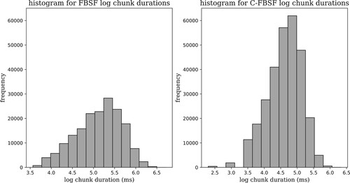
Figure 6 illustrates and compares the distribution of chunk duration by the FBS and C-FBS chunking procedures. Both distributions are approximately log-normal. As the C-FBS algorithm implements more fine-grained smoothing of the Hilbert envelope, it is able to detect more local extrema and produces more and shorter chunks. See Appendix C for minor differences between the FBS and the C-FBS chunking algorithms.

Figure 6. Distribution of chunk durations. Chunk duration follows lognormal distributions in FBS (left panel) and C-FBS (right panel). C-FBS produces more and shorter chunks compared to FBS. Logarithms are to the base of the mathematical constant e.

Table

Algorithm 1 Steps for C-FBS feature extraction
function GETCFBS(word)
wav, sr ← read the word's wave data and sampling rate from audio file word
if sr 6 ≠ 16,000 then resample wav to 16,000
end if
chunks cs ← GETCHUNKS(wav)
word's C-FBS vector wv ?empty vector
for all chunk ∈ cs do
chunk's log MEL energies lme ← GETLOGMELENERGIES(chunk)
chunk's vector v ← GETSUMMARY(lme)
append v to wv
end for
return wv
end function

Table

Algorithm 2 Steps for chunking a stretch of audio
function GETCHUNKS(wav)
analytic signal a ← Hilbert transform of wav
envelope e ← modulus of the complex-valued a
window w ← a boxcar window
smoothed window se ← the convolution of e and w
indices i ← arguments of the maxima for e
chunks c ← segments of wav split by i
return c
end function

Table

Algorithm 3 Steps for spectral analysis of a stretch of audio
function GETLOGMELENERGIES(wav)
STFT ← Short-time Fourier transform of wav using non-overlapping 5ms
Hamming windows and an FFT size of 512
power spectrum ps ← modulus of the complex-valued STFT, squared,
divided by the FFT size
filterbank fb ← 21 auditory critical bands computed based on the MEL formula
of O'Shaughnessy (1987)
MEL power spectrum mps ← apply fb to ps
MEL filterbank energies me ← sum mps for each filter in fb
replace zeros in me with Î = 2.22 ´ 10-16
log MEL energies lme ← loge(me)
return lme
end function

Table

Algorithm 4 Steps for summarising the changes in spectral information into a vector
function GETSUMMARY(lme)
v ← empty vector
for integer i = 1 ® 21 do
append i to v
if length(lme[i])= 20 then
append an order-preserving random sample of length 20 from lme[i] to v
else
zero-pad lme[i] to length 20 and append it to v
end if
for integer j = i + 1 ® 21 do
append correlation between lme[i] and lme[j] to v
end for
end for
return v
end function

We built two models, one using the FBS features of Arnold et al. (2017), the other using the new C-FBS features. Word meanings were represented by means of semantic vectors from the vector space extracted from the TASA corpus with 23,561 word types and morphological functions constructed by Baayen et al. (2019). Henceforth, we denote this space as TASA2.¹⁶ Vectors from TASA2 have dimensionality 4609. TASA2 contains vectors for 4377 of the total number of 4741 word types in the dataset.

5.2. Results

In order to evaluate the accuracy of the C-FBS features, we evaluated recognition accuracy both on the training data itself, and on held-out data using cross-validation. By comparing the accuracy values, we gain further insight into the extent to which models are overfitting the training data. Table 3 presents accuracy in percentage correct for LDL in recognising word tokens of the dataset for which a TASA2 vector is available ($N=123,719$). When LDL is provided with the sparse binary vectors of FBS features, it learns the training data well (accuracy 38.9%), but accuracy under cross-validation plummets to 6.9%, a clear warning that the model is overfitting. When LDL is supplied with C-FBS features, its performance on the training data is worse, compared to the original features, at 16.2%, but performance under cross-validation reduces to only 11.3%, nearly double the performance of the original features, and substantially outperforming the deep learning network tested by Shafaei-Bajestan and Baayen (2018). Results are similar, but slightly inferior, when maxima are replaced by minima in the C-FBS chunking algorithm.

Table 3. Comparison of the performance of LDL using FBS and C-FBS (accuracy of correct word recognition [%]).

Feature extraction	Training accuracy^a	Testing accuracy^b
FBS	38.9	6.9
C-FBS	16.2	11.3

^a Recognition accuracy on training data.^bMean recognition accuracy on test data over 10 cross-validation folds.

What do the new acoustic features represent, and how should they be interpreted? Questions such as these are not straightforward to answer for the discrete FBS features. Since the new C-FBS features are continuous rather than discrete, some insight into what they represent can be obtained relatively straightforwardly by means of clustering methods. Following Baayen et al. (2018), we reasoned that if our acoustic features are understood as the functional equivalent of cell ensembles monitoring for patterns of change in cochlear frequency bands, then the question arises of how such ensembles might be organised in a two-dimensional plane, where this plane is a very rough approximation of some area of the cortex. Given that some topographical clustering of phones has been observed in medical studies (see Cibelli et al., 2015, and references cited there), one may expect phone-like clustering when C-FBS features, which are high-dimensional vectors, are projected onto a two-dimensional space. We used the t-SNE dimensionality reduction algorithm (van der Maaten & Hinton, 2008) as implemented in the scikit-learn Python library (Pedregosa et al., 2011) to visualise the form space in 2D. Essentially, t-SNE is a non-linear technique that is particularly well suited for the visualisation of high-dimensional data and that is often used for interpreting patterns of activation in deep learning models.

To obtain a two-dimensional representation of the C-FBS features, we proceeded as follows. First, we extracted a 651-dimensional C-FBS feature vector for all chunks. Secondly, we computed the list of phones present in a chunk by aligning the phone boundaries and the chunk boundaries. If a phone is split between two chunks, the phone is considered to be contained in the chunk with the longer stretch of the phone's audio signal. This resulted in a matrix with for each phone token a 651-dimensional row vector of the C-FBS feature for the chunk in which that phone was present. This matrix with phone tokens was then first subjected to a Principal Components Analysis, resulting in an orthogonalised space that in a final step was presented as input for the t-SNE.

In what follows, we zoomed in on those chunks that contained one of the phones [b, p, d, t, ɑ, e, i] and that did not fully contain any other phones. Table 4 reports the frequency of occurrence for all pertinent chunk-phone combinations. Figure 7 presents the locations in the t-SNE topographic map of the chunk-phone combinations for [b] and [d] (left panel) and [p] and [t] (right panel). For both pairs of consonants, we see some clustering with fractal-like properties. The centre-most clusters of points predominantly represent [d] and [t] respectively, with a subcluster of [b] and [p] in their respective peripheries. This pattern repeats itself in the smaller satellite clusters. Comparing the two plots, it is noteworthy that [d] (blue) and [t] (purple) show highly similar clusters, perhaps unsurprisingly given that they only differ in voice onset time. The isomorphism between [b] and [p] is less clear. This, however, may be due to the substantially smaller number of data points present for these phones. Overall, the similarity of the two plots shows that the labial-alveolar contrast is in like manner captured for both [b]–[d] and [p]–[t]. A similar fractal-like structure emerges for the vowels [ɑ, e, i], as shown in Figure 8, with recurring leaky separation of [i] from [e] and [ɑ], and some further separation within the [e] and [ɑ] clusters. The apparent difference between consonants in Figure 7 and vowels in Figure 8 has not been hand-crafted into the features, e.g. by representing the input in terms of binary vectors over phonemic features; instead, it emerges from the structure of the C-FBS feature space.

Figure 7. Topographic map of stop consonants visualised by t-SNE clustering.

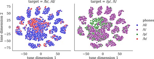
Figure 8. Topographic map of peripheral vowels visualised by t-SNE clustering.

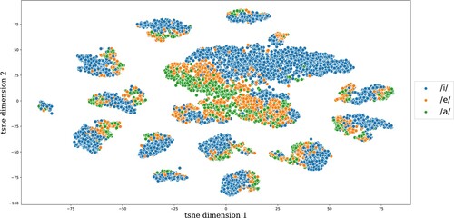
Table 4. Frequencies for chunks comprising one phone used in t-SNE analysis.

Phone in chunk	Chunk frequency
[b]	2588
[p]	1985
[d]	6603
[t]	11,633
[ɑ]	2114
[e]	2600
[i]	6866

5.3. Discussion

The FBS features developed by Arnold et al. (2017) cover stretches of speech that are syllable-like. The temporal granularity of these features is too coarse to allow modelling of cohort effects in auditory word recognition. A comparison of the distribution of chunk duration in FBS features with the newly developed C-FBS features revealed that the C-FBS features cover shorter stretches of speech. We return to the question whether this provides us with sufficient granularity in time to predict cohort effects using C-FBS features in Section 7.2.

From the LDL simulations using FBS and C-FBS algorithms, we conclude that the features from C-FBS substantially attenuate the over-fitting problem that characterises the LDL model when using the FBS features. For generalisation, working with real-valued acoustic features instead of discrete summary features offers a clear performance improvement. We therefore use the C-FBS features in the simulation experiments presented in Section 7.

From the t-SNE analysis of C-FBS features we can conclude that, even though these features slice the spectrogram horizontally, along cochlear frequency bands instead of vertically, phone by phone, they nevertheless preserve substantial information about phone classes. At the same time, the overlap between the consonant maps and the vowel map indicates that phones need not be uniquely represented in the map, but will often share a position in the map with other phones. This makes perfect sense from a phonetic perspective, as co-articulation is ubiquitous. For the present phones, for instance, place of articulation of the stops is signalled by the formant transitions in the vowels they co-occur with. Importantly, even though in our model the theoretical construct of the phoneme does not play a role, the C-FBS features are sufficiently rich to capture similarities and dissimilarities between phonemes. These similarities, in turn, co-determine the mapping from form onto meaning. Thus, in our approach, phones are not emergent on some hidden layer of a deep learning network, but rather are implicit in the input vectors.

In the next section, we consider whether the representation of meaning in NDL and LDL can be enhanced further.

6. Learning with enhanced semantic vectors

In Section 4, we observed that semantic vectors derived from the TASA corpus underperformed considerably compared to either one-hot encoded semantic vectors or near-orthogonal vectors of random numbers. This observation suggests that ideally semantic vectors should strike a balance between being well discriminable (close to orthogonal) while at the same time reflecting the semantic similarities that native speakers perceive when judging word pairs (see, e.g. the MEN dataset compiled by Bruni et al., 2014).

Would semantic vectors as constructed by means of machine learning methods in the computational linguistics community, such as word2vec (Mikolov et al., 2013),¹⁷ provide a proper balance? Although these vectors are very good predictors of human-perceived semantic similarity ($r(1176)=0.76$, p<0.001 for the set of words shared between the MEN and our speech dataset), they are trained on approximately 100 billion words from the Google News^TM data. This volume is far more than anyone will ever encounter in their lifetime. Estimates vary among authors, but we can expect that language users' exposure amounts to roughly 9 to 25 million words per year, so at best, the training set is equivalent to 4000 years of a single human's experience; see Uhrig (2018b, pp. 280–281) for a brief discussion and further references. Thus, from a cognitive perspective, such vectors are unrealistic, as they are tuned to vastly more knowledge (including the full Wikipedia) and linguistic experience than anybody can ever assemble in a lifetime. Thus, while training with massive data may give rise to semantic vectors that are distinct enough to be both discriminable and faithful to semantic similarity, we decided against them for reasons of cognitive implausibility.

In what follows, we consider whether TASA2 semantic vectors trained on “only” 10 million words taken from the TASA corpus can be enhanced by adding some small amount of random noise. Technically, the idea is that by adding some noise, the semantic vectors become more discriminable, and therefore can be better predicted from the acoustic feature vectors. In other words, addition of noise is motivated here first of all as a data augmentation technique, widely used in machine learning to avoid overfitting (see Shorten & Khoshgoftaar, 2019, for noise injection in image processing and D. Zhang & Yang, 2018, for noise perturbation of word embeddings.) Adding noise also implements, however crudely, that words' meanings are richer, in word-specific ways, than can be captured from textual data. A growing body of literature shows that perceptually grounded word embeddings outperform those created from word co-occurrence information alone (see Shahmohammadi et al., 2021, for state-of-the-art visually grounded word embeddings).

6.1. Method

We contrasted learning with four semantic spaces. The first two are the semantic spaces TASA1 and TASA2 that we introduced in previous sections. Two additional vector spaces were built by element-wise addition of 4377 noise vectors with 4609 dimensions to the semantic vectors of TASA2. Noise vectors were sampled from a Gaussian distribution with $\mu =0$ and standard deviations 0.001 (henceforth, small amount of noise) and 1.0 (large amount of noise) respectively.

We assessed the degree of orthogonality of the resulting four semantic spaces with two evaluation metrics, the average correlation and the average variance. We computed the average correlation for a semantic space by taking the average of the Pearson r correlation coefficients for all pairs of semantic vectors in that space. The lower the average correlation, the closer to orthogonal the set of vectors in the space is. The average variance for a semantic space is the average over all semantic vectors in the space of the variance of these vectors. A higher average variance also implies that the set of vectors in the space is closer to orthogonal.

The data to which we applied these measures comprised all 4377 word types for which semantic vectors are available in TASA and which appear in our speech dataset. LDL models were trained to discriminate distributional features of the different TASA semantic spaces using FBS features. Model accuracy was evaluated on the training set. The extent to which a semantic space captures the semantic structure of the lexical representations was examined on the MEN database (Bruni et al., 2014) that provides for 3000 word pairs crowdsourced ratings of semantic similarity. For 1176 word pairs, semantic vectors are available in all semantic spaces for both words. For this subset of words, we evaluated to what extent our semantic vectors matched human-perceived similarity. The subset is properly representative of all word pairs in MEN. A Wilcoxon rank-sum test failed to reject the null hypothesis that the distribution of ratings of word pairs in the subset ($\mathrm{Mdn}=26.5$) and the distribution of ratings of all pairs ($\mathrm{Mdn}=26$) are different ($W=1,374,230$, p=0.14).

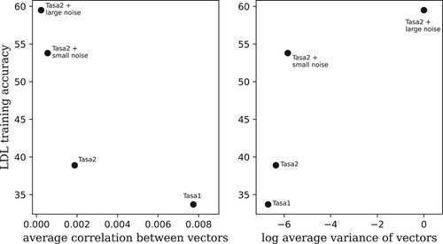
6.2. Results

Figure 9 plots the training accuracy of the LDL model against the average correlation of the semantic space in the left panel, and against the average variance of the semantic vectors in the right panel. LDL training accuracy increases with lower average correlation and higher average variance, as expected. TASA1 vectors obtained from a smaller subset of TASA have the least discriminated features and are not well discriminated by LDL. More data in the training of TASA2 compared to the training of TASA1, resulted in a vector space with more distinct vectors, thereby facilitating learning. Adding a tiny amount of noise boosted accuracy substantially. Increasing the standard deviation of the noise a thousandfold offered only a minor further improvement.

Figure 9. Orthogonality measures, average correlation (left panel) and average variance (right panel), as predictors of LDL accuracy evaluated on the training data.

Table 5 lists the Pearson's coefficients for the correlation between the MEN ratings for pairs of words and the semantic similarities of the corresponding two semantic vectors from our semantic spaces. The gain in capturing semantic similarities of words achieved in TASA2 compared to TASA1 is likely due to a larger subset being used when training the TASA2 space. Addition of a tiny amount of Gaussian noise brought down the correlation somewhat while at the same time, as demonstrated above, affording a substantial boost in prediction accuracy. Addition of substantial noise almost completely removed lexical similarity structure from the vectors, while offering only a modest additional accuracy gain.

Table 5. Similarity structure of semantic spaces.

Vector space	r	p-value
TASA1	0.24	<0.0001
TASA2	0.59	<0.0001
TASA2 plus small amount of noise	0.47	<0.0001
TASA2 plus large amount of noise	0.02	0.4946

Note: Pearson's correlation coefficient r and p-value for the strength of relationship between the similarity ratings provided by the MEN dataset and the similarity scores calculated from the vectors of each semantic space. Degrees of freedom is 1174 for all tests.

6.3. Discussion

Addition of a tiny amount of noise to the TASA2 vectors boosted accuracy, evaluated on the training data, by about 15% points to 53.8%. When we in addition consider accuracy for these vectors under 10-fold cross-validation, we also observe an improvement from 6.9% to 11.1%. Interestingly, LDL performance with word2vec vectors was not as good (52.6% accuracy on training data, but only 8.5% averaged on 10 folds of test data). We therefore use the TASA2 vector space with a tiny amount of noise added in our final simulations presented in the next section, which introduces our best and definitive model. The addition of Gaussian noise reduces skewness and kurtosis of the distributions of semantic vectors, reducing outlier effects, and thus facilitating learning (see Appendix D for further details).

7. Putting it all together

Our final simulation study combines the insights of the preceding sections to define an improved discriminative model for auditory word recognition that we have named LDL-AURIS. This model makes use of C-FBS features to represent words' auditory forms, it uses empirical, as opposed to simulated random, semantic vectors derived from TASA with a small amount of noise added, and it estimates network weights using multivariate multiple regression.

In what follows, we report on the model's performance, focussing on two main questions. First, the accuracy of the new model is of interest, both for the training data on the one hand, and under 10-fold cross-validation on the other hand. Second, does the better temporal granularity of the C-FBS features compared to the FBS features, make it possible to now predict the cohort effects that are known to characterise human auditory word comprehension?

When assessing model performance, it should be kept in mind that the audio from which C-FBS features were derived is far from perfect: the automatic alignment has an error rate of around 12% (Uhrig, 2021), and uses the closed captions which themselves may not correspond to what speakers exactly said.

7.1. Accuracy

LDL accuracy was 25% on training data and average LDL accuracy under 10-fold cross-validation was 16%. Compared to the model presented in Baayen et al. (2019), the model showed an 8% point decrease in training accuracy but an 8% point increase in test accuracy, considerably reducing the extent of the over-fitting problem. When we consider the number of target semantic vectors among the top 5 and top 10 words showing the strongest correlations with the predicted semantic vector, accuracy increases to 57% and 75% on training data and to 37% and 50% on test data. Thus, model accuracy comes close to the lower bound of the range of human recognition accuracy documented for single word recognition tasks (Arnold et al., 2017; Pickett & Pollack, 1963; Pollack & Pickett, 1963). The performance of our model contrasts favourably with the recognition rate of Mozilla Deep Speech, which was roughly 10% points lower (Shafaei-Bajestan & Baayen, 2018). This is not to say that deep learning methods applied to exactly the same data as we are investigating here cannot reach the same level, or even a better level, of accuracy, but rather that, given the complexity of the task and the simplicity of the model, performance of LDL-AURIS is surprisingly good. In this respect, it is noteworthy that the data on which we train and test the model comes from many different speakers from a wide range of backgrounds, and that we did not apply any speaker normalisation.

Accuracy numbers reported throughout the paper show that the observed improvement in the performance of the final model is due to both the enhancement of the feature space in Section 5 and the enhancement of the semantic space in Section 6. Model performance on unseen data increased by 5% points when features were upgraded, by 4% points when semantic vectors were refined, and by 9% points when both were altered. The extent of overfitting to training data, gauged by the observed difference between model performance on the training and test sets, decreased by 34% points with modification of features alone, increased by 11% points with modification of semantic vectors alone, and decreased by 34% points with simultaneous modification of features and semantic vectors. In other words, the benefits of all changes to the model are perfectly additive.

It is known for human auditory word recognition that higher-frequency words are recognised more accurately, as well as more quickly (see, e.g. Baayen et al., 2007; Connine et al., 1993; Seidenberg & McClelland, 1989). We used a generalised additive model (henceforth, gam) with a logistic link function, using the mgcv package for R (Wood, 2017), to predict whether LDL-AURIS correctly identified a word token, using log word frequency and log duration as predictors.¹⁸ Partial effects are shown in Figure 10, and Table 6 provides the summary for the gam. Longer words are recognised more often by LDL-AURIS, and the same holds for more frequent words. The advantage for longer words, given the negative correlation of frequency and length, shows that LDL-AURIS does not depend on only frequent use, but is also properly sensitive to the amount of information in the speech signal. The rightmost panel of Figure 10 shows the frequency effect predicted for auditory lexical decision. Here, we assume that the time required for making a lexical decision is inversely proportional to the probability predicted by the gam that LDL-AURIS correctly understands the word. The nonlinear effect of frequency, with a levelling off for higher frequencies, resembles the kind of nonlinear effect typically observed in reaction time studies of reading (see, e.g. Baayen, 2005; Ramscar et al., 2014). A similar pattern also characterises the auditory lexical decision times in the MALD database (Tucker et al., 2019) (model not shown). Thus, qualitatively, the model provides a good approximation of the shape of the word frequency effect.

Figure 10. Partial effects of log word duration (left) and log word frequency (center) on LDL-AURIS recognition accuracy according to a logistic generalised additive model. The right panel presents the reciprocal of the probability of identification as a function of frequency, the hypothesis being that words with a greater probability of identification can be responded to more quickly in a lexical decision task.

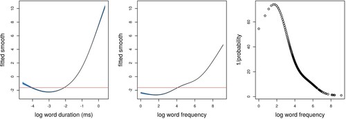
Table 6. Summary of the gam.

A. parametric coefficients	Estimate	Std. Error	t-value	p-value
(Intercept)	−1.6120	0.0100	−161.2772	<0.0001
B. smooth terms	edf	Ref.df	F-value	p-value
s(logdur)	3.9816	3.9998	15,377.9701	<0.0001
s(logfreq)	3.9902	3.9999	20,071.5283	<0.0001

7.2. Cohort effects

We observed in Section 5 that the temporal granularity of the C-FBS features is more fine-grained than that of the FBS features. To clarify whether this provides our new model with sufficient granularity in time to predict cohort effects, we constructed words' audio vectors incrementally. For a given word with C-FBS vector $\mathit{c}$, and for each of its temporally ordered successive chunks 1 through k, we first constructed a feature vector ${\mathit{c}}_i$ that contained the C-FBS features for the ith chunk, and zeroes elsewhere. Importantly, $\sum _{i=1}^k{\mathit{c}}_i=\mathit{c}$. We then calculated, for each of the successive chunks at “chunk time” t, the cumulative feature vector ${\mathit{c}}_t=\sum _{i=1}^t{\mathit{c}}_i$. Finally, for each cumulative form vector ${\mathit{c}}_t$, we calculated the corresponding semantic vector ${\hat{\mathit{s}}}_t=\mathit{F}{\mathit{c}}_t$. Note that ${\hat{\mathit{s}}}_k=\hat{\mathit{s}}$. In other words, instead of carrying out the matrix multiplication $\mathit{F}\mathit{c}$ all at once, this multiplication is carried out staggered over time. Because at each successive chunk a word's semantic vector is updated, we obtain a time-ordered sequence of semantic vectors that can be conceptualised as a path or trajectory in semantic space. This conceptualisation of understanding over time as creating a path in lexical-conceptual space is indebted to Elman (2009).

The lower panel of Figure 11 illustrates the time course of lexical processing for the target word captain, comparing the correlation of the predicted semantic vector with that of captain for three input words, cap, capital, and captain. There are 8, 22, and 7 audio tokens respectively for these three words in our dataset. From this list of tokens, we randomly selected one audio token for each word, with as constraint that, for plotting reasons, the number of chunks in the competitors does not exceed the number of chunks in the target word. The upper panel of Figure 11 presents the audio signal of the selected token for captain, together with its Hilbert envelope. The red vertical lines highlight where the Hilbert envelope of the token captain reaches a local maximum. The selected audio tokens of cap and capital have their local maxima at 0.17 s and 0.14 s, and have a total duration of 0.37 s and 0.41 s, respectively. The centre panel presents the MEL spectrogram corresponding to the audio token of captain shown in the top panel, with on the vertical axis the 21 auditory filter banks inspired by the tonotopy of the basilar membrane in the cochlea.

Figure 11. Time course of lexical access for the target word captain. Top panel: the waveform for a token of the word captain in dark gray, and the Hilbert amplitude envelope of the signal in orange. The red vertical lines indicate chunk boundaries, located at the arguments of local maxima of the Hilbert envelope at 0.18 s and 0.36 s. The dashed black vertical line at 0.4 s indicates the end of word boundary. Mid panel: the corresponding log MEL spectrogram split at 21 auditory filter banks shown on the y-axis. Lower panel: semantic similarity, as measured by Pearson's correlation coefficient r, to the target word as a function of time, for the target word captain and two competitors cap and capital. For each word, similarity is calculated as many times as the word has chunks, with each measurement being made between the target's semantic vector and the semantic vector predicted from the partial cue vector available at that point in time. The dashed lines are the linear interpolants between pairs of measured data points. The colour-coded transcripts at the bottom show the phonemes present in the chunks for the three words. Click on the words below or scan QR codes to listen to the audio.*See page 38, where this figure was first referenced.

   

   

*The links use the Distributed Little Red Hen Lab's permalink infrastructure, introduced in Uhrig (2020).

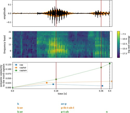
With respect to the time course of lexical processing, in the beginning, at t=0, no auditory information is present, and the word's meaning is located at the origin of the semantic space. On the presentation of the first chunk, the model has detected that all three candidates approximate the target semantic vector to some extent, with captain already taking the lead. Since the word cap covers a longer stretch of the signal for [æ] in its second chunk, it is not a strong competitor at the first chunk. The average correlation value for all the 55 tokens of 9 types that start with [kæp] is 0.022 at the end of their first chunks. All seven occurrences of captain are correlated with the target vector well above the mean at the end of the first chunk (M=0.041, $\mathrm{SD}=0.009$). By the end of chunk two, cap and capital in decline and lose out further to captain. The arrival of [n] in the final chunk pushes the predicted semantic vector of captain even closer to the target vector.

Instead of aligning words by time in ms, we can align words by chunks. This enables straightforward calculation of 95% confidence intervals around the sample means of semantic similarities to the target word over time computed across different audio renditions of each word type.

The top left panel of Figure 12 shows the same trend observed in the bottom panel of Figure 11, now not for one randomly-chosen occurrence for each of the word types, but instead taking into account all occurrences of captain with 3 chunks (4 tokens), cap with 2 chunks (8 tokens), and capital with 4 chunks (9 tokens). After the presentation of the first chunk, error bars are still overlapping. After the presentation of the second chunk, the semantic similarities to the target word predicted from audio tokens of captain are well-separated from the similarities of the competitors.

Figure 12. Evolving proximity to targeted semantic vectors as a function of number of chunks encountered. Horizontal axes represent time t discretised into C-FBS chunks. Vertical axes present the average time specific semantic similarity of predicted semantic vectors ${\hat{\mathit{s}}}_t$ with the targeted semantic vector across different audio tokens of competitor word types. Vertical lines denote 95% confidence intervals. Coloured lines connect data points belonging to the same word type. In the top left panel, the target word is captain and the competitors, cap, capital, and captain, were selected by hand. In all other panels, the competitors are generated from the canonical pronunciations available in the CELEX database.

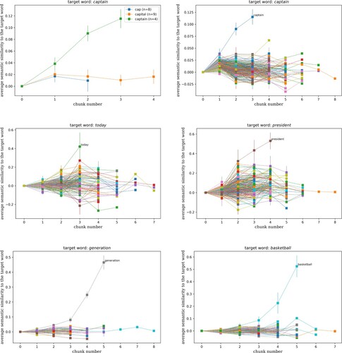
The top right panel of Figure 12 is computed in the same way as the top left panel, but extends the set of competitors in the cohort for captain from cap, capital, and captain to all of the words in the database that partially match the beginning of the word captain according to canonical pronunciations given by CELEX (Baayen et al., 1995). This includes all of the 439 word types in the database that start with [k]. Of these, 49 start with [kæ], 8 start with [kæp], 2 start with [kæptɪ] and 1 starts with [kæptɪn]. The words types have token frequencies from 1 to 196 (M=6.2, $\mathrm{SD}=16.2$) and are split into 1 to 8 chunks (M=3.3, $\mathrm{SD}=1.2$). As before, we find that although after the first chunk the model is already zooming in on its gold standard semantic vector, there is still strong competition. After the second chunk has become available, all other competitors are left behind.

The remaining panels of Figure 12 present the time course of lexical processing for five target words: today with 229 competitor types, president with 356 competitor types, generation with 66 competitor types, and basketball with 293 competitor types, with the cohorts of competitors determined by the CELEX pronunciations. In all of the example plots, the target audio tokens end up closest to the target semantic vector and wins the competition. For a total of 342 target words for which we carried out a cohort analysis, the target word was the correct winner in 91% of the cases. There were 32 target words who lost to a competitor. Of these, 88% still were among the top 10. Many of the errors made by the model are reasonable. Some of the errors are homophonous words. For example, the competitor inn is the winner for the target word in. Generally, defeated target words have fewer chunks and are embedded in a greater number of carrier words, compared to the winning target words. The target word see, for example, is the runner-up after the competitor seas. This short word is acoustically embedded in 20 carrier words, leading to heavy competition (X. Zhang & Samuel, 2015). Here, it should be kept in mind that especially for very short words, the accuracy of the forced aligner used to find word boundaries in the acoustic signal is lowest.

In classical models of lexical processing, in which words' forms are accessed in parallel, the present time course plot would be understood as demonstrating multiple access and multiple simultaneous assessment unfolding efficiently in real time. In fact, Marslen-Wilson (1987) argued that a model of spoken word recognition should meet three functional requirements. First, models should properly reflect “multiple access”. Our model can be interpreted to indicate that all three words are accessed simultaneously, forming a class of potential word candidates compatible with the sensory input. Second, models should reflect “multiple assessment” of word candidates. Our model appears to meet this requirement as by the end of the first chunk, where multiple candidates are compatible with the input, the system already ranks candidates. Third, models should accommodate multiple access and assessment in real time. Our model also satisfies this requirement: within about 200 ms from word-onset, the target word is beginning to be recognised, and as more chunks become available, candidates' rankings are recalibrated.

However, the general conceptualisation underlying our model differs from that of Marslen-Wilson (1987). Our model construes understanding as it develops over time as speech comes in as a path through lexical space (cf. Elman, 2009). There are no discrete processing stages nor a final state in which a word has been accessed, but rather a gradual process of uncertainty reduction (see also Baayen et al., 2015; Ramscar, 2013; Ramscar et al., 2013) that, importantly, does not need to resolve into a winner-take-all state of absolute certainty. Thus, even though the conceptualisation of the process of “lexical access” is different from that of TRACE or SHORTLIST, our model does show the kind of temporal dynamics that has been an important explanandum for classical models.

8. General discussion

The computational model for auditory word recognition laid out in this study builds on an earlier model proposed by Arnold et al. (2017), enhancing it in several ways. First, real-valued feature vectors extracted from the speech signal replaced discrete binary vectors, while maintaining the important insight that cochlear frequency bands can inform feature engineering for cognitive modelling. Second, discrete binary vectors with one-hot encoding for words' meanings were replaced by real-valued semantic vectors. By adding a small amount of noise to vectors derived from a relatively small corpus (TASA) using distributional semantics, semantic vectors were obtained that are sufficiently discriminable while respecting semantic similarities between words. Third, instead of using incremental learning using the Rescorla-Wagner learning rule, with one pass through the data, we estimated the endstate of learning using the mathematics of multivariate multiple regression, which simulation studies show to offer greater accuracy. In fact, LDL-AURIS can be seen as a statistical model for auditory comprehension, with a fixed algorithm that itself cannot be tweaked, but that can be applied to different datasets, and that will work better, or worse, depending on, first, how exactly form and meaning representations are defined, and second, on the quality, quantity, and nature of the training data (see Heitmeier et al., 2021, for detailed discussion).

Together, these new design features offer the following advantages. First, overfitting on the training data is substantially reduced, whereas prediction for unseen data, evaluated by means of 10-fold cross-validation, improved substantially. The gain in model performance of our best model is exactly the sum of the gains in performance of simpler models implementing once upgrade only.

Second, the new acoustic features provide enhanced temporal granularity, allowing the model to correctly predict cohort-like effects as the speech signal unfolds over time.

Third, the new acoustic features are better interpretable, as shown by projecting form vectors onto a two-dimensional plane with t-SNE. In this plane, phone-like clusters emerge. This shows that even though our acoustic features are based on horizontal slices from the spectrogram (following cochlear frequency band separation) instead of on vertical slices representing phones, information about phones is implicit in our acoustic feature vectors.

The clusters that emerge from the t-SNE projection of acoustic vectors onto a two-dimensional “cortical map” may shed light on the topological clustering observed for phones in the cortex (Cibelli et al., 2015). Whereas at first sight, the neuro-anatomical evidence seems to provide strong evidence that phones, as abstract functional units, are represented in the brain, under our interpretation, such phone clusters emerge from the constraints that come with processing high-dimensional vectors in much lower-dimensional neural tissue. Speculatively, clustering cell assemblies that fire for similar acoustic feature vectors may reduce the metabolic costs of lexical processing, thanks to pooling of functionally equivalent connections.

In this study, we considered monomorphemic words, and derived words with monomorphemic base words, but no inflected variants of these words. However, the general framework within which the present study is conceived, the “discriminative lexicon” as outlined in Baayen et al. (2019), sets up semantic vectors for inflected words by taking the semantic vector of the base word and adding the semantic vectors of the pertinent inflectional functions. Within this framework, the comprehension model of Estonian noun declension presented in Chuang et al. (2019) is reasonably accurate for unseen forms when it is trained on incomplete paradigms (see also Heitmeier et al., 2021). A question for further research is whether LDL networks will remain productive with respect to unseen inflected words when the form vectors using symbolic representations of form (such as triphones) are replaced by real-valued vectors derived from the acoustic signal itself.

Model performance was evaluated on real spontaneous speech, by many different speakers, taken from the NewsScape English Corpus (Uhrig, 2018a). As the automatic alignments in this corpus are not perfect, especially for very short words, the audio data that is the input to our model is not noise-free. Nevertheless, comprehension accuracy under 10-fold cross-validation was at 16%, which is close to the lower bound of human accuracy on the task of recognising auditory words presented in isolation. We note here that this accuracy, which is higher than that obtained by Mozilla Deep Speech evaluated on the same data, is achieved without speaker normalisation.

Our best results are based on the regression approach to estimating the mapping from form to meaning. However, human learning is incremental, and it is therefore important that the weights of the regression model can in principle be learned incrementally with incremental regression using the Widrow-Hoff learning rule. In this study, we have seen that incremental learning requires many passes through the data before it converges to the asymptote provided by standard multivariate multiple regression. This is informative in two ways. First, it clarifies that the endstate of learning is truly conditional on the training data. From the perspective of incremental learning, this implies incremental learning on an infinite number of epochs through the training data. As a consequence, effects of frequency of use are no longer strongly present at the endstate of learning (see Heitmeier et al., 2021, for further details). Second, as human learners never experience the same sequence of learning events time and time again, the endstate of learning is an ideal that is likely to be less idealistic as the amount of training data increases. It is currently an open question how the model will perform on substantially larger amounts of more variegated training data. What is clear is that when LDL-AURIS is applied to small amounts of synthesised speech, or to small amounts of laboratory speech, its performance will be unrealistically high.

Fortunately, the amount of audio offered in the NewsScape corpus is so huge that we can train the model incrementally on thousands of hours of audio, without ever having to repeatedly present a specific acoustic word token twice. An important goal for future research is to clarify how well our new model performs when challenged with such large volumes of speech.

Another important goal for the present research programme is to move from modelling isolated word recognition to the modelling of the understanding of continuous speech, perhaps along the lines of Baayen, Shaoul, et al. (2016). Our model outperforms on isolated word recognition two deep learning models that we have explored (see Arnold et al., 2017; Shafaei-Bajestan & Baayen, 2018, for further details). As isolated word recognition is a task that humans can do with much higher accuracy, it provides a useful, challenging test case for deep learning models of speech recognition. It should be acknowledged, however, that our model is conditional on its – highly restricted – training data, whereas at the same time the deep learning models show impressive performance when it comes to the recognition of continuous speech.

In summary, we have presented a mathematically very simple model for the mapping from acoustics to meaning. Combined with sufficiently rich and sufficiently distinctive high-dimensional representations for form and meaning, this simple model, trained on highly variable and somewhat noisy spontaneous English, already succeeds in predicting several central findings in experimental studies of human auditory comprehension. Thus, it provides further proof of concept that in order for auditory comprehension to be successful, it is not necessary to first extract phonemes from the speech signal. Of all computational models in psycholinguistics, only the Distributed Cohort Model (Gaskell & Marslen-Wilson, 1997) has argued that phonemes are not necessary as mediating units, but their model contains a hidden layer which might have a functionality in the network similar to that of phoneme layers in models such as SHORTLIST-B (Norris & McQueen, 2008). What our simulation studies with LDL-AURIS suggest, by contrast, is that even such hidden layers are not strictly necessary. Actual computations in the brain are much more sophisticated than the simple mappings used by LDL-AURIS. Nevertheless, at the present high level of mathematical abstraction, these mappings can be surprisingly simple.

Acknowledgements

The authors thank the Distributed Little Red Hen Lab, co-directed by Francis Steen and Mark Turner, for making parts of the NewsScape dataset available to us, and two anonymous reviewers for excellent critical discussion.

Disclosure statement

No potential conflict of interest was reported by the author(s).

Data availability statement

The dataset and the Python scripts that support the findings of the final model of this study are openly available in our supplementary materials on “Open Science Framework” at http://doi.org/10.17605/OSF.IO/TDJA2.

Additional information

Funding

This research was funded by the European Research Council under the ERC grant number 742545, Project WIDE, awarded to the last author. The data processing of the NewsScape corpus was funded by the Competence Network for Scientific High Performance Computing in Bavaria to the third author.

Notes

1 Chuang et al. (2020) and Hendrix et al. (2019) show how pseudowords can be processed in models without phones as pivotal units.

2 The term vector is used throughout the paper from a mathematical perspective to refer to a member of a vector space over the set of real numbers, assuming that the axioms of vector spaces are satisfied. For simplicity, one might think of a vector as an ordered list of numbers.

3 For details on how NDL and LDL model the processing of morphologically complex words, see Baayen et al. (2018), Chuang et al. (2019), and Baayen and Smolka (2020).

4 For further details and optimised code for incremental learning, including also the Kalman filter, see Milin et al. (2020).

5 See https://github.com/mozilla/DeepSpeech (last accessed June 26, 2020).

6 See Heitmeier and Baayen (2020) for the importance of working with empirical semantic vectors in computational modelling studies.

7 See http://newsscape.library.ucla.edu/ and http://tvnews.library.ucla.edu/ (last accessed June 26, 2020).

8 See http://lowerquality.com/gentle (last accessed June 26, 2020).

9 A small percentage of the data comprises inflected forms (6%) and compound words (less than 2%) which were not detected by our tagging algorithms.

10 Baayen et al. (2019) constructed a semantic vector space by training an NDL network on the TASA corpus. The network was trained to predict, for all sentences, all the lexomes (words, inflectional functions such as PLURAL, and derivational functions such as AGENT for agents with er) in a sentence from the same lexomes in that sentence. The row vectors of the resulting lexome-to-lexome weights matrix are the obtained semantic vectors, after having the main diagonal of the matrix set to zero and retaining the 4609 columns, out of 12,571, with the highest variances. See Section 2 of that paper for more details and validation of the vectors.

11 The complete set contains the frequency band number, the chunk number, the first, the last, the minimum, the maximum, and the median of the normalised, discretised log MEL energy values.

12 See https://librosa.org/doc/main/index.html (last accessed June 26, 2020).

13 We used a sampling rate of 16,000, a compromise between audio quality and feasibility of C-FBS feature extraction.

14 In our current implementation, minima and maxima are detected on the entire word. This is however only an implementation detail. The detection can also be implemented incrementally in such a way that features become available sequentially in time.

15 See https://python-speech-features.readthedocs.io/en/latest/ (last accessed June 26, 2020).

16 The training procedure for TASA2 was similar to that of TASA1, only with a larger training set of approximately 10 million tokens. Nevertheless, the training set for TASA2 is not a superset of the training set for TASA1.

17 Obtained from https://code.google.com/archive/p/word2vec/ (last accessed June 26, 2020)

18 A model that includes the interaction between length and frequency suffers from substantial concurvity, rendering it uninterpretable. This model is available in the supplementary materials.

References

- Arnold, D., Tomaschek, F., Sering, K., Lopez, F., & Baayen, R. H. (2017). Words from spontaneous conversational speech can be recognized with human-like accuracy by an error-driven learning algorithm that discriminates between meanings straight from smart acoustic features, bypassing the phoneme as recognition unit. PLOS ONE, 12(4), Article ID e0174623. https://doi.org/10.1371/journal.pone.0174623
- Baayen, R. H. (2005). Data mining at the intersection of psychology and linguistics. In A. Cutler (Ed.), Twenty-first century psycholinguistics: Four cornerstones (pp. 69–83). Erlbaum.
- Baayen, R. H., Chuang, Y.-Y., & Blevins, J. P. (2018). Inflectional morphology with linear mappings. The Mental Lexicon, 13(2), 230–268. https://doi.org/10.1075/ml
- Baayen, R. H., Chuang, Y.-Y., Shafaei-Bajestan, E., & Blevins, J. (2019). The discriminative lexicon: A unified computational model for the lexicon and lexical processing in comprehension and production grounded not in (de)composition but in linear discriminative learning. Complexity, 2019, Article ID 4895891. https://doi.org/10.1155/2019/4895891
- Baayen, R. H., Milin, P., Filipović Durdević, D., Hendrix, P., & Marelli, M. (2011). An amorphous model for morphological processing in visual comprehension based on naive discriminative learning. Psychological Review, 118(3), 438–482. https://doi.org/10.1037/a0023851
- Baayen, R. H., Milin, P., & Ramscar, M. (2016). Frequency in lexical processing. Aphasiology, 30(11), 1174–1220. https://doi.org/10.1080/02687038.2016.1147767
- Baayen, R. H., Milin, P., Shaoul, C., Willits, J., & Ramscar, M. (2015). Age of first encounter and age of acquisition norms: What raters do when asked the impossible [Manuscript]. University of Tübingen.
- Baayen, R. H., Piepenbrock, R., & Gulikers, L. (1995). The CELEX lexical database (CD-ROM). Linguistic Data Consortium, University of Pennsylvania.
- Baayen, R. H., Shaoul, C., Willits, J., & Ramscar, M. (2016). Comprehension without segmentation: A proof of concept with naive discriminative learning. Language, Cognition, and Neuroscience, 31(1), 106–128. https://doi.org/10.1080/23273798.2015.1065336
- Baayen, R. H., & Smolka, E. (2020). Modelling morphological priming in German with naive discriminative learning. Frontiers in Communication, Section Language Sciences, 5, Article 17. https://doi.org/10.3389/fcomm.2020.00017
- Baayen, R. H., Wurm, L. H., & Aycock, J. (2007). Lexical dynamics for low-frequency complex words: A regression study across tasks and modalities. The Mental Lexicon, 2(3), 419–463. https://doi.org/10.1075/ml.2.3.06baa
- Bitterman, M. (2000). Cognitive evolution: A psychological perspective. In C. Heyes & L. Huber (Eds.), The evolution of cognition (pp. 61–79). MIT Press.
- Bruni, E., Tran, N.-K., & Baroni, M. (2014). Multimodal distributional semantics. Journal of Artificial Intelligence Research, 49(2014), 1–47. https://doi.org/10.1613/jair.4135
- Butterworth, B., (Eds.). (1983). Language production volume 2: Development, writing and other language processes. Academic Press.
- Chomsky, N., & Halle, M. (1968). The sound pattern of English. Harper & Row.
- Chuang, Y.-Y., Loo, K., Blevins, J. P., & Baayen, R. H. (2019). Estonian case inflection made simple. A case study in Word and Paradigm morphology with linear discriminative learning. PsyArXiv. https://doi.org/10.31234/osf.io/hdftz
- Chuang, Y.-Y., Vollmer, M.-L., Shafaei-Bajestan, E., Gahl, S., Hendrix, P., & Baayen, R. H. (2020). The processing of pseudoword form and meaning in production and comprehension: A computational modeling approach using linear discriminative learning. Behavior Research Methods, 53(3), 945–679. https://doi.org/10.3758/s13428-020-01356-w
- Cibelli, E. S., Leonard, M. K., Johnson, K., & Chang, E. F. (2015). The influence of lexical statistics on temporal lobe cortical dynamics during spoken word listening. Brain and Language, 147, 66–75. https://doi.org/10.1016/j.bandl.2015.05.005
- Connine, C. M., Titone, D., & Wang, J. (1993). Auditory word recognition: Extrinsic and intrinsic effects of word frequency. Journal of Experimental Psychology: Learning, Memory, and Cognition, 19(1), 81–94. https://doi.org/10.1037/0278-7393.19.1.81
- Cooke, M. (2006). A glimpsing model of speech perception in noise. The Journal of the Acoustical Society of America, 119(3), 1562–1573. https://doi.org/10.1121/1.2166600
- Cucchiarini, C., & Strik, H. (2003). Automatic phonetic transcription: An overview. In Proceedings of the 15th ICPhS (pp. 347–350).
- Dahan, D., & Magnuson, J. S. (2006). Chapter 8 – spoken word recognition. In M. J. Traxler & M. A. Gernsbacher (Eds.), Handbook of psycholinguistics (2nd ed., pp. 249–283). Elsevier. https://doi.org/10.1016/B978-012369374-7/50009-2
- Danks, D. (2003). Equilibria of the Rescorla-Wagner model. Journal of Mathematical Psychology, 47(2), 109–121. https://doi.org/10.1016/S0022-2496(02)00016-0
- Diehl, R. L., Lotto, A. J., & Holt, L. L. (2004). Speech perception. Annual Review of Psychology, 55(1), 149–179. https://doi.org/10.1146/annurev.psych.55.090902.142028
- Ellis, N. C. (2006). Language acquisition as rational contingency learning. Applied Linguistics, 27(1), 1–24. https://doi.org/10.1093/applin/ami038
- Elman, J. L. (2009). On the meaning of words and dinosaur bones: Lexical knowledge without a lexicon. Cognitive Science, 33(4), 547–582. https://doi.org/10.1111/cogs.2009.33.issue-4
- Ernestus, M. (2000). Voice assimilation and segment reduction in casual Dutch. A corpus-based study of the phonology-phonetics interface. LOT.
- Fant, G. (1973). Speech sounds and features. MIT Press.
- French, N. R., Carter, C. W., & Koenig, W. (1930). The words and sounds of telephone conversations. The Bell System Technical Journal, 9(2), 290–324. https://doi.org/10.1002/bltj.1930.9.issue-2
- Gaskell, M. G., & Marslen-Wilson, W. D. (1997). Integrating form and meaning: A distributed model of speech perception. Language and Cognitive Processes, 12(5-6), 613–656. https://doi.org/10.1080/016909697386646
- Gaskell, M. G., & Marslen-Wilson, W. D. (1999). Ambiguity, competition, and blending in spoken word recognition. Cognitive Science, 23(4), 439–462. https://doi.org/10.1207/s15516709cog2304_3
- Gaskell, M. G., & Marslen-Wilson, W. D. (2001). Lexical ambiguity resolution and spoken word recognition: Bridging the gap. Journal of Memory and Language, 44(3), 325–349. https://doi.org/10.1006/jmla.2000.2741
- Gluck, M. A., & Myers, C. E. (2001). Gateway to memory: An introduction to neural network modeling of the hippocampus and learning. MIT Press.
- Hadamard, J. (1908). Mémoire sur le problème d'analyse relatif à l'équilibre des plaques élastiques encastrées. Mémoires présentés par divers savants à l'Académie des sciences de l'Institut de France: Éxtrait. Imprimerie nationale.
- Harley, T. A. (2014). The psychology of language: From data to theory (4th ed.). Psychology Press.
- Hawkins, S. (2003). Roles and representations of systematic fine phonetic detail in speech understanding. Journal of Phonetics, 31(3-4), 373–405. https://doi.org/10.1016/j.wocn.2003.09.006
- Heitmeier, M., & Baayen, R. H. (2020). Simulating phonological and semantic impairment of English tense inflection with linear discriminative learning. PsyArXiv. https://doi.org/10.31234/osf.io/5eksa
- Heitmeier, M., Chuang, Y.-Y., & Baayen, R. H. (2021). Modeling morphology with linear discriminative learning: Considerations and design choices. Preprint. arXiv:2106.07936.
- Hendrix, P., Ramscar, M., & Baayen, H. (2019). Ndra: A single route model of response times in the reading aloud task based on discriminative learning. PloS One, 14(7), Article ID e0218802. https://doi.org/10.1371/journal.pone.0218802
- Herdan, G. (1960). Type-token mathematics: A textbook of mathematical linguistics (Vol. 4). Mouton.
- Hockett, C. F., & Hockett, C. D. (1960). The origin of speech. Scientific American, 203(3), 88–97. https://doi.org/10.1038/scientificamerican0960-88
- Horata, P., Chiewchanwattana, S., & Sunat, K. (2011). A comparative study of pseudo-inverse computing for the extreme learning machine classifier. The 3rd International Conference on Data Mining and Intelligent Information Technology Applications (pp. 40–45). IEEE.
- Ivens, S. H., & Koslin, B. L. (1991). Demands for reading literacy require new accountability methods. Touchstone Applied Science Associates.
- Johnson, K. (2004). Massive reduction in conversational American English. In Spontaneous speech: Data and analysis. Proceedings of the 1st session of the 10th international symposium (pp. 29–54). The National International Institute for Japanese Language.
- Keuleers, E., Stevens, M., Mandera, P., & Brysbaert, M. (2015). Word knowledge in the crowd: Measuring vocabulary size and word prevalence in a massive online experiment. The Quarterly Journal of Experimental Psychology, 68(8), 1665–1692. https://doi.org/10.1080/17470218.2015.1022560
- Keune, K., Ernestus, M., Van Hout, R., & Baayen, R. H. (2005). Variation in Dutch: From written MOGELIJK to spoken MOK. Corpus Linguistics and Linguistic Theory, 1(2), 183–223. https://doi.org/10.1515/cllt.2005.1.2.183
- Landauer, T. K., & Dumais, S. (1997). A solution to Plato's problem: The latent semantic analysis theory of acquisition, induction and representation of knowledge. Psychological Review, 104(2), 211–240. https://doi.org/10.1037/0033-295X.104.2.211
- Landauer, T. K., Foltz, P. W., & Laham, D. (1998). Introduction to latent semantic analysis. Discourse Processes, 25(2-3), 259–284. https://doi.org/10.1080/01638539809545028
- Licklider, J. C. (1952). On the process of speech perception. The Journal of the Acoustical Society of America, 24(6), 590–594. https://doi.org/10.1121/1.1906938
- Long, R. (2018). Enhancing the TASA corpus for analysis using naive discriminative learning [Unpublished MA Thesis Computational Linguistics, University of Tübingen].
- Lu, S.-X., Wang, X., Zhang, G., & Zhou, X. (2015). Effective algorithms of the moore-penrose inverse matrices for extreme learning machine. Intelligent Data Analysis, 19(4), 743–760. https://doi.org/10.3233/IDA-150743
- Luce, P. A., Goldinger, S. D., Auer, E. T., & Vitevitch, M. S. (2000). Phonetic priming, neighborhood activation, and parsyn. Perception & Psychophysics, 62(3), 615–625. https://doi.org/10.3758/BF03212113
- Magnuson, J. S. (2017). Mapping spoken words to meaning. In M. G. Gaskell & J. Mirkovic (Eds.) Speech perception and spoken word recognition (pp. 76–96). Routledge.
- Magnuson, J. S., You, H., Luthra, S., Li, M., Nam, H., Escabi, M., Brown, K., Allopenna, P. D., Theodore, R. M., Monto, N., & Rueckl, J. G. (2020). Earshot: A minimal neural network model of incremental human speech recognition. Cognitive Science, 44(4), Article ID e12823. https://doi.org/10.1111/cogs.12823
- Marslen-Wilson, W. D. (1984). Function and process in spoken word recognition. In Attention and performance: Control of language processes (Vol. X, pp. 125–150). Lawrence Erlbaum Associates.
- Marslen-Wilson, W. D. (1987). Functional parallelism in spoken word-recognition. Cognition, 25(1-2), 71–102. https://doi.org/10.1016/0010-0277(87)90005-9
- Marslen-Wilson, W. D., & Welsh, A. (1978). Processing interactions and lexical access during word recognition in continuous speech. Cognitive Psychology, 10(1), 29–63. https://doi.org/10.1016/0010-0285(78)90018-X
- Martinet, A. (1967). Eléments de linguistique générale. Librairie Armand Colin.
- McClelland, J. L., & Elman, J. L. (1986). The trace model of speech perception. Cognitive Psychology, 18(1), 1–86. https://doi.org/10.1016/0010-0285(86)90015-0
- McQueen, J. M. (2005). Speech perception. In K. Lamberts & R. L. Goldstone (Eds.), The handbook of cognition (pp. 255–275). SAGE Publications.
- Mikolov, T., Sutskever, I., Chen, K., Corrado, G. S., & Dean, J. (2013). Distributed representations of words and phrases and their compositionality. In NIPS'13: Proceedings of the 26th International Conference on Neural Information Processing Systems (Vol. 2, pp. 3111–3119). Lake Tahoe, NV: Curran Associates Inc.
- Milin, P., Feldman, L. B., Ramscar, M., Hendrix, P., & Baayen, R. H. (2017). Discrimination in lexical decision. PLOS-one, 12(2), Article ID e0171935. https://doi.org/10.1371/journal.pone.0171935
- Milin, P., Madabushi, H. T., Croucher, M., & Divjak, D. (2020). Keeping it simple: Implementation and performance of the proto-principle of adaptation and learning in the language sciences. arXiv:2003.03813
- Morton, J. (1969). Interaction of information in word recognition. Psychological Review, 76(2), 165–178. https://doi.org/10.1037/h0027366
- Nenadić, F. (2020). Computational modelling of an auditory lexical decision experiment using the discriminative lexicon [PhD thesis, University of Alberta]. https://doi.org/10.7939/r3-whrd-a130
- Nixon, J. S. (2020). Of mice and men: Speech sound acquisition as discriminative learning from prediction error, not just statistical tracking. Cognition, 197, Article ID 104081. https://doi.org/10.1016/j.cognition.2019.104081
- Nixon, J. S., & Tomaschek, F. (2021). Prediction and error in early infant speech learning: A speech acquisition model. Cognition, 212, Article ID 104697. https://doi.org/10.1016/j.cognition.2021.104697
- Nixon, J. S., & Tomaschek, F. (2020). Learning from the acoustic signal: Error-driven learning of low-level acoustics discriminates vowel and consonant pairs. In 42nd Annual Meeting of the Cognitive Science Society (CogSci 2020): Developing a Mind: Learning in Humans, Animals, and Machines (pp. 585–591). Red Hook, NY: Curran Associates, Inc.
- Norris, D. (1994). Shortlist: A connectionist model of continuous speech recognition. Cognition, 52(3), 189–234. https://doi.org/10.1016/0010-0277(94)90043-4
- Norris, D., & McQueen, J. (2008). Shortlist B: A Bayesian model of continuous speech recognition. Psychological Review, 115(2), 357–395. https://doi.org/10.1037/0033-295X.115.2.357
- Olejarczuk, P., Kapatsinski, V., & Baayen, R. H. (2018). Distributional learning is error-driven: The role of surprise in the acquisition of phonetic categories. Linguistic Vanguard, 4(s2). https://doi.org/10.1515/lingvan-2017-0020
- O'Shaughnessy, D. (1987). Speech communications: Human and machine (IEEE). Universities press.
- Pedregosa, F., Varoquaux, G., Gramfort, A., Michel, V., Thirion, B., Grisel, O., Blondel, M., Prettenhofer, P., Weiss, R., Dubourg, V., Vanderplas, J., Passos, A., Cournapeau, D., Brucher, M., Perrot, M., & Duchesnay, E. (2011). Scikit-learn: Machine learning in Python. Journal of Machine Learning Research, 12(85), 2825–2830.
- Penrose, R. (1955). A generalized inverse for matrices. Mathematical Proceedings of the Cambridge Philosophical Society, 51(3), 406–413. https://doi.org/10.1017/S0305004100030401
- Phillips, C. (2001). Levels of representation in the electrophysiology of speech perception. Cognitive Science, 25(5), 711–731. https://doi.org/10.1207/s15516709cog2505_5
- Pickett, J., & Pollack, I. (1963). Intelligibility of excerpts from fluent speech: Effects of rate of utterance and duration of excerpt. Language and Speech, 6(3), 151–164. https://doi.org/10.1177/002383096300600304
- Pisoni, D. B., & Luce, P. A. (1987). Acoustic-phonetic representations in word recognition. Cognition, 25(1-2), 21–52. https://doi.org/10.1016/0010-0277(87)90003-5
- Pitt, M., Johnson, K., Hume, E., Kiesling, S., & Raymond, W. (2005). The Buckeye corpus of conversational speech: Labeling conventions and a test of transcriber reliability. Speech Communication, 45(1), 89–95. https://doi.org/10.1016/j.specom.2004.09.001
- Plag, I., Homann, J., & Kunter, G. (2017). Homophony and morphology: The acoustics of word-final S in English. Journal of Linguistics, 53(1), 181–216. https://doi.org/10.1017/S0022226715000183
- Pollack, I., & Pickett, J. (1963). The intelligibility of excerpts from conversation. Language and Speech, 6(3), 165–171. https://doi.org/10.1177/002383096300600305
- Port, R. F., & Leary, A. P. (2005). Against formal phonology. Language, 81(4), 927–964. https://doi.org/10.1353/lan.2005.0195
- Ramscar, M. (2013). Suffixing, prefixing, and the functional order of regularities in meaningful strings. Psihologija, 46(4), 377–396. https://doi.org/10.2298/PSI1304377R
- Ramscar, M., Dye, M., & McCauley, S. M. (2013). Error and expectation in language learning: The curious absence of mouses in adult speech. Language, 89(4), 760–793. https://doi.org/10.1353/lan.2013.0068
- Ramscar, M., Hendrix, P., Shaoul, C., Milin, P., & Baayen, R. H. (2014). Nonlinear dynamics of lifelong learning: The myth of cognitive decline. Topics in Cognitive Science, 6(1), 5–42. https://doi.org/10.1111/tops.12078
- Ramscar, M., & Yarlett, D. (2007). Linguistic self-correction in the absence of feedback: A new approach to the logical problem of language acquisition. Cognitive Science, 31(6), 927–960. https://doi.org/10.1080/03640210701703576
- Ramscar, M., Yarlett, D., Dye, M., Denny, K., & Thorpe, K. (2010). The effects of feature-label-order and their implications for symbolic learning. Cognitive Science, 34(6), 909–957. https://doi.org/10.1111/(ISSN)1551-6709
- Rescorla, R. A. (1988). Pavlovian conditioning: It's not what you think it is. American Psychologist, 43(3), 151–160. https://doi.org/10.1037/0003-066X.43.3.151
- Rescorla, R. A., & Wagner, A. R. (1972). A theory of Pavlovian conditioning: variations in the effectiveness of reinforcement and nonreinforcement. In A. H. Black & W. F. Prokasy (Eds.), Classical conditioning II: Current research and theory (pp. 64–99). New York: Appleton-Century-Crofts.
- Scharenborg, O. (2008). Modelling fine-phonetic detail in a computational model of word recognition. In Proceedings of interspeech 2008 (pp. 1473–1476). Brisbane: Causal Productions Pty Ltd.
- Scharenborg, O. (2009). Using durational cues in a computational model of spoken-word recognition. In Proceedings of interspeech 2009 (pp. 1675–1678). ISCA Archive.
- Scharenborg, O., & Boves, L. (2010). Computational modelling of spoken-word recognition processes: Design choices and evaluation. Pragmatics & Cognition, 18(1), 136–164. https://doi.org/10.1075/pc
- Seidenberg, M. S., & McClelland, J. L. (1989). A distributed, developmental model of word recognition and naming. Psychological Review, 96(4), 523–568. https://doi.org/10.1037/0033-295X.96.4.523
- Sering, K., Milin, P., & Baayen, R. H. (2018). Language comprehension as a multi-label classification problem. Statistica Neerlandica, 72(3), 339–353. https://doi.org/10.1111/stan.12134
- Sering, K., Weitz, M., Kuenstle, D., & Schneider, L. (2020). Pyndl: Naive discriminative learning in python. https://doi.org/10.5281/zenodo.1134829
- Shafaei-Bajestan, E., & Baayen, R. H. (2018). Wide learning for auditory comprehension. In B. Yegnanarayana (Ed.), Proceedings of interspeech 2018 (pp. 966–970). International Speech Communication Association (ISCA).
- Shahmohammadi, H., Lensch, H., & Baayen, R. H. (2021). Learning zero-shot multifaceted visually grounded word embeddings via multi-task training. Preprint. arXiv:2104.07500
- Shorten, C., & Khoshgoftaar, T. M. (2019). A survey on image data augmentation for deep learning. Journal of Big Data, 6(1), 1–48. https://doi.org/10.1186/s40537-019-0197-0
- Siegel, S., & Allan, L. G. (1996). The widespread influence of the rescorla-wagner model. Psychonomic Bulletin & Review, 3(3), 314–321. https://doi.org/10.3758/BF03210755
- ten Bosch, L., Boves, L., Tucker, B., & Ernestus, M. (2015). Diana: Towards computational modeling reaction times in lexical decision in North American English. In Interspeech 2015: 16th annual conference of the international speech communication association (pp. 1576–1580). International Speech Communication Association.
- Tomaschek, F., Plag, I., Ernestus, M., & Baayen, R. H. (2019). Modeling the duration of word-final s in English with naive discriminative learning. Journal of Linguistics, 57(1), 123–161. https://doi.org/10.1017/S0022226719000203
- Tomasello, M. (2003). Constructing a language: A usage-based theory of language acquisition. Harvard University Press.
- Tucker, B. V., Brenner, D., Danielson, K., Kelley, M. C., Nenadić, F., & Sims, M. (2019). The massive auditory lexical decision database: Toward reliable, generalizable speech research. Behavior Research Methods, 51(3), 1187–1204. https://doi.org/10.3758/s13428-018-1056-1
- Uhrig, P. (2018a). Newsscape and the distributed little red hen lab – a digital infrastructure for the large-scale analysis of tv broadcasts. In A.-J. Zwierlein, J. Petzold, K. Böhm, & M. Decker (Eds.), Anglistentag 2017 in Regensburg: Proceedings. Proceedings of the conference of the German association of university teachers of English (pp. 99–114). Wissenschaftlicher Verlag Trier.
- Uhrig, P. (2018b). Subjects in English: From valency grammar to a constructionist treatment of non-canonical subjects. De Gruyter Mouton.
- Uhrig, P. (2020). Mutltimodal research in linguistics. Zeitschrift für Anglistik und Amerikanistik, 68(4), 1–5. https://doi.org/10.1515/zaa-2020-2019
- Uhrig, P. (2021). Large-scale multimodal corpus linguistics: The big data turn [Postdoctoral Thesis (Habilitation), FAU Erlangen-Nürnberg].
- van der Maaten, L., & Hinton, G. (2008). Visualizing data using t-sne. Journal of Machine Learning Research, 9(86), 2579–2605.
- Warren, R. M. (1970). Perceptual restoration of missing speech sounds. Science, 167(3917), 392–393. https://doi.org/10.1126/science.167.3917.392
- Warren, R. M. (1971). Identification times for phonemic components of graded complexity and for spelling of speech. Perception & Psychophysics, 9(4), 345–349. https://doi.org/10.3758/BF03208692
- Warren, R. M. (2000). Phonemic organization does not occur: Hence no feedback. Behavioral and Brain Sciences, 23(3), 350–325. https://doi.org/10.1017/S0140525X00503240
- Weber, A., & Scharenborg, O. (2012). Models of spoken-word recognition. Wiley Interdisciplinary Reviews: Cognitive Science, 3(3), 387–401. https://doi.org/10.1002/wcs.1178
- Weitz, M. (2019). Balancing bias in natural language recognition using LSTMs [Unpublished Lab Rotation Report at Quantitative Linguistics Group]. University of Tübingen.
- Widrow, B., & Hoff, M. E. (1960, August 23–26). Adaptive switching circuits. In 1960 IRE WESCON Convention Record: At the Western Electronic Show and Convention, Los Angeles, CA (Vol. 4, pp. 96–104). Institute of Radio Engineers.
- Wood, S. N. (2017). Generalized additive models. Chapman & Hall/CRC.
- Zhang, D., & Yang, Z. (2018). Word embedding perturbation for sentence classification. Preprint. arXiv:1804.08166
- Zhang, X., & Samuel, A. G. (2015). The activation of embedded words in spoken word recognition. Journal of Memory and Language, 79–80, 53–75. https://doi.org/10.1016/j.jml.2014.12.001