Understanding the role of linguistic distributional knowledge in cognition

* Online materials are available at https://osf.io/uj92m/.

ABSTRACT

The distributional pattern of words in language forms the basis of linguistic distributional knowledge and contributes to conceptual processing, yet many questions remain regarding its role in cognition. We propose that corpus-based linguistic distributional models can represent a cognitively plausible approach to understanding linguistic distributional knowledge when assumed to represent an essential component of semantics, when trained on corpora representative of human language experience, and when they capture the diverse distributional relations that are useful to cognition. Using an extensive set of cognitive tasks that vary in the complexity of conceptual processing required, we systematically evaluate a wide range of model families, corpora, and parameters, and demonstrate that there is no one-size-fits-all approach for how linguistic distributional knowledge is used across cognition. Rather, linguistic distributional knowledge is a rich source of information about the world that can be accessed flexibly according to the conceptual complexity of the task at hand.

KEYWORDS:

• Conceptual processing
• linguistic distributional knowledge
• distributional semantics
• computational modelling

Introduction

Linguistic distributional knowledge emerges from our experience with language. Humans are continually exposed to a rich environment of natural language and, through this exposure, learn patterns of linguistic distributional information; that is, statistical regularities in the occurrences of different words in different contexts (e.g. Hall et al., 2018; Lazaridou et al., 2017; Wonnacott et al., 2008). Famously summarised by Firth (1957, p. 179) as “You shall know a word by the company it keeps”, these regularities form the basis of the distributional hypothesis: words with similar meanings tend to appear in similar contexts. For instance, the word cat tends to appear in contexts concerning pet, fur, collar, purring, claws, and so on. The word kitten tends to appear in many of the same contexts, and the similarity of cat and kitten can thus be estimated by the similarity of their contexts. Linguistic distributional knowledge therefore represents conceptual knowledge as statistical patterns of how words are distributed in relation to one another (Barsalou et al., 2008; Connell, 2019; Connell & Lynott, 2014; Louwerse, 2011; Louwerse & Jeuniaux, 2010; Vigliocco et al., 2009), and empirical research shows that it is powerful enough to support a variety of conceptual processes (e.g. Connell & Lynott, 2013; Lenci et al., 2018; Louwerse & Jeuniaux, 2008).

Research on linguistic distributional models (LDMs)¹ has developed computational means of capturing and approximating word meaning from statistical analyses of associations between words and their contexts in large corpora of text. Where the corpora are reasonably representative of a natural linguistic environment, the associations learned by an LDM can be considered to approximate those which could be learned by a person exposed to that environment. While specific LDMs differ in their learning mechanisms, their common goal of constructing distributional representations of meaning has become increasingly important to the cognitive sciences since the mid 1990s. At a theoretical level, the potential ability to extract complex meaning from a limited set of words has led some researchers to suggest that LDMs could go some way to solving Plato’s problem (i.e. poverty of the stimulus: Landauer & Dumais, 1997). Indeed, early LDMs such as Latent Semantic Analysis (LSA: Landauer & Dumais, 1997) and the Hyperspace Analog to Language (HAL: Lund & Burgess, 1996) were able to approximate human performance in an impressive set of tasks, such as TOEFL synonym matching (Landauer & Dumais, 1997), semantic priming (Lund et al., 1995), and category typicality rating (Connell & Ramscar, 2001). However, the limitations of LDMs soon emerged (e.g. Glenberg & Robertson, 2000; Perfetti, 1998). For instance, LDMs have difficulty inducing novel actions for objects (Glenberg & Robertson, 2000), at least in part because the distributional patterns in language are limited to the kinds of human experience about which people have talked or written (Connell, 2019). Nonetheless, the ability of LDMs to capture many aspects of meaning should not be underestimated, and researchers from across the cognitive sciences have continued to debate the extent to which distributional information plays a role in human cognitive processing (e.g. Andrews et al., 2014; Connell & Lynott, 2014; Dove, 2014; Günther et al., 2019; Kumar, 2021; Lenci, 2018; Louwerse, 2011; Lupyan & Lewis, 2019; McNamara, 2011).

In the present paper, we review the role of linguistic distributional knowledge in cognition and examine how LDMs can contribute to our understanding of this important area. We first discuss the cognitive plausibility of LDMs as a general approach to modelling human cognition, from the perspective of the symbol grounding problem, the representativeness of training corpora in terms of human language experience, and the nature of conceptual relations captured by LDMs. We then turn to specific approaches of how LDMs model linguistic distributional knowledge using different model families and corpora that vary in size and quality, and discuss how the largely parallel literatures in distributional semantics and linguistic–simulation research have led to different assumptions regarding how linguistic distributional knowledge is used in cognition. In the remainder of the paper, we report the most comprehensive investigation to date of linguistic distributional knowledge in cognition. We construct a large set of LDMs (540 in total) that vary systematically across model families, training corpora, and parameters, and evaluate their ability to capture human performance across a broad set of cognitive tasks, from conceptually simple tasks that rely on a single paradigmatic relation to conceptually complex tasks that require sophisticated processing of a wide variety of semantic relations, particularly of the abstracted bag-of-words type. Overall, we find that LDMs successfully model human behaviour in all tasks but that the optimal LDM varies as the conceptual complexity increases, indicating that there is no one-size-fits-all approach for how linguistic distributional knowledge is used across cognition. Rather, the data support a task-dependent, flexible approach to the use of linguistic distributional knowledge in cognition. We discuss the cross-disciplinary theoretical and methodological implications of viewing linguistic distributional knowledge as a rich source of information about the world that can be accessed flexibly according to cognitive need.

Cognitive plausibility of linguistic distributional models

The cognitive plausibility of LDMs has been a concern since their inception and continues to be a matter of debate (Barsalou, 2017; Boleda & Herbelot, 2016; Glenberg & Robertson, 2000; Günther et al., 2019; Perfetti, 1998). Some critics have targeted low-level implementational details of specific models, such as the use of supervised learning in Mikolov, Chen, et al.’s (2013) Word2vec models (e.g. Huebner & Willits, 2018; cf. Hollis, 2017). For our present purposes, however, we focus in this section on issues that are general to LDMs as an approach to modelling human cognition, namely symbol grounding, choice of training corpus, and nature of captured distributional relations.

Symbol grounding

First is the symbol grounding problem. The ungrounded nature of representations within LDMs makes them theoretically problematic as a sole account of meaning. When words are connected only to other words, their grasp on semantics quickly runs into the artificial circularity of Searle’s (1980) Chinese room (see also Harnad, 1990), and this problem remains a perennial point of discussion in theoretical reviews of the linguistic distributional approach (e.g. Emerson, 2020; Glenberg & Robertson, 2000; Kumar, 2021). However, according to linguistic–simulation theories of concepts and cognition, linguistic distributional knowledge is explicitly grounded in simulations of perceptual and action experience. These theories propose that human conceptual knowledge is represented partly as associative patterns of how words are distributed in relation to one another and partly as an embodied simulation (i.e. partial replay) of sensorimotor experience, and include accounts such as language as situated simulation (LASS: Barsalou et al., 2008), the symbol interdependency hypothesis (Louwerse, 2011; Louwerse & Jeuniaux, 2008), and the linguistic shortcut hypothesis (Connell, 2019; Connell & Lynott, 2014), amongst others (e.g. Lynott & Connell, 2010; Vigliocco et al., 2009). Critically, when words are connected to sensorimotor (sometimes called embodied) representations as well as to other words, they are not subject to the symbol grounding problem. For example, linguistic distributional knowledge of dog may include words such as collar, tail, cat, walkies, etc., and each of these words is grounded in sensorimotor information (e.g. visual, auditory, hand action) in its own right. Indeed, some linguistic–simulation accounts argue that sensorimotor experience of a referent concept is not necessary for grounding, and that distributional connections between words can help to infer grounded representations where they are lacking (Louwerse, 2011; see also Johns & Jones, 2012). Other work in computational cognitive modelling has aimed to create grounded models of conceptual representation by incorporating both forms of information (e.g. Banks et al., 2021; Bruni et al., 2014; Lazaridou et al., 2017; Riordan & Jones, 2011).

The implication of this theoretical perspective is that linguistic distributional knowledge cannot be expected to account for all conceptual knowledge, and therefore LDMs – as computational instantiations of linguistic distributional knowledge – cannot be expected to model all of semantics. Nonetheless, linguistic distributional knowledge can assume some of the burden of conceptual processing because, while every word is ultimately grounded in sensorimotor information, it does not have to be grounded every time it is processed (Connell, 2019; Louwerse, 2011). In that sense, LDMs are cognitively plausible if they are assumed to model an essential component of semantics that is grounded in a complementary sensorimotor component.

Training corpus

The second issue is that of the size and content of training corpora in relation to human language experience. Corpus size is important to the cognitive plausibility of LDMs, because if a model can only approximate human behaviour using a corpus that is orders of magnitude larger than that accumulated in a human lifetime of language experience, then it is not a plausible model of how linguistic distributional knowledge works in humans (cf. Hollis, 2017). The corpora underlying successful LDMs vary enormously in size, from 11 million words in the TASA corpus used by Latent Semantic Analysis (LSA: Landauer & Dumais, 1997) to one trillion words in the Google corpus used in Web 1T n-grams (Brants & Franz, 2006). But how many words has a typical adult accumulated in a lifetime of language experience? People in modern, literate societies tend to experience language through spoken interactions with other people, broadcast media such as television, and reading written texts. Brysbaert et al. (2016) estimate spoken language experience from social interactions at a total of 11.69 million tokens per year (based on recoded data from Mehl et al., 2007). Watching television is another important form of spoken language experience, which Brysbaert and colleagues estimate at an upper bound of 27.26 million words per year, but this upper bound is based on a rather implausible 20 h a day of non-stop viewing (subtitle corpus data from van Heuven et al., 2014). Reading text clocks up written language experience even more quickly than spoken language experience, with an estimate of 105 million words per year at the upper bound, though this again is based on a rather implausible 16 h a day of rapid reading (Brysbaert et al.’s estimates of reading rates from e.g. Carver, 1989).

Using Brysbaert et al.’s collated figures, let us imagine a person whose average day contains a typical amount of social interactions (11.69 million words/year), plus 2 h of watching television (2.73 million words/year), and 1 h of reading any form of text (6.57 million words/year). This person’s language experience, based on a reasonable approximation of human activity, comes to approximately 21 million words per year. A 20-year old (assuming this pattern from age 5) would have language experience of 315 million words. By age 60, it would have increased to 1.15 billion words. These estimates are of course highly variable. Someone who never reads and watches television for one extra hour each day will accumulate language experience (15.8 million words/year) at approximately half the rate of someone who never watches television and instead reads for an extra two hours each day (31.4 million words/year). This relatively minor variation in behaviour would lead to language experience of 237 million words for a 20-year-old television fan, but 1.73 billion words for a keen 60-year-old reader.

In short, these estimates suggest that the cumulative total language experience of an English-speaking adult appears to range legitimately from a couple of hundred million words up to a couple of billion words. Any LDMs that use corpora in this size range are cognitively plausible in their assumed extent of language experience, but small corpora of tens of millions of words, and large corpora of tens of billions to trillions of words, are implausible.

However, the content of language experience is another matter. Very large corpora comprising billions of words tend to be based on uncorrected text scraped from the web (e.g. UKWAC has 2 billion words: Baroni et al., 2009; Google News corpus has up to 100 billion words: Mikolov, Chen, et al., 2013; Common Crawl corpus expands monthly but has been used up to 840 billion words: Pennington et al., 2014). As well as containing relatively high levels of noise (i.e. typos and other non-word tokens: Baroni et al., 2009), the very nature of web-scraped corpora will bear little resemblance to the language experience of a human who accumulates up to 2 billion words over decades of social interactions, consuming media, and reading text.

By contrast, high-quality, professionally curated corpora, that aim to bring together a representative collection of spoken and written English in a given dialect, tend to be a lot smaller. For instance, the British National Corpus (BNC: BNC Consortium, 2007) contains approximately 10% spoken content (i.e. mostly spontaneous conversation from a demographically balanced sample of speakers, with some formal spoken contexts such as lectures, news commentaries, radio show transcripts, and business/committee meetings) and 90% written content (i.e. texts from a wide range of ages and contexts, such as children’s essays, leaflets, brochures, magazines, newspapers, fiction and nonfiction books, and television scripts). Its content is high-quality corrected text that is representative of British English, and is cognitively plausible in its resemblance to the content of human language experience, but, at 100 million words, its size is under the lower bound of adult language experience.

A third group of corpora has become popular in recent years, based on the subtitling of television and film, that tends to lie in between the web-scraped and professional corpora in terms of both size and content. Typically, these corpora contain transcripts of both unscripted and scripted speech, from television shows and movies across a range of genres directed at both children and adults. Subtitle corpora generated from automated or amateur transcriptions are large but prone to error (e.g. the English portion of OpenSubtitles-2016 has 2.5 billion words: Lison & Tiedemann, 2016, but includes machine translations with grammatical and translation errors, Lison & Dogruöz, 2018), while those based on professional transcriptions for DVDs or public broadcasters are smaller but higher quality (e.g. the SUBTLEX-UK corpus is based on 200 million words of corrected subtitles for the British Broadcasting Corporation: van Heuven et al., 2014).

In summary, there exists a certain tension between cognitively plausible content and cognitively plausible size of available corpora for LDMs. Professional, representative corpora that balance spoken (both social and media) and written sources are relatively small but comprise the most plausible content, followed by medium-sized subtitle corpora that contain a representative range of spoken media sources, while very large web-scraped corpora that comprise unrepresentative written sources are the least plausible. Nonetheless, there is some evidence that differences in corpus content become less important once corpus size is large enough, although it may depend on the particular task used to evaluate performance (e.g. Bullinaria & Levy, 2012). It therefore remains an open question which form of training corpus (from relatively small but high quality to large but noisy) can best approximate human language experience in an LDM, and whether the efficacy of this approximation generalises across tasks and models.

Nature of distributional relations

Third, and final, is the nature of distributional relations captured by LDMs. From a theoretical perspective, LDMs are generally assumed to approximate human experience of linguistic distributional knowledge rather than to model its learning mechanisms literally; that is, they address Marr’s (1982; see also Bechtel & Shagrir, 2015) computational and to some extent algorithmic level of cognitive modelling, but not the implementational level. As an approximation, the forms of linguistic distributional knowledge captured by LDMs include syntagmatic and paradigmatic relations (de Saussure, 1916; Hjelmslev, 1961), both of which are plausibly useful to human cognition (e.g. Murphy, 2003; Nelson, 1977; Sloutsky et al., 2017), as well as more generalised non-syntagmatic, non-paradigmatic relations that we discuss below.²

Syntagmatic relations are built from words appearing in complementary syntactic positions within the same sentential structure. For example, in the sentence she has blue eyes, the words blue and eyes are syntagmatically related due to the syntactic positions they occupy in relation to one another (i.e. adjective modifies noun). Such relations can be learned from a single occurrence, but more generally, if blue usually co-occurs in this syntactic role with eyes across language experience, then one could expect the word blue to evoke the word eyes on a syntagmatic basis. Syntagmatic relationships of this sort reflect a range of semantic information, including concept properties via adjectives (e.g. blue–eyes, happy–childhood), constituent parts via possessives (e.g. dog–tail, tractor–wheels), and thematic relationships such as agent actions (e.g. cat–miaow, customer–pay), object functions (throw–ball, sit–chair), and thematic agent-patient roles (e.g. dog–ball, boat–river) via verb structure.

Paradigmatic relations, on the other hand, are built from words appearing in the same syntactic positions across similar sentential contexts, even if they never appear together. For instance, in the additional sentence he has brown eyes, the words blue and brown are paradigmatically related because each word independently occurs in the same syntactic position within the shared context of eyes. Such relations require multiple exposures to learn, but in general, if blue and brown both co-occur in this syntactic role in relation to eyes across language experience, then one could expect the word blue to evoke the word brown on a paradigmatic basis. Paradigmatic relations therefore capture similarity of meaning and syntactic substitutability in a way that syntagmatic relations do not, and reflect semantic information that includes synonyms (e.g. blue–azure, run–sprint), antonyms (e.g. hot–cold, rise–fall), shared categories (e.g. dog–cat, happy–angry), and taxonomic classes (e.g. dog–animal, chair–furniture).

With a few exceptions (e.g. Jones & Mewhort, 2007; Padó & Lapata, 2007), LDMs tend to ignore syntactic structure entirely and concentrate instead on the unordered presence of words within a particular section of text (i.e. the “bag of words” approach: see Lapesa & Evert, 2017, for discussion). In this way, LDMs can capture other forms of linguistic distributional relations that do not rely on syntactic role and hence cannot be neatly fit into syntagmatic or paradigmatic relations. We term these relations, which are learned regardless of syntax, bag-of-words relations. For example, words that co-occur across sentence boundaries do not occupy syntactic positions in relation to one other, but the presence of these words in sequential sentences nonetheless makes it likely that they are broadly related. The sentences He stubbed his toe. “Ow!”, he yelped. will not connect stubbed–ow or toe–ow in either a syntagmatic or paradigmatic sense, but an LDM that ignores sentence boundaries will pick up the relationship on the basis of their co-occurrence. Another case comes from words that frequently appear in the same context but across a wide variety of syntactic positions: strictly, each syntactic role should create a separate syntagmatic and/or paradigmatic relation, which in turn makes it very difficult to generalise a strong relationship across instances. For instance, the words Paris and France are clearly related but appear in a wide variety of syntactic roles in relation to one other: The capital of France is Paris; She lives in Paris, France; Paris is the largest city in France; Rural France and Paris are very different; They played at Stade de France in Paris. An LDM that ignores syntax will count all these co-occurrences in the same way and generalise to form a strong Paris–France relationship. It remains unclear to what extent these bag-of-words relations provide systematically important semantic information, but since they appear to capture situational and thematic context, and are often spontaneously produced by participants in production tasks (where they tend to be coded as temporal or general associative relations: Wu & Barsalou, 2009; or remain as unclassified thematic relations: Jouravlev & McRae, 2016), it is plausible that they are useful in conceptual processing (e.g. Paris evokes France; stubbed evokes ow).

Notably, the three distributional relations vary in their complexity and how easy they are to process. Semantic relations that can be learned paradigmatically (e.g. categorical relations, synonyms) tend to be regarded as relatively simple and low-level compared to relations that are learned syntagmatically (e.g. object properties, thematic roles: Chaffin & Hermann, 1987; Mudrik et al., 2014). For instance, paradigmatic relations drive the majority of responses in free association tasks (Burke & Peters, 1986; Cramer, 1968), particularly the first associates that come to mind (De Deyne & Storms, 2008). Syntagmatic relations are still important in free association, but are dispreferred, particularly for nouns (Burke & Peters, 1986; De Deyne & Storms, 2008), which represent the most frequent word class in English (e.g. van Heuven et al., 2014). Such findings suggest that paradigmatically learned relations (e.g. synonyms error–mistake; shared categories cat–dog; taxonomic classes cat–animal) are typically simpler and easier to process than syntagmatically learned relations (e.g. object properties honey–sweet; function bed–sleeping; agent action cat–miaow). Bag-of-words relations appear to be more complex again, in that they represent a form of semantic relation that cannot be learned either paradigmatically or syntagmatically but rather serve to link together concepts in an abstracted manner outside syntactic roles. For example, the concept pairs apple–gravity, ship–ahoy, and stubbed–ow are each related in some way, but the relation does not emerge from the syntactic structures that produce syntagmatic and paradigmatic relations; rather, it emerges from high-level thematic, situational, or other nebulous relations. As well as such differences in complexity at the level of the individual relation, the way in which different semantic relations are combined together also affects complexity at the collective level of the discourse or stimulus set. Processing a particular semantic relation facilitates processing other stimuli that use the same relation (i.e. relation priming: Estes & Jones, 2006; Hristova, 2009), which means that a sequence of diverse relations (e.g. superordinate category cat–mammal, synonym error–mistake, function bed–sleeping) will be overall more conceptually complex than a sequence of repeated relations (e.g. synonyms blue–azure, error–mistake, run–sprint). Thus, differential reliance on paradigmatic, syntagmatic, and/or bag-of-words relations allows one to estimate how conceptually complex a cognitive task might be; we return to this point later with reference to the current study.

LDMs are therefore cognitively plausible in how they approximate human linguistic distributional knowledge, at least in terms of capturing syntagmatic, paradigmatic, and bag-of-words relations that vary in conceptual complexity. Nonetheless, different types of LDM capture these relations to differing extents, as we discuss in the next section, which means that not all LDMs are necessarily equal in their approximation of linguistic distributional knowledge.

Approaches to modelling linguistic distributional knowledge

In recent years, research on LDMs has tended to fall into two broad camps that have pursued parallel but largely distinct areas of investigation: distributional semantics of text processing and linguistic–simulation accounts of concepts and cognition.

Distributional semantics research has developed directly from the distributional hypothesis in linguistics (Firth, 1957; Harris, 1954) and is currently concentrated in the fields of computational/corpus linguistics and machine learning, with applications in areas such as information retrieval, natural language processing, and data mining. A key feature of this work has been the continuous development of ever more sophisticated methods of modelling distributional information with a view to enhancing the state-of-the-art LDM performance in a given domain (i.e. which model does best across systematic comparisons: Baroni et al., 2014; Bullinaria & Levy, 2007, 2012; Kiela & Clark, 2014). Systematic comparisons of LDMs in this area have tended to evaluate models based on their performance in benchmarking tasks that focus on paradigmatic relations, such as synonym and analogy detection, similarity and relatedness judgements, and semantic and syntactic categorisation (e.g. Bullinaria & Levy, 2007; Lapesa & Evert, 2014). Performance is typically evaluated by comparing model data with objectively correct answers (e.g. multiple choice scoring in a vocabulary test) or with explicit human responses (e.g. ratings on a Likert scale). For instance, when tasked with selecting which out of bottle and cask is a better synonym for barrel, an LDM might select the candidate whose linguistic contexts most closely resemble those of barrel, indicating contextual substitutability (i.e. one word can substitute for another in many contexts when their meanings are similar). The best LDM would be the one which could most reliably select the correct response for any such task. Similarly, an LDM tasked with scoring the relatedness of word pairs such as boat:river and boat:cat can quantify the extent to which the words in each pair share similar linguistic contexts. The best LDM for this task would be one that can most successfully distinguish related from unrelated word pairs in a way that mirrors human ratings of semantic relatedness.

Recent work in distributional semantics strongly favours predict models and very large corpora. Predict models, also known as word embedding models,³ are neural networks that are trained to predict a given word from its context (or the context from a given word, as the case may be), and have gained acceptance as the state of the art in distributional semantics by significantly outperforming alternatives in systematic comparisons (e.g. Baroni et al., 2014; Mikolov, Chen, et al., 2013; Pereira et al., 2016; Zhang & LeCun, 2015; but see also Levy & Goldberg, 2014a; Pennington et al., 2014; Sahlgren & Lenci, 2016). The freely available Word2vec tool (Mikolov, 2017; Mikolov, Chen, et al., 2013) is perhaps the most popular implementation of predict models, and has become the standard against which other LDMs are compared (e.g. FastText: Bojanowski et al., 2016; GloVe: Pennington et al., 2014). By using vector geometry to calculate the similarity between two words, predict models are capable of detecting similarity between words without direct co-occurrence (i.e. reflecting higher-order relations): for instance, even if cask and barrel never appear together in the same context, predict models will score them as highly similar because their respective contexts contain many overlapping words at similar frequencies (e.g. wine, beer, storage, cellar). Such models are typically trained on very large but noisy corpora that comprise billions of words scraped from the Web, such as UKWAC (2 billion words: Baroni et al., 2009) or Google News corpus (up to 100 billion words; e.g. 6 billion words: Mikolov, Chen, et al., 2013). Very large corpora have become the norm in distributional semantics research because, although corpus size is inversely related to corpus quality, LDM performance has been shown to increase with corpus size (e.g. Bullinaria & Levy, 2012; De Deyne et al., 2015; Recchia & Jones, 2009). Training predict models on very large corpora has therefore become the de-facto standard approach in distributional semantics research for representing word meaning (Chersoni et al., 2020; Moreo et al., 2019; Naik et al., 2019).

Linguistic–simulation accounts of the conceptual system, on the other hand, have arisen from theoretical and experimental cognitive psychology and thus follow a different tradition to distributional semantics research. These accounts propose that the human conceptual system comprises two essential interlinked components: linguistic distributional knowledge of how words and phrases appear in statistical patterns one each other, and grounded simulations of sensorimotor–affective experience (Barsalou et al., 2008; Connell, 2019; Connell & Lynott, 2014; Louwerse, 2011; Louwerse & Jeuniaux, 2008; Vigliocco et al., 2009). A critical feature of these accounts is that linguistic distributional information is assumed to have a flexible rather than a constant role in conceptual processing, and that reliance on such information depends on a number of factors including the nature of the task, surrounding context, and general processing goals (see Connell, 2019; Connell & Lynott, 2014). Empirical work in linguistic–simulation research built on the successes of early LDMs such as LSA and HAL in modelling human performance, and has tended to focus on testing whether humans use linguistic distributional information in particular conceptual tasks (i.e. whether or not LDM data can predict human performance independent of other related predictors). For example, when investigating conceptual combination – that is, the ability to generate a new composite concept from two existing concepts (e.g. octopus apartment) – Connell and Lynott (2013) found that the frequency with which two nouns co-occur in the same context can predict how easily they can be understood as a novel conceptual combination. In a very different paradigm on spatial cuing of attention, Goodhew et al. (2014) presented a central cue word followed by an unrelated target letter at the top or bottom of the screen, and found that the spatial cuing effect was predicted by how often the cue word co-occurred with the spatial word for the target location (e.g. dream co-occurs with up more often than down and cues attention upward). When viewed collectively, most studies in linguistic–simulation research that use LDMs tend to model human data across a diverse range of tasks that rely on a broad variety of conceptual relationships rather than simply paradigmatic relations. Moreover, performance is typically evaluated by comparing model data with implicit measures of human processing effort in a given task (e.g. response times: RT) rather than with explicit human responses (e.g. ratings or proportion of correct responses). In the above example from Goodhew et al. (2014), the words dream and up are not paradigmatically related (i.e. they do not occur in the same syntactic role across similar contexts), but their meanings are syntagmatically related in that they sometimes appear in the same syntactic frame (e.g. to dream up an idea). Others of their stimuli do not lend themselves to obvious syntagmatic relations and may instead rely on more abstracted bag-of-words relations to connect the words (e.g. god–up, castle–up). The best LDM for capturing human performance in such tasks would be the one that can most reliably identify such relationships and predict response times for an upward target.

There is also great diversity in the LDMs currently employed in linguistic–simulation research, with recent work successfully utilising a variety of model families (i.e. predict, count vector, n-gram), with a variety of corpus sizes, to model conceptual processing. To date, predict models have only seen limited use in linguistic–simulation research, but have proven useful in predicting human concreteness and imageability ratings when trained on a relatively small but high quality corpus (Rotaru et al., 2016), and also have been employed in more general psycholinguistic research (e.g. Mandera et al., 2017; Troyer & Kutas, 2020). In linguistic–simulation research, count vector and n-gram models are more common.

Count vector models learn by counting the co-occurrences of words and context within a corpus, applying transformations to the word–context count matrix, and using vector geometry to calculate the similarity between two words (see Bullinaria & Levy, 2007; Riordan & Jones, 2011; Turney & Pantel, 2010, for an overview of differences within this model family). Like predict models, count vector models can detect higher-order relationships between words without direct co-occurrence (e.g. even if barrel and cask never appear in the same context, they will score as highly related if their contexts overlap). Their architectures are fundamentally different in their approach to distributional learning, however: while predict models represent error-driven predictive learning, count vector models represent error-free Hebbian learning (Kumar, 2021). Several off-the-shelf LDMs, such as Latent Semantic Analysis (LSA: Landauer & Dumais, 1997) and the hyperspace analogue to language (HAL: Lund & Burgess, 1996), are count vector models. There is no consistent approach to corpus size and quality in this model family, with training corpora varying from a few million words of high-quality text to billions of words of low-quality text. Nonetheless, data from count vector models have been found to be a good predictor of human performance in a number of conceptual tasks, from ratings of concept abstractness (Lenci et al., 2018) and typicality (Connell & Ramscar, 2001), to concrete/abstract semantic decision (Hargreaves & Pexman, 2014), geographic mapping (Louwerse & Zwaan, 2009), and word–colour associations in synaesthetes (Goodhew & Kidd, 2017).

N-gram models operate more simply: they count the co-occurrences of words up to a window of size n around the target word and compare two words by examining their (transformed) co-occurrence frequency. As such, n-gram models represent an error-free Hebbian approach to distributional learning (like count vector models) and reflect direct co-occurrences, also known as first-order relations (e.g. dream and up must appear together often to score as highly related). Despite its apparent simplicity, first-order co-occurrence is theoretically important both as the basis for statistical learning of semantic knowledge (e.g. Unger et al., 2020), and as a means to determine whether human meaning induction in statistical learning can rely on the surface structure of language (as opposed to requiring a more complex algorithm to extrapolate higher-order relations: Louwerse, 2011). The n-gram model most often used in linguistic–simulation research is the Google Web 1T 5-gram frequencies (Brants & Franz, 2006), an off-the-shelf model that is based on an extremely large but low-quality corpus of one trillion tokens of web-scraped text. Data from n-gram models have proven a good predictor of human data in conceptual tasks that include integrative semantic priming (Jones et al., 2017), rating affective valence and arousal (Recchia & Louwerse, 2014), conceptual combination (Connell & Lynott, 2013), geographic mapping (Louwerse & Zwaan, 2009), and spatial cuing of attention (Goodhew et al., 2014). Indeed, despite the apparently limited scope of n-gram models in capturing only direct co-occurrences, they can replicate many of the key effects captured by the more complex count vector model LSA (Louwerse, 2011).

One likely reason why linguistic–simulation research has successfully used such a diverse range of models to predict human performance is that all three model families can capture both syntagmatic and paradigmatic relations to differing extents. N-gram models, by indexing first-order co-occurrences, capture syntagmatic relations such as blue-eyes. However, there is some evidence that first-order co-occurrences simultaneously capture paradigmatic relationships (Melamud et al., 2014; Rapp, 2002; Sahlgren, 2006) because at least some paradigmatically related words frequently co-occur in their own right (e.g. a sentence like blue and brown eyes are common in Europe will allow an n-gram model to capture the blue–brown relation that would normally be characterised as paradigmatic). Similarly, antonyms often co-occur (e.g. hot and cold water), as do items from the same or superordinate category (e.g. adopt a cat or dog from an animal sanctuary). N-gram models also capture bag-of-words relations by indexing across sentence boundaries (e.g. stubbed and ow can be linked regardless of syntax). Count vector models – and predict models – index second-order co-occurrences in their use of vector geometry to compare contexts, and hence capture paradigmatic relations such as blue–brown on the basis of their shared context with eyes and other terms. There is some evidence that count vector models can also simultaneously capture syntagmatic relations, if not quite as effectively as paradigmatic relations (Lapesa et al., 2014) because at least some syntagmatically related words often share similar contexts (e.g. blue and eyes will each appear in contexts concerning man, woman, child, face, etc.). That is, the fact that co-occurring words often separately appear in similar contexts across language means that count vector models can pick up at least some relations that are usually characterised as syntagmatic. However, the evidence is more limited for the ability of predict models to detect syntagmatic relations. The neural network architectures and training schemes of predict models in their conventional form are optimised for paradigmatic relations and generally perform poorly at capturing syntagmatic relations (Asr & Jones, 2017; O. Levy et al., 2015), but some studies have shown a limited ability to detect relations usually characterised as syntagmatic, such as concept properties like eyes–blue (Rubinstein et al., 2015) and thematic relationships like boat–river (Kacmajor & Kelleher, 2019). Both count vector and predict model families can capture bag-of-words relations by generalising across similar contexts (e.g. stubbed and ow can be linked regardless of syntax by a shared context involving pain). In short, although performance of the three model families varies by their exact instantiations and parameter settings, it is possible to characterise their form of linguistic distributional knowledge in broad terms. N-gram models specialise in capturing syntagmatic relations but also capture paradigmatic relations; count vector models capture both paradigmatic and syntagmatic relations, though the latter ability is weaker; and predict models specialise in paradigmatic relations but have a limited ability to capture syntagmatic relations. In addition, all models can capture bag-of-words relations, although it remains unclear whether each model family does so with equivalent effectiveness. All three model families can therefore approximate linguistic distributional knowledge that is useful to conceptual processing.

To summarise, the specialisation of distributional semantics and linguistic–simulation research into two parallel fields has resulted in a number of complementary strengths and weaknesses. Distributional semantics research has systematically tested a wide range of LDMs in order to optimise performance, but has tended to focus on a restricted range of relatively simple conceptual tasks that rely on a limited variety of semantic relations and/or predominantly paradigmatic relations, and evaluate performance based on explicit dependent measures such as ratings or synonym choice. By contrast, linguistic–simulation cognitive research has tended to use off-the-shelf LDMs without systematic comparisons, but has examined a wide range of conceptual tasks that vary in conceptual complexity by their reliance on diverse semantic relations (including syntagmatic and bag-of-words), and evaluate performance based on both explicit and implicit dependent measures (e.g. both ratings and response times). There has been some, if limited, crossover between distributional semantics and linguistic–simulation research, particularly in computational cognitive modelling that attempts to integrate LDMs with some form of grounding in perceptual and/or action information (e.g. Andrews et al., 2009; Banks et al., 2021; Johns & Jones, 2012; Lazaridou et al., 2017). For example, Riordan and Jones (2011) examined a number of distributional semantics models, including the early models of LSA and HAL alongside more advanced models like Bound Encoding of the Aggregate Language Environment (BEAGLE: Jones & Mewhort, 2007), in combination with sensorimotor feature models in their ability to predict categorical clustering. In this sense, Riordan and Jones used a common distributional semantics methodology (i.e. the systematic comparison of multiple LDMs) from the theoretical perspective of linguistic–simulation research (i.e. conceptual knowledge comprises both linguistic distributional and sensorimotor information). In general, however, such multidisciplinary crossovers remain uncommon in the context of the wider literature.

As a result, distributional semantics and linguistic–simulation research have developed some different theoretical assumptions on how linguistic distributional knowledge should be modelled. The predominant view in distributional semantics research is based on a tacit “one-size-fits-all” assumption for how distributional information should best fit human data: predict models trained on very large (and noisy) corpora are the de facto standard for forming distributional word representations, regardless of the semantic task being modelled (e.g. Baroni et al., 2014; Mikolov, Chen, et al., 2013; Naik et al., 2019). The implication of this assumption is that there exists an optimal LDM that is appropriate for modelling all forms of linguistic distributional knowledge in cognition. Such a one-size-fits-all assumption contrasts with the fact that there is no dominant view in linguistic–simulation research for how distributional information should be modelled. Empirical work in this area has successfully fit human data using a range of model families (count vector, n-gram, and predict models) and corpus sizes from small to very large. Moreover, because linguistic–simulation theories contain the explicit assumption that the use of linguistic distributional knowledge in conceptual processing is flexible and responsive to a range of factors including task demands, available processing resources, and processing goals (Connell, 2019; Connell & Lynott, 2014; see also Barsalou et al., 2008; Louwerse, 2011), it is not clear how a one-size-fits-all approach to linguistic distributional knowledge is consistent with the linguistic–simulation theoretical perspective.

The current study

In this paper, we address the following unanswered questions regarding the role of linguistic distributional knowledge in cognition. First, is the assumption of distributional semantics research regarding a one-size-fits-all approach for linguistic distributional knowledge correct? That is, does the common consensus – that predict models trained on very large corpora are the best approach – generalise to all conceptual processing in human cognition? Or alternatively, could the success of this approach be inherently restricted to the sorts of conceptual tasks that rely on similarity of meaning and other paradigmatic relations? If predict models trained on very large corpora are indeed the best approach for modelling human data in all tasks, then it implies that paradigmatic relations learned from vast quantities of language experience underpin the linguistic distributional knowledge that people use in conceptual processing, and that syntagmatic relations, and quality of language experience, are of limited (if any) independent utility.

Second, and in contrast to the first question, is the tenet of flexibility in linguistic–simulation theories correct in how the use of linguistic distributional knowledge varies enormously by task and other factors? That is, do the empirical findings of linguistic–simulation research – that n-gram, count, and predict models, trained on corpora of varying size, all successfully predict some forms of human conceptual processing – mean that different conceptual tasks require different models and/or training corpora? Specifically, is there a systematic relationship between the appropriateness of a given model family and corpus, and the particular characteristics of the task in question? Such characteristics could include a task’s reliance on conceptually complex relations across the stimulus set, or its uses of implicit measures of processing effort (e.g. response times) over explicit judgements (e.g. ratings). If the best approach for modelling human data varies according to the characteristics of the task, then it implies that all forms of relation – syntagmatic, paradigmatic, and other – underpin the linguistic distributional knowledge that people use in conceptual processing, and that each is flexibly employed to suit task demands. Moreover, if smaller, high-quality corpora are best for modelling human data in certain tasks, it also implies that the quality of language experience is more important than quantity when it comes to developing the relevant linguistic distributional knowledge.

To address these questions, we undertook what we believe to be the largest and most comprehensive examination of linguistic distributional knowledge in cognition to date. We systematically investigated three families of LDM that are commonly used in cognitive psychology and psycholinguistic research (n-gram, count vector and predict vector models), using three corpora that vary in size (from 100 million to 2 billion words) and quality (from professionally collated to web-scraped), across a range of context window sizes (radii of 1–10 around a target word), for a variety of model-specific parameter values (distance metric and embedding size). Critically, we evaluated each model by testing its ability to predict performance in a wide range of cognitive tasks that varied in conceptual complexity.

The conceptual complexity of a task is determined by how many different forms of conceptual/semantic relation are featured in a set of stimuli, and whether each individual semantic relation can be learned syntagmatically, paradigmatically, or via bag-of-words distributions. In this sense, it is important to distinguish it from cognitive complexity: whereas conceptual complexity is concerned with the complexity of the semantic relations in the specific set of stimuli used across a task, cognitive complexity is concerned with the intrinsic processing demands of executing a task from start to finish.⁴ We therefore operationalised a task’s conceptual complexity according to how the following three criteria applied to its specific stimulus set: (a) diversity of semantic relations; (b) use of syntagmatic relations rather than paradigmatic; and (c) use of bag-of words distributional relations rather than paradigmatic or syntagmatic. Thus, an increase in conceptual complexity can be conferred by greater diversity of semantic relations featured across the task’s stimulus set, increased use of syntagmatic relations, and particularly increased use of high-level bag-of-words relations.

These criteria allowed us to select a range of tasks that varied systematically in conceptual complexity. The conceptually simplest task was synonym selection (Study 1), which features the same paradigmatic relation (i.e. synonyms) across all stimuli. Slightly more complex was Study 2’s similarity judgement, which still relied on paradigmatic distributional relations, but this time featured some diversity of semantic relations across its stimulus set (e.g. synonyms, antonyms, shared categories). Study 2’s relatedness judgement was more complex again because, although its stimuli were predominantly paradigmatic, it included a moderately diverse range of semantic relations that included some syntagmatic and bag-of-words relations (e.g. shared categories, compositional, thematic). Thematic relatedness production (Study 3) specifically sought to move away from relatively simple paradigmatic relations, and represented moderately high conceptual complexity by its reliance on a diverse range of syntagmatic relations (e.g. temporal, functional) with some bag-of-words relations included. In Study 4, we examined semantic priming in both lexical decision and word naming with a highly conceptually complex stimulus set that featured a very diverse range of semantic relations across all three distributional relations: paradigmatic (e.g. synonyms, antonyms, shared categories), syntagmatic (compositional, functional, object property), and a smaller number of bag-of-words relations (e.g. broad thematic or situational). Finally, the most conceptually complex task was abstract–concrete semantic decision (Study 5), where the semantic relation in question could not be learned paradigmatically or syntagmatically, and instead – if linguistic distributional knowledge were to be at all useful to the task – relied entirely on high-level bag-of-words relations. Within these tasks, we also systematically varied the format of the dependent measure, where datasets reflected explicit semantic responses (Studies 1–3), implicit measures of processing effort (Study 4), or a combination of both (Study 5). In total, we examined 540 different models on each of 13 test datasets, using Bayesian model comparisons to make recommendations as to the optimal model, corpus type and parameter settings.

This series of modelling studies allowed us to investigate whether there exists a one-size-fits-all recommendation for which LDM is the most appropriate at modelling human cognitive processing, or whether model and corpus appropriateness varied systematically according to the conceptual complexity of the task and/or the implicit versus explicit nature of the dependent measure.

General method

All datasets, analysis code, and results are available online at https://osf.io/uj92m/.

Linguistic distributional models

We examine three families of LDM: count vector models, n-gram models, and predict models. While there exists an enormous number of LDMs in distributional semantic research, our goal for this paper is specifically not to perform a state-of-the-art comparison of all such models, both for reasons of relevance and cognitive plausibility. Rather, our explicit goal in this paper is to examine the off-the-shelf distributional models that are widely and currently used in cognitive and psycholinguistic research, which can be classified by their abilities to capture our distributional relations of interest (i.e. paradigmatic, syntagmatic, bag-of-words). We outline below a number of different instantiations of each model family, and a number of associated parameters per model; a summary of all LDMs examined in the present paper can be found in Table 1.

Table 1. Summary of all models, corpora, and parameters tested, where total number of tested LDMs is 540.

Model family	Model	Window radius	Corpus	Distance	Embedding size	Number of LDMs
Count	Log co-occurrence frequency	1, 3, 5, 10	BNC, Subtitles, UKWAC	Euclidean, Cosine, Correlation	–	36
Count	Conditional probability	1, 3, 5, 10	BNC, Subtitles, UKWAC	Euclidean, Cosine, Correlation	–	36
Count	Probability ratio	1, 3, 5, 10	BNC, Subtitles, UKWAC	Euclidean, Cosine, Correlation	–	36
Count	PPMI	1, 3, 5, 10	BNC, Subtitles, UKWAC	Euclidean, Cosine, Correlation	–	36
N-gram	Log n-gram frequency	1, 3, 5, 10	BNC, Subtitles, UKWAC	–	–	12
N-gram	Probability ratio n-gram	1, 3, 5, 10	BNC, Subtitles, UKWAC	–	–	12
N-gram	PPMI n-gram	1, 3, 5, 10	BNC, Subtitles, UKWAC	–	–	12
Predict	Skip-gram	1, 3, 5, 10	BNC, Subtitles, UKWAC	Euclidean, Cosine, Correlation	50, 100, 200, 300, 500	180
Predict	CBOW	1, 3, 5, 10	BNC, Subtitles, UKWAC	Euclidean, Cosine, Correlation	50, 100, 200, 300, 500	180

Count vector models

Context-counting vector LDMs gained popularity in cognitive psychology with the introduction of LSA (Landauer & Dumais, 1997), which defined the context of a word as the document or paragraph in which it was found. While document-level contexts continue to be used for topic modelling in document retrieval (e.g. Griffiths et al., 2007; Řehůřek and Sojka, 2010), the models we consider instead follow the HAL approach (Lund & Burgess, 1996), which defines a word’s context as the collection of other words found within a fixed distance of where that word is found (e.g. a window of five words on either side of the word of interest). We chose this approach both because of its superior performance in systematic comparisons with human data (Riordan & Jones, 2011), and because it allowed us to examine the impact of context window size systematically across all model families.

When it comes to defining co-occurrence windows, there are a number of variations in the literature. Some models (e.g. Lund & Burgess, 1996; Rohde et al., 2006) use a centre-weighted counting method, where the contribution of context words closer to the target within the window is weighted with a flat, triangular or Gaussian kernel. Other variations include looking at only context words found to the left, only to the right, both left and right separately, or both left and right together (see Bullinaria & Levy, 2007; Patel et al., 1998, for systematic overviews of the effects of these parameters). While there may be psychological reasons to distinguish between left and right context (Dye et al., 2017; Jones & Mewhort, 2007), Bullinaria and Levy (2007) showed that the difference in performance between uniformly and linearly weighted windows, and between left, right, and combined contexts, is relatively small. Thus, in our analyses, we define co-occurrence using a uniformly weighted, symmetric window around the target word (left and right sides together) in accordance with the bag-of-words approach (i.e. we make no assumptions of structure in the text), in order to constrain our already-large number of models and tests and to avoid potentially arbitrary choices in the weighting kernel.

Several sources use forms of dimensionality reduction on the target-context co-occurrence matrix, such as singular-value decomposition (Landauer & Dumais, 1997; O. Levy et al., 2015), principal components analysis (Louwerse & Connell, 2011), or simply removing (Burgess et al., 1998; Bullinaria & Levy, 2007; Levy & Bullinaria, 2001) or reweighting (Bullinaria & Levy, 2012) columns corresponding to low-frequency or low-variance contexts. When surveying options of dimensionality reduction, Bullinaria and Levy (2007, 2012) did not find substantial improvement given the theoretical overhead involved (see also Louwerse, 2011). As such, because our motivation is to compare a broad range of models on a broad range of tasks rather than optimising performance on any single task, we avoid using such dimensionality-reduction strategies in the present paper.

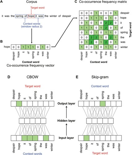
For the present research, given a large corpus of text, the context of a particular target word t is the collection of words within some fixed distance r of t. The co-occurrence frequency vector for t is a list, for each word c in the corpus vocabulary, of the number of times c is found in the context of t. Thus, for a context window of radius r, the co-occurrence frequency vector for t has entries $n_r(c,t)$ indexed by the unique words in the corpus. Note that in this definition, the words order in the context does not affect the resultant values. Vectors are compiled over target words into a co-occurrence frequency matrix whose rows are indexed by the unique words in the corpus as targets and whose columns are indexed by unique words as context. For context windows which are symmetric around the target word, this matrix is symmetric when target and context words are arranged in the same order. See Figure 1 for an illustrative example of how a co-occurrence frequency matrix is computed.

Figure 1. Schematic architectures of vector-based count and predict model families, trained on a small corpus with a context window of radius 2. In count vector models A–C, each word in the corpus is selected in turn as a target and words falling within a fixed radius of the target are selected as context words (A). The frequency of co-occurrences within the corpus of the target word and each context words are recorded in a vector (B), and vectors for each target word are compiled into a co-occurrence frequency matrix (C). In predict models D–E, either an aggregate of all context words is used to predict the target word (D: CBOW), or the target word is used to predict each context word (E: Skip-gram). Networks are feed-forward and fully connected; these schematic representations are a simplification of the implementation details of CBOW and skip-gram in Word2vec (see Mikolov, Chen, et al., 2013).

We considered four count vector models that differ in their transformation of the co-occurrence frequency matrix. For each of these models, we let r take values 1, 3, 5 and 10. This choice spans the range of popular and high-performing window sizes (J. Levy et al., 1999; O. Levy et al., 2015; Mandera et al., 2017).

• Log co-occurrence frequency: Log frequency is often used in place of raw co-occurrence-counts as a better-performing alternative that compensates for the skewed distribution of word frequencies in language (e.g. Louwerse & Connell, 2011). The log co-occurrence frequency model has word vectors defined as the log-transformed frequency count of finding a context word c and target word t together within a context window of radius r:

  $l_r(c,t)={\log }_{10}(n_r(c,t)+1)$

  The $+1$ is a smoothing term which lets the model be defined even where $n_r(c,t)=0$ (i.e. where the co-occurrence frequency is zero).

• Conditional probability: The vector components of the conditional probability model are the probability of finding a particular context word c, given the target word t, within a context window of radius r:

  $p_r(c|t)={\displaystyle \frac{p_r(c,t)}{p_r(t)}}$

  Here, $p_r(c,t)=n_r(c,t)/kr$ is the probability of finding a particular context–target pair, where k is the size of the corpus, and $p_r(t)={\sum }_c{n}_r(c,t)/kr$ is the probability of finding a given target word.

• Probability ratio: The ratio of probabilities model compares the probability of finding a context c and target t together to the probabilities of finding c and t separately (Bullinaria & Levy, 2007):

  $\mathrm{rati}{\mathrm{o}}_{\mathrm{r}}(c,t)={\displaystyle \frac{p_r(c,t)}{p_r(c)p_r(t)}}$

  Here, the probability of the context $p_r(c)$ is defined in the same way as the target word probability: $p_r(c)={\sum }_t{n}_r(c,t)/kr$.

• Positive pointwise mutual information (PPMI): Pointwise mutual information (PMI; Church & Hanks, 1990) is an information-theoretic measure defined as the log ratio of probabilities:

  $\mathrm{PM}{\mathrm{I}}_{\mathrm{r}}(c,t)={\log }_2\mathrm{rati}{\mathrm{o}}_{\mathrm{r}}(c,t)$

  PMI is sometimes used directly (e.g. Recchia & Jones, 2009). However, many sources (e.g. Baroni et al., 2014; Bullinaria & Levy, 2007, 2012; Mandera et al., 2017) have found that superior results can be achieved by restricting PMI to positive values (positive PMI; PPMI), thereby only considering word co-occurrences which are more frequent than expected:

  $\mathrm{PPM}{\mathrm{I}}_{\mathrm{r}}(c,t)=max(0,\mathrm{PM}{\mathrm{I}}_{\mathrm{r}}(c,t))$

  PPMI is often selected as the de facto best count model for general tasks in distributional semantics research (e.g. Baroni et al., 2014; Bullinaria & Levy, 2012; Kiela & Clark, 2014; Mandera et al., 2017).

N-gram models

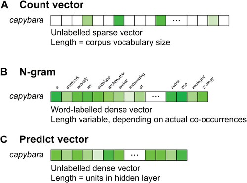
N-gram models have long been employed in corpus analysis, computational linguistics, and cognitive psychology, with Google's Web 1T 5-gram corpus (Brants & Franz, 2006) being a popular recent example.⁵ N-gram models are conceptually simpler versions of count vector models in that they are based on the same underlying method of counting word-to-word co-occurrences. However, there are critical differences in word representation and comparison. Whereas a count vector model represents each word in the corpus as a fixed-length vector of ordered, unlabelled co-occurrences (one dimension for each unique word token in the corpus), an n-gram model represents a word as a labelled list of frequencies for each other word with which it co-occurs in the corpus (see Figure 2 for an illustration). It is important to note, therefore, that two words can only be meaningfully compared using an n-gram model if they have actually occurred at least once within the same context window; otherwise, the co-occurrence frequency is automatically zero (i.e. target word and context word never co-occurred).

Figure 2. Word representation in each model family. A: In a count vector model, a word's representation is an unlabelled, sparse vector of length equal to the number of unique words in the corpus. B: In an n-gram model, a word's representation is a labelled, dense list of nonzero co-occurrences whose length varies with the diversity of co-occurring words. C: In a predict vector model, a word's representation is an unlabelled, dense vector of length equal to the size of the neural network's hidden layer (i.e. its embedding size).

We consider three n-gram models that differ in their transformation of co-occurrence frequencies. In general, n-gram models use the same method for constructing the co-occurrence frequency matrix as count vector models; as with the count vector models, we let window radius r take values 1, 3, 5 and 10. Since the n in n-gram comprises a sequence of the target word plus its surrounding context words, these window radii correspond to 2-, 4-, 6-, and 11-grams.

• Log n-gram frequency: Based on the same calculations as the log co-occurrence frequency count vector model, this model defines the relationship between two words t and c as their log-transformed co-occurrence frequency within a context window of radius r.

• Probability ratio n-gram: Based on the same calculations as the probability ratio count vector model, this model defines the relationship between two words t and c as the probability of finding them together within a context window of radius r compared to the probabilities of finding them separately within the corpus.

• PPMI n-gram: Based on the same calculations as the PPMI count vector model, this model defines the relationship between two words t and c as their log-transformed probability ratio, with negative values treated as zero.

Predict models

Many modern predict models are based on artificial neural network architectures, including those implemented in the popular software tool Word2vec (Mikolov, Chen, et al., 2013). These models are realised as neural networks that map between context and target words with a single hidden layer, illustrated schematically in Figure 1, where words are represented in input and output layers by Huffman codes. Predict models are also vector models, where the vector representation of a target word comprises the row of weights between the input layer and the hidden layer.

We consider two predict models that differ in their direction of prediction.⁶ As with the count vector models, we let r take values 1, 3, 5 and 10 during training; though as is usual for implementations of such models, the actual width of the window before and after the target word at each training step is randomly selected from $\{1,\dots ,r\}$.

• Continuous bag of words (CBOW): This model is trained to predict the target word from the unordered collection of the context words. The mean of the context words’ codes is used as input (Mikolov, Chen, et al., 2013).

• Skip-gram: This model is trained to predict each of the context words separately from the target word, and effectively reverses the learning direction of CBOW.

There are a great many potential parameters available for predict models. The most obvious is the specific architecture of the neural network, namely the number of units in its hidden layer. This is the embedding size, denoted e. Unlike count vector models, neural network-based predict models must implicitly perform dimensionality reduction whenever the hidden layer is smaller than the input layer, which will always be the case for the models we employ in this paper. For each of the models below, we trained with $e=50,100,200,300,500$, matching values used by Mandera et al. (2017). The Word2vec implementations of CBOW and skip-gram models have further optimisation and regularisation steps which have been found to improve performance (Mikolov, Sutskever, et al., 2013). Negative sampling involves updating only a randomly selected subset of network weights at each training step in the negative cases (i.e. words not found in the window), and sub-sampling involves randomly ignoring high-frequency words with a fixed probability. Following the advice of Baroni et al. (2014) and Mandera et al. (2017), we used a fixed value of 10 for negative sampling, and sub-sampled with probability of ${10}^{-5}$. We constructed and trained our predict models in Python 3.7 using version 2.2 of the Gensim package (Řehůřek and Sojka, 2010), which implements CBOW and skip-gram in a manner compatible with the original Word2vec.

Distributional measures between words

Whereas n-gram models represent words as variable-length, labelled “look-up tables”, count and predict vector models both represent words as unlabelled⁷, fixed-dimensionality vectors (see Figure 2). As such, calculating a distributional score or distance between two words requires a different process for vector and n-gram LDMs.

In an n-gram LDM, two words are compared simply by looking up one word's distributional score in the context of the other. For instance, the PPMI n-gram model represents a word such as cat by the collection of words that co-occur with cat within radius $r$, alongside their respective PPMI scores. The words cat and claws can then be compared directly using the value $\mathrm{PPM}{\mathrm{I}}_r(cat,claws)$.

By contrast, in a vector LDM, two words are compared by selecting their respective fixed-dimensionality vector representations in the model and calculating the distance between them using vector geometry. For example, the PPMI count vector model represents a word such as cat by the vector of PPMI values between cat and every other word in the corpus; and the word claws is similarly represented by the vector of all PPMI values between claws and every other word in the corpus. Comparing the words cat and claws involves comparing their respective vectors using some measure of distance in high-dimensional vector space. For count and predict vector models, we therefore use three popular distance measures to compare words’ vector representations⁸:

• Euclidean distance can be regarded as the “natural” straight-line distance measure in a vector space. It is defined as:

  $d_{\mathrm{Euclidean}}(u,v)=\sqrt{{\sum }_i{(u_i-v_i)}^2}=|u-v|$

  While Euclidean distance is widely used (e.g. Lund & Burgess, 1996; Patel et al., 1998), it is affected by the overall magnitude of each word vector and is typically inferior to alternatives which are not affected by vector magnitude (Bullinaria & Levy, 2007, 2012).

• Cosine distance is a widely used distance metric (e.g. Landauer & Dumais, 1997; Mandera et al., 2017; Recchia & Louwerse, 2014) that is normalised by overall vector magnitude (and thus not affected by it). It is defined as:

  $d_{\cos }(u,v)=1-\cos {\theta }_{u,v}=1-{\displaystyle \frac{u\cdot v}{|u||v|}}$

  where ${\theta }_{u,v}$ is the angle between the vectors u and v. For count vector models, cosine distance has often been found to be the best-performing distance metric across a range of tasks (e.g. Baroni et al., 2014; Bullinaria & Levy, 2007, 2012; Lapesa & Evert, 2014). It should be noted that cosine distance, thus defined, is not a true distance metric in the mathematical sense, since it violates the identity-of-indiscernibles and triangle-inequality axioms (see Griffiths et al., 2007; Nematzadeh et al., 2017, for discussion), and is perhaps better thought of as a measure of vector dissimilarity. Despite the technical inaccuracy, $d_{\cos }(u,v)$ is conventionally referred to as a distance, and we follow that convention in the present paper. We note, in addition, that human similarity judgements also may not conform to the axioms for a distance metric (Tversky, 1977; Yearsley et al., 2017).

• Correlation distance is a version of cosine distance with mean centering:

  $\begin{array}{rl}{d}_{\mathrm{corr}}(u,v)& =d_{\cos }(u-{\mu }_u,v-{\mu }_v)\\ & =1-{\displaystyle \frac{(u-{\mu }_u)\cdot (v-{\mu }_v)}{|u||v|}}\end{array}$

  where ${\mu }_u$ and ${\mu }_u$ are the means of u and v respectively. In practice, we found that correlation distance gives almost identical results to the more widely used cosine distance in many scenarios. However, some authors including Kiela and Clark (2014) recommend correlation over cosine as a distance measure for LDMs. Like cosine distance, correlation distance is not a distance metric in the mathematical sense, but nonetheless is commonly used and provides a convenient way to express the dissimilarity of vectors.

Corpora

The distributional properties of words and their contexts are estimated from large corpora of text which are representative of the language to varying extents. The size, quality and source (i.e. spoken or written language) of training corpora have been found to affect the performance of LDMs on various tasks (Bullinaria & Levy, 2012; De Deyne et al., 2015; Mandera et al., 2017; Recchia & Jones, 2009).

We trained LDMs on three corpora that varied in size, quality, and source.⁹ Coming from different sources, each corpus required both individual and shared cleaning and pre-processing steps (detailed below). All corpus processing was done using Python 3.7 and version 3.2 of the Natural Language Toolkit software library (NLTK; Bird et al., 2009).

• BNC: The British National Corpus (BNC; BNC Consortium, 2007) is a very high-quality corpus of 100 million words of spoken and written language. It represents a collection of 4,049 documents of British English language from the early 1990s, collected from a variety of sources, and includes approximately 90 million words of written language and 10 million words of spoken language (both prepared and spontaneous speech). It is a professional corpus of a high quality that was designed to be representative of modern British English. It has been widely used to train LDMs (e.g. Landauer & Dumais, 1997; Bullinaria & Levy, 2007; Levy & Bullinaria, 2001; McDonald, 2000; Patel et al., 1998). The BNC is provided as a collection of XML files, including document metadata and part-of-speech tagging. A schema for automatic removal of all non-textual tagging is also available from the Oxford Text Archive (2009), yielding a corpus of plain-text documents.

• Subtitles: The Subtitles corpus is a reasonably high-quality corpus of 200 million words of spoken language, representing a collection of subtitles from 45,099 television programmes and films broadcast by the British Broadcasting Corporation (BBC) channels in the period 2010–2012. A corpus of BBC subtitles was first used to compile the SUBTLEX-UK database of word frequencies, which outperformed BNC word frequencies in predicting word recognition performance (van Heuven et al., 2014). The programmes contain a mixture of scripted and unscripted (i.e. spontaneous) speech for audiences ranging from newborn to adult, across a wide range of topics and genres. It is a high-quality corpus, having been professionally transcribed, although it was not explicitly designed to be representative of British English. Raw subtitle files contain many elements apart from the words spoken during the broadcast, such as non-linguistic descriptions of events and sounds taking place, and numeric mark-up describing the order and timing of utterances. As well as removing all timestamps and associated formatting elements, we removed segments which were likely descriptions of sounds, events or metadata (e.g. LAUGHTER AND APPLAUSE or Subtitles by Red Bee Media Ltd). Two documents were excluded for containing invalid formatting.

• UKWAC: The United Kingdom Web as Corpus (UKWAC; Baroni et al., 2009) is low-quality corpus of approximately 2 billion words of written language. It comprises text scraped from webpages with .uk domains between 2005 and 2007, where medium-frequency words from the BNC were used as seed words to select pages. It is provided as a collection of plain text files (without HTML markup) and associated source metadata. UKWAC is much larger than the other two corpora, but has been subjected to minimal quality control and therefore contains a much higher level of noise, including typos (e.g. htink instead of think), misspellings (e.g. dissapear instead of disappear), and run-together words (e.g. wantto instead of want to). It has previously been used to train LDMs, particularly predict models (e.g. Baroni et al., 2009; Bullinaria & Levy, 2012; Mandera et al., 2017; J.P. Levy et al., 2017; O. Levy et al., 2015; Pereira et al., 2016). We removed all source metadata prior to further processing.

We processed all three corpora as consistently as possible. After the individual pre-processing steps described above, all corpora were tokenised using the Penn Treebank word tokenizer in NLTK, modified to account for additional non-alphanumeric symbols found with high frequency in the corpora (e.g. £). Resulting tokens were converted to lower case, and most grammatical punctuation was removed. Further details of the tokenization procedure are available in supplementary materials.

Other commonly used corpus pre-processing steps include the removal of low-frequency tokens (Bullinaria & Levy, 2007; Levy & Bullinaria, 2001; Lund & Burgess, 1996; Mikolov, Chen, et al., 2013; O. Levy et al., 2015), and the removal of high-frequency tokens or those appearing in a “stop list” (Bullinaria & Levy, 2012; Lowe & McDonald, 2000; Rapp, 2003; Riordan & Jones, 2011). This is often done to reduce computational cost, but after a thorough investigation, Bullinaria and Levy (2012) found that doing so led to little performance gain over several evaluation criteria. Since we were able to complete all computations without pruning linguistic tokens from the corpus, we did not use such approaches in order to retain maximum vocabulary coverage for the evaluation procedures, and to avoid making psychologically unmotivated alterations to the LDM algorithms.

Evaluation tasks

Since our goal was to examine the efficacy of LDMs in fitting human data across a range of cognitive tasks, we required a suite of tasks which (a) used words as stimuli, (b) involved access to semantics (i.e. conceptual processing), and (c) varied in the complexity of their conceptual processing and use of implicit vs. explicit dependent measures. In order of increasing conceptual complexity (i.e. operationalised as greater diversity of semantic relations in the stimulus set, greater reliance on syntagmatic over paradigmatic relations, and greater reliance on bag-of-words relations over syntagmatic and paradigmatic), we selected the following five tasks: synonym selection (Study 1), similarity and relatedness judgement (Study 2), thematic relatedness production (Study 3), semantic priming (Study 4), and semantic decision (Study 5). Studies 1–3 involve explicit task responses as dependent measures (e.g. ratings, word choice), Study 4 involves an implicit measure of processing effort (i.e. response times), and Study 5 involves both. Table 2 summarises the task characteristics, and each one is described in more detail in its relevant study below.

Table 2. Overview of evaluation tasks.

Task	Conceptual complexity	Processing measure
Study 1: Synonym choice	Very low	Explicit
Study 2: Similarity rating	Low	Explicit
Study 2: Relatedness rating	Medium	Explicit
Study 3: Thematic relatedness production	Medium–high	Explicit
Study 4: Semantic priming	High (but variable)	Implicit
Study 5: Semantic decision	Very high	Explicit and implicit

Study 1: Synonym selection

Synonym-finding tests consist of multiple-choice questions where a seed word is presented (e.g. rusty), and the test-taker must select from a list of candidate synonyms the option which is closest in meaning to the seed (e.g. corroded, black, dirty, painted; in this case, corroded is the correct choice). LDM performance in these tasks is based on comparing the seed word to each candidate synonym, where the candidate with the best score is selected and evaluated according to its fit to objective accuracy (i.e. the correct synonym choice per seed: an explicit measure of semantic/conceptual processing) rather than to human data per se. As a task, synonym selection relies strongly on a single semantic relation (i.e. synonyms) that can be learned paradigmatically (e.g. the structures rusty metal and corroded metal allows the rusty–corroded synonymic relation to form), which makes it a conceptually simple task.

In this and the following studies, since each of our 540 candidate LDMs is tested on multiple datasets, there is a very large volume of results. As such, we concentrate in the results section on describing the best-performing models and summaries of overall trends. Full results are available in the online materials.

Method

Materials and datasets

We modelled three separate synonym selection tests that differ in their construction and difficulty.

TOEFL

The Test of English as a Foreign Language (TOEFL; Institute of Cognitive Sciences, University of Colorado Boulder, Boulder CO, 1989) is a test undertaken by American college entrants to evaluate their English vocabulary. It includes 80 four-way multiple-choice questions comprising a mixture of low- and high-frequency words. It is widely used as a benchmark for LDMs (Baroni et al., 2014; Bullinaria & Levy, 2007, 2012; Kiela & Clark, 2014; Landauer & Dumais, 1997; Mandera et al., 2017; Rapp, 2003; Recchia & Jones, 2009). For instance, when used by Landauer and Dumais (1997), LSA achieved a score of 64%, which was approximately the average score of non-native English-speaking university applicants taking the test. With a careful choice of parameters, Bullinaria and Levy (2012) later managed to achieve a perfect score.

We used TOEFL as it was used by Landauer and Dumais (1997) and Bullinaria and Levy (2007, 2012), with a few American-English spellings replaced by their British-English counterparts (e.g. recognized replaced with recognised), since all three of our corpora are from predominantly British sources.

ESL

The English as a Second Language test (ESL; Tatsuki, 1998) is a multiple-choice test for non-native speakers of English. It consists of 50 four-way multiple-choice questions comprising mainly higher-frequency and some lower-frequency words. It is used as an LDM benchmark (e.g. Jarmasz & Szpakowicz, 2004; Recchia & Jones, 2009; Terra & Clarke, 2003; Turney, 2001), though less widely than TOEFL.

We altered one term of the ESL test to remove a function word (a hurry was replaced by hurry). We also omitted one question as containing a two-word term (unwanted plant as a synonym for weed).

LBM: Levy et al.’s (2017) test

J. Levy et al. (2017) have proposed a new multiple-choice synonym test for the evaluation of LDMs and other linguistic models, which improves on replication difficulties found with other synonym tests, and over-reliance on a small collection of evaluation datasets in the literature. It consists of 200 four-way multiple-choice questions with a mixture of high- and low-frequency words (Bullinaria, n.d.).

Evaluation procedure

For both count vector and predict models, we computed the distance between the vector representations of the seed word and each of the choice words, and selected the choice with the smallest distance. In any cases where a seed word was not found in the corpus, the question was marked as incorrect, and in any cases where a choice word was not found, it was assigned an infinite distance that guaranteed it would not be selected. Where there were ties between choice words for smallest distributional distance, we selected the last-found item as the model answer.

For n-gram models, the choice word with the largest distributional score relative to the seed word was selected. In any cases where a seed word was not found in the corpus, the question was marked as incorrect. In any cases where a choice word was not found within the seed word’s collection of co-occurring words (i.e. either because it never co-occurred with the seed or because it was not in the corpus), it was assigned the minimum distributional score of zero for the model. Ties between choice words for largest distributional score were resolved as above.

Performance for each LDM was calculated as the percentage score of correctly identified synonyms per dataset. For the score achieved by each LDM, we computed a Bayes factor BF₁₀ for the alternative hypothesis that the model was performing above chance against the null hypothesis that it was performing at chance level, by modelling the score as binomially distributed $\mathrm{Binom}(n,p).$As each test set consisted of four-way multiple-choice questions, the null hypothesis H₀ was that $p=1/4$in each case, with the alternative hypothesis H₁ being $p>1/4$, with an uninformative one-tailed beta distribution prior on p (Wagenmakers, 2007). In this and future studies, when determining optimal models, corpora, and parameters, we considered one LDM₁ superior to another LDM₂ if the data were at least 10 times more likely to occur under LDM₁ (i.e. model comparison BF₁₂ ≥ 10; see Jeffreys, 1998). Our key optimality criterion was robustness of performance: for example, a particular window radius r would only be considered optimal if it produced superior performance for a range of LDMs and corpora, and thus could reasonably be expected to generalise well.

Results and discussion

LDM performance for synonym selection was overall at its best for a context window size of 1 (although of r = 3 was comparable or better for some of the best-performing LDMs). Cosine and correlation distance produced almost identical results in most instances, greatly out-performing Euclidean distance, but cosine distance had the edge amongst the best-performing LDMs. Results for all models can be found in the online materials and are summarised in Figure 3; performance for each model using the optimal parameters (context window size 1, cosine distance) is shown in Figure 4 and forms the basis for the wider trends and recommendations reported below.

Figure 3. Violin plots showing the performance of each LDM at modelling each dataset in Studies 1–5. One distribution is shown for each model type, summarising results of all corpora, window radii, and where relevant embedding sizes and distance types. Circular dots show LDMs whose performance was substantially preferred to the null model (BF₁₀ ≥ 10: Jeffreys, 1998), and × marks show LDMs whose performance was equal to or worse than the null (BF₁₀ < 10). Dots are filled black where the LDM had optimal parameter values (see Table 3), grey where one parameter has a non-optimal value, and unfilled where the LDM has 2 or more non-optimal parameter values. Note that optimal LDMs are chosen for robustness across parameters so top-performing outliers may not represent the optimal choice for a given task. Horizontal red lines (where visible) show performance at the level of chance.

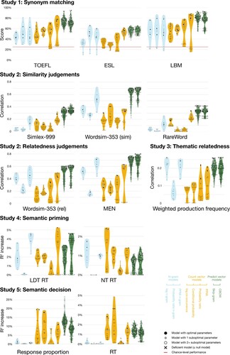
Figure 4. LDM performance per corpus and dataset in Study 1’s synonym selection task, for optimal parameters of window radius $r=1$ and cosine distance between vectors. Panel A shows scores as percentage accuracy, where horizontal red lines indicate chance performance. Panel B shows log Bayes factors (Log₁₀ BF₁₀) for LDM performance; positive values indicate evidence favours the LDM over the null model, negative indicate evidence favours the null model over the LDM, and the dotted horizontal lines indicate the Log₁₀ BF₁₀= 1 (i.e. BF₁₀ = 10) threshold for strong evidence (Jeffreys, 1998).

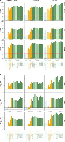
LDM behaviour was relatively consistent across synonym datasets. At optimal parameter settings, scores were very high on TOEFL and LBM, while scores for ESL were generally much lower. Across all datasets, there was extremely strong evidence in favour of using the best LDMs to select synonyms (all BF₁₀ > 1.0×10⁹⁰). Not every parameter setting performed equally well, with some (e.g. log n-gram model trained on the BNC with radius 1 using cosine distance) performing no better than chance on all datasets.

In terms of model family, predict models generally outperformed count and n-gram models, with the best predict models at optimal parameters achieving up to 95% scores on TOEFL, 93% on LBM, and 60% on ESL. Of the predict models, both skip-gram (at r = 1) and CBOW (at r = 1 or 3) performed equally well overall, and while larger embedding sizes tended to achieve better results, in both cases the best performance was found at e = 300. Of the count models, PPMI generally performed the best, corroborating the findings of Bullinaria and Levy (2007, 2012). Notably, with optimal parameters, the PPMI count vector model was close to competitive with the best predict models for two datasets (achieving 85% on TOEFL, 89% on LBM) and competitive on one (achieving 60% on ESL). N-gram models were highly sensitive to parameters but overall tended to perform worst at synonym selection. However, n-gram models performed well when trained on UKWAC and at certain parameters occasionally beat the optimal predict model (e.g. probability ratio n-gram model using UKWAC at r = 3 achieved the top score of 68% on ESL). Nonetheless, this n-gram success was not representative of overall trends in synonym selection performance and it is therefore unlikely to generalise well.

The UKWAC corpus overall produced the best performance for synonym selection. Although models trained on the different corpora yielded broadly similar patterns of results, UKWAC tended to do substantially better than BNC, a trend also observed by Bullinaria and Levy (2012). The Subtitles corpus performed a little better than the BNC, but still substantially worse than UKWAC. The advantage of UKWAC was particularly evident for the optimal family of predict models and for n-gram models.

In summary, the optimal LDM for the relatively simple, explicit task of synonym selection appears to be either skip-gram or CBOW predict model at a large embedding size of 300, trained on a very large but noisy UKWAC corpus of written language, with a small window radius (either skip-gram at r = 1 or CBOW at r = 1 or 3), and using cosine distance between vectors. The next-best choice is the PPMI count vector model at the same parameters. In Bayesian terms, the optimal predict models were between BF = 1.00 and 1.48×10¹³ times better (depending on dataset) than this next-best choice.¹⁰ In many ways, these findings are unsurprising: LDMs that are optimised to capture paradigmatic relations (i.e. predict models) excel at predicting data in a task that relies on paradigmatic relations (i.e. synonym selection). For the conceptually simple task of synonym selection, our findings support the most common recommendation in distributional semantic research: using predict models trained on a very large corpus of noisy written text.

These recommendations are consistent with previous findings for synonym selection (e.g. Bullinaria & Levy, 2007, 2012; Mandera et al., 2017). Nonetheless, there are some instances where our findings differ from previous research for apparently the same LDM, parameter settings, and dataset. For instance, Bullinaria and Levy (2007) achieved accuracy of 83% on the TOEFL dataset using a radius-1 symmetric-window PPMI model trained on the BNC, for which we achieved 79% using the same parameters. The reason for this discrepancy in performance is due to differences in corpus pre-processing and tokenization steps: we use single-word tokenization (i.e. bag-of-words approach), whereas they used a more sophisticated tokenization strategy based on BNC part-of-speech tags.¹¹ As we wished to retain a consistent bag-of-words approach in order to examine how LDM appropriateness varied systematically across models, corpora, and tasks, we did not further explore tokenization strategies that could not be applied uniformly across all corpora. However, researchers interested in optimising LDM performance for one particular task may be able to enhance performance by tweaking their corpus pre-processing strategies.

Study 2: Similarity and relatedness judgements

Datasets of direct human similarity judgements are another common way to evaluate LDMs. They typically consist of responses from human participants to the task of rating the similarity or relatedness of pairs of words, and as such represent an explicit measure of semantic or conceptual processing. In the context of such judgements, semantic similarity is a relatively specific measure of the degree to which two words or concepts resemble each other in meaning (e.g. student–pupil, old–new, king–queen), whereas semantic relatedness is a more general construct that reflects the degree to which two words or concepts are connected via a functional, thematic, or other relation (e.g. grapes–wine, river–water, physics–proton). LDM performance in these tasks is based on comparing each word pair (e.g. king–queen) to produce a distributional measure, and then evaluated by correlating these LDM measures with the corresponding human similarity or relatedness rating (see Wingfield & Connell, 2022, for an overview of alternative theories and measures of semantic similarity).

Both tasks are more conceptually complex than the synonym selection task of Study 1. Although similarity judgements clearly rely on similarity of meaning, which is paradigmatically learned (e.g. the structures hard exam and difficult exam allow the hard–difficult synonymic relation to form), words are often rated as highly similar despite having distinctly different referents (e.g. king and queen; old and new). For example, the structures king’s palace and queen’s palace allow the king–queen categorical relation to form, or old hat and new hat allow the old–new antonym relation to form. Similarity judgement tasks are therefore a little more conceptually complex than the synonym selection task of Study 1 when they use a more diverse variety of paradigmatic relations. Relatedness judgements are more complex again due to their broader use of a variety of relations that go beyond paradigmatic alone. The stimuli of relatedness judgements sometimes overlap with similarity judgements in their use of paradigmatic relations (e.g. king–queen are categorically related; money–wealth are synonymically related), but they also feature syntagmatic relations (e.g. river–water are compositionally related and comprise a noun-noun phrase), and other bag-of-words relations (e.g. physics–proton are thematically related but do not neatly fit paradigmatic or syntagmatic forms).

Method

Materials and datasets

We modelled four separate similarity and relatedness datasets tests that differ in their instruction to participants.

Simlex-999

The Simlex-999 dataset (Hill, n.d.; Hill et al., 2015) consists of similarity ratings on 999 word pairs. Participants were instructed to rate word pairs on similarity only, and disregard relatedness ($N=50$ per pair). Simlex-999 has previously been used to evaluate LDMs (O. Levy et al., 2015; Mandera et al., 2017; Nematzadeh et al., 2017; Pereira et al., 2016).

WordSim-353

The WordSim-353 dataset (Finkelstein et al., 2002; Gabrilovich, 2002) consists of composite similarity/relatedness ratings from human participants on 353 word pairs ($N=13$ or $N=16$ per pair). This set of word pairs was split post-hoc by Finkelstein et al. into subsets that were linked by either semantic similarity (WordSim-353-similarity: 203 pairs) or relatedness (WordSim-353-relatedness: 252 items; 102 pairs were included in both lists). WordSim-353 has previously been used to evaluate LDMs (Agirre et al., 2009; Baroni et al., 2014; Kiela & Clark, 2014; Mandera et al., 2017; Pereira et al., 2016).

RareWord

The RareWord dataset (Luong, n.d.; Luong et al., 2013) consists of participants’ similarity ratings on a Likert-style scale for 2034 word pairs ($N=10$ per pair). The word pairs in the RareWord dataset were specifically chosen to focus on low-frequency words such as apocalyptical→prophetic, and were constructed based on WordNet synonym sets. It has previously been used to evaluate LDMs (Pennington et al., 2014; O. Levy et al., 2015).

MEN

The MEN dataset (Bruni, 2012; Bruni et al., 2014) consists of human similarity judgements on 3000 word pairs (N per pair not reported). It has been used to evaluate LDMs (Baroni et al., 2014; Kiela & Clark, 2014; Pereira et al., 2016). Unlike Simlex-999, WordSim-353 and RareWord, which use Likert-style rating scales, MEN scores are computed from a forced-choice paradigm where participants picked the most closely related word pair from two possible options (e.g. wheels:car and dog:race). Nevertheless, the MEN dataset can be modelled in the same way as the others.

Evaluation procedure

For both count vector and predict models, we correlated distributional distances between each word pair with mean participant similarity/relatedness ratings. For n-gram models, distributional scores between word pairs were correlated with participant similarity/relatedness ratings. In cases where a test word was not found in the corpus, we treated it as missing data for the purposes of the correlation. Since a better fit results in negative correlation for count vector and predict models (high similarity/relatedness corresponding to low distance) and positive correlation in the case of n-gram models (high similarity/relatedness corresponding to high distributional score), we report absolute Pearson’s correlation values for ease of cross-comparison.

In addition to the correlation values, we computed Bayes information criterion (BIC, also known as the Schwarz criterion: Schwarz, 1978) values for a single-predictor linear regression of human ratings on each LDM predictor (alternative hypothesis) and an intercept-only baseline regression (null hypothesis). From BIC values, we estimated Bayes factors for the inclusion of the LDM predictors (Wagenmakers, 2007, p. 796).

Results and discussion

The optimal parameters for similarity judgements (Simlex-999, WordSim-353-similarity and RareWord) and relatedness judgements (WordSim-353-relatedness and MEN) differed markedly so we report and discuss them separately. For similarity judgement datasets, LDM performance was best for smaller sizes of window radius r and overall optimal at r = 1, using either correlation or cosine distance (both of which greatly outperformed Euclidean distance). For relatedness judgement datasets, the best LDM performance was for larger sizes of window radius r and optimal at r = 10, using either correlation or cosine distance (both of which substantially outperformed Euclidean distance). Performance for each model using these optimal parameters is shown in Figures 5 and 6, and forms the basis for the trends and recommendations reported below; results for all models can be found in the online materials and are summarised in Figure 3.

Figure 5. LDM performance per corpus and dataset in Study 2’s similarity judgement task, for optimal parameters of window radius $\mathrm{r}=1$ and correlation distance between vectors. Panel A shows Pearson's correlation between mean human ratings and LDM score (n-gram) or distance (predict or count vector) per item; absolute values are shown for ease of comparison between model families. Panel B shows log Bayes factors (Log₁₀ BF₁₀) for LDM performance; positive values indicate evidence favours the LDM over the null model, negative indicate evidence favours the null model over the LDM, and the dotted horizontal lines indicate the Log₁₀ BF₁₀= 1 (i.e. BF₁₀ = 10) threshold for strong evidence (Jeffreys, 1998).

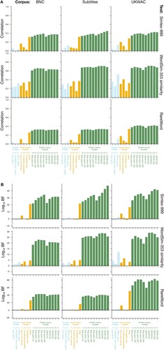
Figure 6. LDM performance per corpus and dataset in Study 2’s relatedness judgement task, for optimal parameters of window radius $r=10$ and correlation distance between vectors. Panel A shows Pearson's correlation between mean human ratings and LDM score (n-gram) or distance (predict or count vector) per item; absolute values are shown for ease of comparison between model families. Panel B shows log Bayes factors (Log₁₀ BF₁₀) for LDM; positive values indicate evidence favours the LDM over the null model, negative indicate evidence favours the null model over the LDM, and the dotted horizontal lines indicate the Log₁₀ BF₁₀= 1 (i.e. BF₁₀ = 10) threshold for strong evidence (Jeffreys, 1998). Note that for the MEN dependent variable (bottom row), the magnitude of the scale means the dotted lines are so close to 0 as to be indistinguishable.

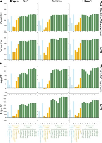
LDM performance varied across datasets. With optimal parameter settings, all model families were able to predict human similarity and relatedness judgements with high accuracy, particularly for the WordSim-353-similarity and MEN datasets (largest magnitude Pearson’s $r$ = .72 and .80 respectively), and more moderately for the RareWord dataset (largest $r$ = .42). Across all datasets, there was extremely strong evidence in favour of using the best LDMs to predict human similarity (BF₁₀ > 1.5 × 10⁴⁷) and relatedness judgements (BF₁₀ > 1.0 × 10³⁰³). Not every parameter setting was viable, however, with some (e.g. Conditional probability count vector model, trained on Subtitles corpus with radius 1, using Euclidean distance, on the Simlex-999 dataset) providing strong evidence for the null hypothesis ($\mathrm{B}{\mathrm{F}}_{10}=0.035$).

Predict models produced the best performance for both similarity and relatedness judgements. In particular, CBOW (at embedding size 300 for similarity judgements and 200 for relatedness judgements) consistently did better than other models, with skip-gram a close second. The next-best model family was n-gram models, where PPMI n-gram was often competitive with skip-gram (particularly for relatedness judgements, and particularly when trained on UKWAC corpus). Log n-gram models also did well for relatedness judgements, if not as well as PPMI n-gram. However, n-gram models did not perform consistently across datasets, with notably poor performance on Simlex-999 and RareWord at optimal parameters. For these datasets, the strongest count vector model (PPMI) greatly outperformed n-gram models, although that pattern did not occur in other datasets.

In terms of corpus choice, similarity judgements overall favoured UKWAC (although both Subtitles and UKWAC corpora were jointly favoured in all but the RareWord dataset), whereas relatedness judgements favoured the Subtitles corpus (with UKWAC lagging some way behind). LDMs trained on the BNC consistently did worse than those trained on either UKWAC or Subtitles corpora. The pattern of LDM performance was generally consistent across corpora, even where it varied by dataset.

In summary, the optimal LDM for relatively simple, explicit similarity judgements closely resembles that for synonym selection: CBOW predict model, at a large embedding size 300, trained on either a very large but noisy corpus of written language (UKWAC), using a small window radius of 1 and correlation or cosine distance between vectors. Alternatively, where the dataset is not primarily composed of low-frequency words, a smaller higher-quality corpus of spoken language (Subtitles) is equally effective at these parameters. Low-frequency words appear to require a larger corpus to achieve adequate lexical coverage (e.g. UKWAC contained 99.2% of words in the RareWord dataset, whereas the otherwise-effective Subtitles corpus contained only 79.7%) and contextual variety (e.g. the smallest corpus BNC contained 90.1% of RareWord items, but nonetheless produced the worst performance). These recommendations are consistent with previous findings for similarity judgements: for example, Mandera et al. (2017) achieved their best results using small context windows (r = 1 or 2), large corpora and CBOW predict models. The consistency of LDM optimality between synonym selection and similarity judgement is unsurprising given that both tasks require a relatively simple form of conceptual processing (i.e. evaluating similarity of meaning). The optimal LDM for slightly more complex relatedness judgements, on the other hand, appears to be CBOW predict model, at a medium embedding size of 200, trained on a medium-sized high-quality corpus of spoken language (Subtitles), using a large window radius of 10 and either cosine or correlation distance between vectors. Bayesian comparisons at optimal parameters showed that these optimal predict LDMs were at least BF = 1.17×10⁶ and 6.61×10¹¹ times better than the top n-gram model (i.e. the second-best model family) for similarity and relatedness judgements, respectively. While similarity and relatedness judgements share many optimal parameter settings, there are some major differences, most notably the jump from a minimal (r = 1) to a maximal (r = 10) window size, and the move away from the large-but-noisy UKWAC corpus towards the higher-quality but smaller Subtitles corpus. These differences may reflect the slightly more complex nature of relatedness judgements compared to similarity judgements, where the paradigmatic link between two words goes beyond similarity of meaning (e.g. strange–odd) and may instead involve locative (e.g. egg–nest), integrative (family–planning), part–whole (flower–petal), or other relations. Many of the highly rated word pairs in relatedness datasets co-occur frequently in text, which is reflected by the competitive performance of PPMI n-gram models in capturing relatedness ratings. Indeed, the datasets where n-gram models perform worst are Simlex-999, the similarity judgement dataset where care was taken to exclude semantic relatedness, and RareWord, where the vast majority of word pairs (78%) are connected in WordNet via hypernymic or similar-to relations rather than broader semantic relations (Pilehvar et al., 2018).

In short, as found for synonym selection in Study 1, semantic tasks that make extensive use of paradigmatic relations (i.e. similarity and relatedness judgements) are best predicted by LDMs that are optimised to capture paradigmatic relations (i.e. predict models). However, when it comes to corpus choice, the present findings diverge from those of Study 1 and are not fully consistent with the typical distributional semantics recommendation of predict models trained on large corpora. Similarity judgements have low conceptual complexity and both a large-and-noisy written corpus (UKWAC) and a medium-sized high-quality spoken corpus (Subtitles) performed equally well. Relatedness judgements have medium conceptual complexity and best served by a medium-sized high-quality spoken corpus (Subtitles). From Study 1–2, increasing conceptual complexity is accompanied by a diversification in corpus recommendations.

However, it should be noted that the distinction between semantic similarity and relatedness is not as clear-cut as the datasets may suggest. In the case of WordSim-353, while the dataset was separated into similarity and relatedness judgements by Finkelstein et al. (2002), the distinction was post-hoc and was not part of instructions given to participants. Similarly, while MEN is described by Bruni et al. (2014) as a relatedness dataset, many of its top-scoring items are near-synonyms (e.g. cathedral–church, cat–feline), leaving the precise distinction between similarity and relatedness unclear. For these and related reasons, some researchers have been highly critical of using human similarity and relatedness judgement data to evaluate LDMs at all (Batchkarov et al., 2016; Faruqui et al., 2016). Nonetheless, given the different patterns of optimal parameters, we preserve the distinction as part of our broader overview of conceptual tasks in the present study.

Study 3: Thematic relatedness production

Thematic relatedness is a form of conceptual relation that is concerned with the complementary roles performed by concepts in a given situation (Estes et al., 2011; Lin & Murphy, 2001). For instance, a fork and a knife perform complementary roles in the scenario of a meal or place setting; an apple and gravity perform complementary roles in the event of Newton’s discovering the principle of universal gravitation. By focusing on how two concepts occupy distinct but complementary roles in a particular time and place, thematic relations include many common semantic relations (e.g. temporal beach–summer, spatial apple–orchard, functional hammer–nail) but exclude others (e.g. synonyms shoes–sneakers, taxonomic flower–rose, and mere association of concepts that never appear in the same situation). Thematic relations therefore represent a form of conceptual information that is critical to many fundamental cognitive tasks, including language comprehension, inference and analogy making, and memory encoding and retrieval (see Estes et al., 2011, for review).

Such conceptual thematic relations largely reflect syntagmatic relations, and in that sense can often overlap with the grammatical sense of thematic relation (i.e. the roles played by the arguments of a verb). For example, cat–mouse may be thematically and syntagmatically related in agent–patient roles (e.g. the cat chased the mouse), and boat–lake may be likewise related in agent–location roles (e.g. the boat floated on the lake). However, some conceptual thematic relations reflect more high-level, abstracted relations that are different to the grammatical roles outlined above. Both apple–gravity and castle–money, for instance, are thematically related in the conceptual sense and are unlikely to be linked paradigmatically or syntagmatically; instead, they constitute bag-of-words relations.

While not typically used for evaluating LDMs (cf. Asr, Zinkov & McRae, 2018), we chose to examine thematic relatedness production as an example of a task that is more conceptually complex than was used in Studies 1 and 2 (by its reliance on a moderately diverse set of syntagmatic and to some extent bag-of-words relations, rather than paradigmatic relations) but is not quite as complex as some of our later tasks, while still representing an explicit measure of conceptual processing. In this task, participants are given a cue word and freely produce a list of target words that are thematically related, which allows each cue-target pair to be scored by rank or frequency of production. Because two words will tend to co-occur in language if their referent concepts co-occur in the real world (Connell, 2019; Louwerse, 2011), we hoped that LDMs would be capable of detecting the thematic relations underlying the responses. LDM performance can then be evaluated by comparing each cue–target pair (e.g. beach–summer) to produce a distributional measure, and then correlating measures with the corresponding human production frequency.

Method

Materials and datasets

We modelled a single dataset of thematic relatedness production norms by Jouravlev and McRae (2016). This dataset consists of 1174 related concept pairs, generated by asking participants ($N=200$) to list thematically related target concepts for 100 cue object concepts. For instance, participants saw the cue concept cat and were asked to write down at least three names of other thematically related objects (i.e. things that might interact with it or be related to it), while avoiding taxonomic responses (e.g. dog: animal). The dataset contains a list of thematically related concepts for each cue word (e.g. cat: dog, mouse, claws, pet), along with production frequency (i.e. the number of participants who produced each response), the rank order in which the responses were produced (e.g. first, second, or third), and a weighted production frequency that combined the two as an overall measure of strength of thematic relatedness (i.e. concepts produced first were weighted more heavily than those produced second, and so on). We used the weighted production frequency as our dependent variable.

Evaluation procedure

For predict and count vector models, we calculated the distance between the vector representations of the cue concept and each of its thematically related concepts, and correlated these distances with the corresponding weighted production frequencies. For n-gram models, we calculated the distributional score between the cue concept and each of its thematically related concepts, and correlated the scores with the corresponding weighted production frequencies. We used the dataset as published, having substituted words to account for typos, American-English and multi-word terms (e.g. cotton candy was not found in our British-English corpora, and was replaced by candyfloss). In cases where terms were not found in our corpora and appropriate substitutions could not be found, we omitted the data points. Since a better fit results in negative correlation for count vector and predict models (high relatedness corresponding to low distance) and positive correlation in the case of n-gram models (high relatedness corresponding to high distributional score), we report absolute Pearson’s correlation values for ease of cross-comparison.

As with the similarity judgement datasets in Study 2, we estimated Bayes factors from BIC in a single-predictor linear regression.

Results and discussion

Overall, LDMs performed best with larger values of window radius r, where the optimal value varied between r = 5 and r = 10 depending on model choice (see below). Correlation and cosine distance produced very similar results, and again both substantially outperformed Euclidean distance. Performance for each model using these optimal parameters forms the basis for the trends and recommendations reported below; results for all models can be found in the online materials and are summarised in Figure 7. Model performance for $r=5$ using cosine distance is shown in Figure 3. In general, LDMs did well at modelling thematic relatedness, with the best LDM scores correlating with weighted production frequency at approximately Pearson’s r = .26, which constitutes extremely strong evidence in favour of using LDM scores to predict thematic relatedness production (BF₁₀ > 2 × 10¹⁵).

Figure 7. LDM performance per corpus and dataset in Study 3’s thematic relatedness production task, for optimal parameters of window radius $r=5$ and cosine distance between vectors. Panel A shows Pearson's correlation between weighted production frequency and LDM score (n-gram) or distance (predict or count vector) per item; absolute values are shown for ease of comparison between model families. Panel B shows log Bayes factors (Log₁₀ BF₁₀) for LDM performance; positive values indicate evidence favours the LDM over the null model, negative indicate evidence favours the null model over the LDM, and the dotted horizontal lines indicate the Log₁₀ BF₁₀= 1 (i.e. BF₁₀ = 10) threshold for strong evidence (Jeffreys, 1998).

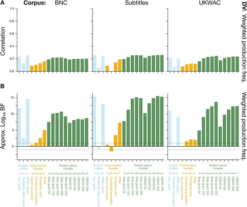
The best model family for thematic relatedness production was tied between predict and n-gram models. With optimal parameters, skip-gram (at embedding size 300 or 500) and CBOW (at e = 500) performed equally well at a window radius of 10, as did log n-gram at r = 5. PPMI n-gram also achieved good results, but was overall not quite competitive with the optimal models. Count vector models (particularly probability ratio and PPMI) performed moderately well in capturing thematic relatedness but nonetheless lagged behind predict and n-gram models.

The Subtitles corpus overall produced the best performance for thematic relatedness across all model families, with UKWAC in clear second place and BNC a distant third. While performance was similar across all corpora at optimal parameters, there were some differential trends in how each model family performed on each corpus. The Subtitles corpus followed general trends with predict models (CBOW and skip-gram) tied with n-gram models (log n-gram) for best performance. When all models were trained on UKWAC, however, predict models did best, and when trained on the BNC, n-gram models did best (though in each case, not as well as when trained on the Subtitle corpus).

In summary, the optimal LDM for a somewhat complex task of thematic relatedness production would appear to be a choice of three: log n-gram trained on a medium-large high-quality corpus of spoken language (Subtitles) with window radius 5, or CBOW or skip-gram at large embedding size 500 (or 300 for skip-gram only), again trained on a medium-large high-quality corpus of spoken language (Subtitles), with window radius 10 and cosine or correlation distance. Performance of these joint-optimal LDMs was indistinguishable in Bayesian terms, where evidence favoured the optimal predict models equally as strongly (BF = 0.44­–1.29) as the optimal n-gram model. In some respects, specifically in the use of predict models trained on the Subtitle corpus with a large window radius, the optimal LDM for thematic relatedness production resembles that of semantic relatedness judgements in Study 2. However, this study is the first indication that something other than predict models emerges as the optimal LDM for a given task: n-grams are also capable of detecting thematic relationships between concepts. Given the much simpler computational load of n-gram models (i.e. count co-occurrence frequencies and transform to distributional score, compare words by looking up score) compared to predict models (i.e. train neural network with supervised learning, compare words by calculating distance between hidden layer vectors), it is remarkable that log n-gram performs as well as CBOW and skip-gram models.

In terms of linguistic distributional knowledge, the present findings show that a semantic task that makes extensive use of syntagmatic relations is best predicted by LDMs that specialise in syntagmatic relations (i.e. n-gram models). However, the task is also equally well predicted by LDMs that are optimised for paradigmatic relations (i.e. predict models). The success of predict models at predicting thematic relatedness, despite their limited capture of syntagmatic relations, has at least two possible explanations. We noted above that thematic relatedness also relies on bag-of-words relations (e.g. computer–internet) in addition to syntagmatic and paradigmatic relations; since both n-gram and predict models can detect these kinds of relations, they may have contributed to their performance in this task. However, count vector models can also detect bag-of-words relations but performed poorly in the task, which suggests that such relations were not a critical component of thematic relatedness production. A more likely alternative is that the success of predict models may be due to the fact that some thematically related words can be connected via similar contexts. For example, knife and fork are thematically related because they often appear together in complementary roles in a dining situation, where such co-occurrence allows n-gram models to score them as highly related, but each word also appears independently in contexts concerning food and dining, where the similarity of these contexts allows predict models to score knife–fork as highly related.

Overall, the findings of this study diverge from the distributional semantics recommendation of predict models trained on large corpora. For the first time, predict models were not the only optimal choice of model family, and – like we found for relatedness ratings in Study 2 – a large but noisy corpus of written text (UKWAC) was not the optimal choice for training LDMs. Thematic relatedness production, as a task of moderate conceptual complexity, is best fit by either n-gram or predict models trained on a medium-sized high-quality spoken corpus (Subtitles). Increasing conceptual complexity appears to be accompanied by some degree of diversification in model family and corpus recommendations.

Finally, it should be noted that this dataset is far less constrained than those of earlier studies. Unlike synonym selection in Study 1 and similarity and relatedness judgements in Study 2, where the word pairs in the datasets were designed by researchers to fulfil certain characteristics, the word pairs in this thematic relatedness task were generated freely by participants. The ability of LDMs to predict such an unconstrained dataset from this moderately complex conceptual task, albeit less accurately than datasets from traditional benchmarking tasks, is testament to the power of linguistic distributional information in predicting a wide range conceptual behaviour.

Study 4: Semantic priming

Semantic priming refers to the phenomenon whereby people are better able to recognise a target word when it is preceded by a word that is related in meaning (see McNamara, 2005; Neely, 1991, for reviews). For instance, people are faster to confirm that tiger is a valid word (lexical decision) or to read tiger aloud (word naming) when it is preceded by related word lion compared to when it is preceded by unrelated word room. In principle, both lexical decision and naming tasks can be performed without any access to semantics (e.g. knowing that “tiger” is a word but “tigen” is not does not necessarily require accessing the meaning of tiger) but in practice the meaning of a word affects how quickly it is processed.

The conceptual complexity of semantic priming depends entirely on the stimulus set used. Synonyms can prime one another (e.g. Perea & Rosa, 2002), such as error→mistake, which indicates that some semantic priming emerges from the same paradigmatic relations that underlie the synonym selection task of Study 1 and the majority of similarity judgements in Study 2. However, semantic priming also includes priming via thematic relations (i.e. prime and target occupy complementary roles in a specific time and place: e.g. L. Jones & Golonka, 2012), such as pillow→blanket, which are syntagmatically or bag-of-words learned, and indicates that it can be as least as conceptually complex as the thematic production task in Study 3. Moreover, semantic priming effects also encompass other complex prime-target relations, including integrative priming (i.e. prime and target can be combined into a coherent whole, such as wool→coat), and taxonomic priming (i.e. prime and target belong to the same taxonomic category, such as lion→tiger), which suggests a level of conceptual complexity beyond that of thematic production. We therefore assume semantic priming in lexical decision and naming tasks has, in principle, a variable level of conceptual complexity that is determined by the stimuli involved. In the present study we chose to use a semantic priming dataset (the Semantic Priming Project: Hutchison et al., 2013) that was quite high in conceptual complexity because its stimulus set featured a diverse set of semantic relations that relied on paradigmatic relations (e.g. synonym error→mistake), syntagmatic relations (e.g. compositional porcelain→doll), as well as more general bag-of-words relations that do not neatly fit either paradigmatic or syntagmatic definitions (e.g. philosophy→thought, ahoy→ship).

Many studies have shown that semantic priming effects can be predicted by the linguistic distributional relationship between prime and target words, both from the perspective of distributional semantics research (M. Jones et al., 2006; Lund et al., 1995; Mandera et al., 2017) and with reference to linguistic–simulation theories of conceptual processing (L. Jones et al., 2017). In the present study, we focus on semantic priming in lexical decision and naming tasks both because of their past history with LDM data and because it offers an opportunity to examine an implicit dependent variable (RT) in a task of reasonable conceptual complexity. Typically, LDM performance is based on comparing each prime→target pair to produce a distributional measure, and then evaluating how well these measures predict human response times to the target word (i.e. whether or not the distributional score can predict the priming effect on the target).

Method

Materials and datasets

We modelled two variables from a single dataset, the semantic priming project (Hutchison et al., 2013), which includes a database of response times to 1611 target words, each preceded by a four different primes, in lexical decision ($N=512$) and word naming ($N=256$) tasks. RT was measured from the onset of the target word to the task-specific response: keypress in lexical decision, or speech onset in word naming. We selected data for 200 ms stimulus onset asynchrony (SOA), the point at which priming effects are elicited automatically, rather than the data for 1200 ms SOA data which incorporates intentional responses strategies (Hutchison et al., 2013). Specifically, we used the mean standardised RT (LDT_200ms_Z and NT_200ms_Z variables from the item-level data files) for each target word following one of four different prime types: first-associate related prime (e.g. lion→tiger) other-associate related prime (e.g. leopard→tiger), first-unrelated prime (e.g. pile→tiger), and other-unrelated prime (plush→tiger).

Evaluation procedure

For predict and count vector models, we calculated the distances from the vector of each prime word to the vector of each target word. For n-gram models, we calculated the distributional score between each prime word and each target word. Each LDM therefore produced a single measure for each prime→target pair, which formed the predictor of interest in linear regression analyses (see below). We made five substitutions to words in the dataset: two from American-English to British-English spelling equivalents (e.g. tumor changed to tumour), two to correct typos (e.g. condfidence changed to confidence), and one to include hyphenation (bookbag changed to book-bag).

To evaluate each LDM, we fit ordinary least-squares linear regressions to each dependent variable (lexical decision RT and naming RT) in two hierarchical steps. Step 1 comprised a set of baseline lexical predictors that affect visual recognition of the target word, extracted from the Elexicon database (Balota et al., 2007): length in letters, number of syllables, log word frequency LgSUBTLWF, orthographic Levenshtein distance OLD20, and phonological Levenshtein distance PLD20.¹² The latter two variables comprise mean Levenshtein distance (Levenshtein, 1966) from the target word to its 20 closest neighbours (Yarkoni et al., 2008).

Any words missing from either our corpora or Elexicon were excluded from the analysis in question (157 items, 2.4% of the total list of prime–target pairs). In addition, we included in Step 1 the orthographic Levenshtein distance (OLD) between prime and target word (e.g. OLD between lion→tiger = 4). Step 2 comprised the critical prime→target predictor for a given LDM (i.e. distributional distance or score from prime word to target word). We then examined the additional variance ($R^2$ change) explained by the LDM predictor in Step 2 compared to Step 1, and estimated Bayes factors for the Step 2 model over Step 1 using BIC, as in previous studies. Zero-order correlations among baseline predictors are available in online materials.

Results and discussion

Overall, LDMs performed best in predicting semantic priming with a medium window of radius 5. In several of the best-performing models, window radius of 3 or 10 did at least as well as radius 5, but it was heavily dependent on corpus choice and task whereas optimal r = 5 performed consistently strongly. Correlation and cosine distance substantially outperformed Euclidean distance, and – although both did equally well in word naming – correlation distance outperformed cosine distance across the best-performing models of lexical decision and was therefore the optimal choice. Performance for each model using these optimal parameters is shown in Figure 8 and forms the basis for the trends and recommendations reported below; results for all models can be found in the online materials and are summarised in Figure 3.

Figure 8. LDM performance per corpus and dataset in Study 4’s semantic priming task, for optimal parameters of window radius $r=5$ and correlation distance between vectors. Panel A shows the increase in $R^2$ achieved by adding a predictor of LDM score (n-gram) or distance (predict or count vector) to a null model containing lexical predictors, in a linear regression of response times per item. Panel B shows log Bayes factors (Log₁₀ BF₁₀) for LDM performance; positive values indicate evidence favours the LDM over the null model, negative indicate evidence favours the null model over the LDM, and the dotted horizontal lines indicate the Log₁₀ BF₁₀= 1 (i.e. BF₁₀ = 10) threshold for strong evidence (Jeffreys, 1998). Note that for the lexical decision RT dependent variable (first row of Panel B), the magnitude of the scale means the dotted lines are so close to 0 as to be indistinguishable.

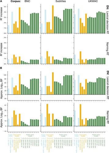
In general, LDMs did very well at modelling semantic priming effects. At optimal parameter settings, the best LDM scores explained up to 5.2% of variance in lexical decision RT (total $R^2$ = .377 including baseline model) and 2.4% of variance in word naming RT (total $R^2$ = .242), which constitutes extremely strong evidence in favour of using LDM scores to predict semantic priming effects (BF₁₀ > 2.11 × 10¹¹² and BF₁₀ > 2.10 × 10⁴², respectively). The finding of larger semantic priming effects for lexical decision compared to naming is consistent with overall patterns in the dataset (Hutchison et al., 2013) and the wider literature (e.g. Balota et al., 2004). By contrast, some parameter settings performed extremely poorly, with their LDMs predicting so little variance (i.e. 0.01% or less) that evidence instead favoured the null model.

The best model family for semantic priming was count vector models, followed by n-gram models, and lastly predict models, though performance varied somewhat by task and corpus. At optimal parameters, semantic priming in lexical decision RT was best modelled by the PPMI count vector model, whereas semantic priming in naming RT was best modelled by log co-occurrence count vector model. While the best LDM for one task still performed reasonably well in the other task – indeed, all count vector models bar probability ratio were good predictors of semantic priming – it was not competitive with the leading LDMs. The second-best LDM for each task tended to be the n-gram equivalent of the best performers (PPMI n-gram for lexical decision; log n-gram for naming), but all n-gram models except for probability ratio n-gram were effective predictors of semantic priming. Predict models (particularly CBOW at embedding sizes from 100 to 500) did well at predicting semantic priming in lexical decision, providing a viable second choice at some parameter settings, but were mediocre at predicting semantic priming in word naming, and hence do not represent a reliable choice.

The Subtitles corpus was the best choice for semantic priming, producing consistently strong performance across LDMs, with UKWAC edging ahead of the BNC for second place according to task and model. While model performance was similar across all corpora at optimal parameters, there were some differential trends in how each model family performed on each corpus. The Subtitles corpus and BNC followed general trends, with count vector models (PPMI for lexical decision, log co-occurrence for word naming) producing best performance. The same pattern appeared for UKWAC in the word naming task. However, when UKWAC was used for the lexical decision task, count vector models did unexpectedly poorly and n-gram models (PPMI n-gram) did best (though overall performance was still not as good as when trained on the Subtitles corpus). Overall, while both the BNC and UKWAC were occasionally competitive with optimal Subtitles corpus for certain LDMs, their performance was too variable to generalise well.

In summary, the optimal LDM for semantic priming seems to be a count vector model trained on a medium-large high-quality corpus of spoken language (Subtitles) with a medium window radius of 5, using correlation distance between vectors. However, the optimal count vector model depends on the exact task used to elicit semantic priming effects. If participants are asked to perform lexical decision, then PPMI is the optimal choice, but if asked to perform word naming, then log co-occurrence is the optimal choice. In Bayesian terms, these optimal count-vector LDMs were clear leaders, performing BF = 2.51 × 10¹⁸ and 1.23 × 10¹⁸ times better than the next-best model family (n-gram models at optimal parameters), for lexical decision and naming times, respectively. These optimal models can explain up to 5.2% of lexical decision time variance and 2.4% of naming time variance, which is comparable to previous investigations of LDMs in semantic priming (e.g. M. Jones et al., 2006; Mandera et al., 2017).¹³ In the event that theoretical or practical reasons required using the same LDM for semantic priming effects in both lexical decision and word naming, then it is possible to use either optimal model but it comes at a cost of performance: the optimal mode for word naming (log co-occurrence) can still explain 2.1% of variance in lexical decision, and the optimal model for lexical decision (PPMI) can still explain 1.4% of variance in naming. Nonetheless, it remains the case that semantic priming, which reflects all three paradigmatic, syntagmatic, and bag-of-words relations, is best predicted by LDMs that capture all three paradigmatic, syntagmatic, and bag-of-words relations (i.e. count vector models).

The optimal LDM for semantic priming is notably different from the relatively simpler tasks that preceded it in Studies 1–3. In particular, the count vector model family was the strongest performer for semantic priming, despite performing poorly for synonym selection, similarity and relatedness judgements, and thematic relatedness judgements. For the first time, predict models were not the optimal or joint-optimal choice, and in fact came last overall. The recommendations of this study therefore represent a significant departure from the distributional semantics recommendation of predict models trained on large corpora. Semantic priming in lexical decision or word naming – both of which involve variable but generally complex conceptual processing – is best served by count vector models trained on a medium-sized high-quality spoken corpus (Subtitles). Based on the trends from Studies 1–4, increasing conceptual complexity is accompanied by a diversification in both model family and corpus recommendations. At this point in our investigation of linguistic distributional knowledge, our findings have cautiously started to support the tenet of flexibility in linguistic–simulation theories rather than the one-size-fits-all approach of distributional semantics. That is, because both the model family and corpus recommendation have moved away from the original recommendations of Study 1 as conceptual complexity has increased, and because even in the present study the optimal count vector model varied by the task used to elicit semantic priming effects, our findings are consistent with the idea that different conceptual tasks use linguistic distributional knowledge differently and therefore require different LDMs.

Nevertheless, since the present study was our first to use an implicit (RT) rather than explicit (ratings, etc.) measure of conceptual processing, it is possible that some of our recommendations rest on that distinction rather than on increasing conceptual complexity. We address this issue in the next study.

Study 5: Abstract–concrete semantic decision

Semantic or categorical decision tasks have long been used across cognitive psychology, psycholinguistics, and neuropsychology in order to examine conceptual representation and processing (McRae et al., 1997; Rosch & Mervis, 1975; Warrington, 1975). For instance, when presented with the word cat, participants might be asked to decide whether it refers to a concrete versus abstract concept, or a living versus non-living thing, and so on. In particular, the abstract-concrete distinction is arguably the most fundamental in the human conceptual system (e.g. Barsalou & Wiemer-Hastings, 2005; Borghi & Binkofski, 2014; Paivio, 1986; Vigliocco et al., 2009), supported by evidence such as double dissociations in neuropsychological impairments (Breedin et al., 1994; Warrington, 1975).

We chose to examine abstract/concrete semantic decisions for two main reasons. Firstly, it allows us to examine both explicit and implicit dependent variables as a function of the same task: the explicit semantic decision for a given word (i.e. abstract or concrete) and the implicit measure of processing effort in arriving at this decision (i.e. RT). Secondly, abstract/concrete semantic decisions represent the type of conceptually complex task that is often the focus of linguistic–simulation research but rarely features in distributional semantics research. One particular theory from linguistic–simulation research, the linguistic shortcut hypothesis, states that if linguistic distributional information can usefully inform a response in a conceptual task before relatively slower sensorimotor simulation can do so, then people will frequently use it as a shortcut in order to avoid potentially more costly cognitive processing (Connell, 2019; Connell & Lynott, 2013). Hence, while participants could perform an abstract/concrete semantic decision via deep consideration of the ontological categories of “concrete things” and “abstract things” (e.g. degree of sensory information in the referent concept: Connell & Lynott, 2012; Vigliocco et al., 2009), the nature of the task means that participants could instead get away with the computationally cheaper heuristic of responding on the basis of the linguistic distributional relationship between the target word and the words used to label the forced-choice alternatives (i.e. “concrete” and “abstract”). That is, people could perform a semantic decision trial by choosing whichever of the category labels had a stronger linguistic distributional relationship with the target word (e.g. for the target word cat, examine the relationships cat–abstract and cat–concrete and select whichever is a closer fit). LDM performance in semantic decision can therefore be modelled by comparing each target word to concrete and abstract (i.e. target–concrete; target­–abstract) to produce two distributional measures per target, and then evaluating how well these measures predict human decisions and response times.

The nature of the linguistic distributional relationship underlying semantic decision depends on the categories specified as choices, but abstract/concrete semantic decision relies on high-level bag-of-words relations and therefore represents a very high level of conceptual complexity beyond that of previous studies. Deciding whether cat is an abstract or concrete concept relies little on paradigmatic or syntagmatic relations. While paradigmatic relations can help to cluster concepts into taxonomic classes (e.g. the structures he fed the cat and he fed the animal will help the cat–animal paradigmatic relation to form), such neat syntactic substitutability is still quite a step from supporting concrete or abstract category membership (i.e. cat and concrete, or cat and abstract, seldom occupy the same syntactic position across similar sentential contexts). Likewise, syntagmatic relations are of limited use unless a category name and target appear together regularly in the same syntactic structure, which is unlikely for cat and concrete (or indeed cat and abstract). Rather, bag-of-words relations in linguistic distributional knowledge (i.e. those that are neither syntagmatic nor paradigmatic and are instead learned regardless of syntax) will be more useful to abstract/concrete semantic decision: the generalised co-occurrence of cat–concrete (and cat–abstract) in the same or similar contexts, regardless of syntactic structure, informs their linguistic distributional relationship.

Method

Materials and datasets

We modelled two variables from a single dataset, the Calgary semantic decision project (Pexman et al., 2017), that comprises reaction times and accuracies for abstract/concrete semantic decision on 10,024 English words ($N=312$). In the study, participants were instructed to decide whether each presented word represented a concrete or abstract concept in a two-alternative forced-choice (2AFC) task.

For each word, Pexman and colleagues included a number of variables. We used the mean standardised RT (zRT_clean_mean variable from the item-level data file) as an implicit measure of conceptual processing. For an explicit measure, Pexman and colleagues had additionally coded each participant decision as correct or incorrect according to how the word was rated in Brysbaert et al.’s (2014) concreteness norms, and reported the mean proportion correct (ACC variable) per word. However, this coding led to the circumstance where some words were coded as ostensibly low accuracy (e.g. phantom accuracy = .129 as an abstract word, meaning 87.1% of Pexman et al.’s participants thought phantom was concrete rather than abstract), which suggested the distinction between correct and incorrect may be somewhat arbitrary in ontological terms. We therefore opted to represent a more neutral explicit measure of response choice that did not reference a predetermined notion of correctness, and recoded the ACC variable to reflect the proportion of participants who decided each word was concrete. For words coded in the semantic decision dataset as concrete (according to Brysbaert et al.’s norms), we used the accuracy figure unaltered because it already reflected the proportion of participants that judged the item as concrete; for words coded as abstract, such as phantom, we used 1–accuracy to ensure it reflected the proportion that judged the word as concrete.

Evaluation procedure

For predict and count vector models, we calculated the distances from the vector of each target word to the vector of each category name “concrete” and “abstract”, and used these two distances as separate predictors in linear regressions (see below). For n-gram models, we calculated the distributional score between each target word and each category name “concrete” and “abstract”, and used these two scores as separate predictors in linear regressions. We used the dataset as published, with 153 words substituted: 118 from American English to British English spellings (e.g. flavor changed to flavour), 31 to include hyphenation (e.g. smalltime changed to small-time), and 3 synonyms for words which were not found in our corpora (barrette to hairclip, flaxseed to linseed, and teakwood to teak).

To evaluate each LDM, we fit ordinary least-squares linear regressions to each dependent variable (RT and “concrete” response proportion) in two hierarchical steps. Step 1 comprised a baseline model of lexical predictors that affect visual recognition of the target word extracted from the Elexicon database (Balota et al., 2007); any words missing from either our corpora or Elexicon were excluded from analyses. Specifically, we entered the following predictors simultaneously: length in letters, number of syllables, log word frequency LgSUBTLWF, orthographic Levenshtein distance OLD20, and phonological Levenshtein distance PLD20. Zero-order correlations amongst baseline predictors are available in online materials: there were no issues of multicollinearity (all VIFs < 7). Step 2 entered simultaneously the two critical predictors for a given LDM (i.e. distributional distance or score from target word to concrete and target word to abstract).¹⁴ We then examined the additional variance explained by the LDM predictors in Step 2 compared to the baseline model of lexical predictors in Step 1 (reported as $R^2$ change). We also estimated Bayes factors for the Step 2 model over Step 1 using BIC, as in previous studies.

Results and discussion

Optimal parameters differed for implicit measures of semantic decision (RT) and explicit measures (proportion of “concrete” responses), and so we report them separately. For implicit semantic decision RT, the picture was quite straightforward: LDM performance was best at medium window radius r = 5 (although r = 3 also did well), and correlation and cosine both equally outperformed Euclidean distance. For explicit proportion of “concrete” responses, LDM performance was highly sensitive to fine tuning of model-corpus-parameter combinations. The absolute best performance came from skip-gram with maximal embedding size e = 500 (though all embedding sizes performed similarly), trained on the UKWAC corpus with a large window radius of r = 10 and using Euclidean distance between vectors, but few of these parameters (particularly the intersection of Euclidean distance and UKWAC) held true as optimal for other LDMs. The vast majority of other LDMs (including the other predict model, CBOW) tended to perform better with a medium window radius of r = 3 or r = 5, and using correlation or cosine distance, regardless of corpus. As such, we concluded the particular parameter settings of the top-scoring model were not representative of overall LDM behaviour and so were unlikely to generalise well. For proportion of “concrete” responses in semantic decisions, the optimal parameters were therefore r = 3 (though r = 5 also did well), and correlation or cosine distance. Performance for each model using these optimal parameters ($r=5$ for RT and $r=3$ for response proportion, correlation or cosine distance) is shown in Figure 9 and forms the basis for the trends and recommendations reported below; results for all models can be found in the online materials and are summarised in Figure 3.

Figure 9. LDM performance per corpus and dataset in Study 5’s abstract/concrete semantic decision task, for optimal parameters of window radius $r=5$ for response times (RT), and radius $r=3$ for response proportion, and correlation distance between vectors. Panel A shows the increase in $R^2$ achieved by adding predictors of LDM scores (n-gram) or distances (predict or count vector) to a null model containing lexical predictors, in a linear regression of RT or response proportion. Panel B shows log Bayes factors (Log₁₀ BF₁₀) for LDM performance; positive values indicate evidence favours the LDM over the null model, negative indicate evidence favours the null model over the LDM, and the dotted horizontal lines indicate the Log₁₀ BF₁₀= 1 (i.e. BF₁₀ = 10) threshold for strong evidence (Jeffreys, 1998). Note that for the Response decision dependent variable (bottom row), the magnitude of the scale means the dotted lines are so close to 0 as to be indistinguishable.

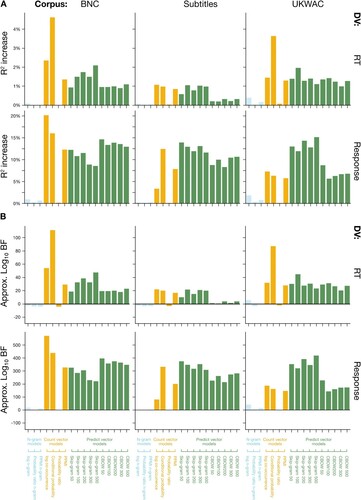
In general, LDMs did well at modelling semantic decision. At optimal parameter settings, the best LDM scores explained up to 4.6% of variance in RTs (total $R^2$ = .198 including baseline model) and 20.1% of variance in the proportion of “concrete” responses (total $R^2$ = .374), which constitutes extremely strong evidence in favour of using LDM scores to predict semantic decision RT (BF₁₀ > 2.15 × 10¹¹¹) and responses (BF₁₀ > 1.11 × 10⁵⁷⁰). Some parameter settings performed extremely poorly, with their LDMs predicting so little variance (i.e. 0.01% or less) that evidence instead favoured the null (baseline) model.

The count vector model family was overall best for semantic decision at optimal parameters, with predict models in second place and n-gram models a distant third. All count vector models bar probability ratio explained meaningful variance in semantic decision, but the optimal model differed by measure. For implicit semantic decision RT, the conditional probability count vector model was best, with the next-best performer (log-co-occurrence count vector model) quite a distance behind. Predict models, particularly skip-gram (optimal embedding size e varied with corpus), performed reasonably well but not competitively, and n-gram models performed poorly. For explicit proportion of “concrete” responses, the log co-occurrence and conditional probability count vector models both performed strongly, with the leader varying by corpus choice (see below). At optimal parameters, however, the top-performing LDM was log co-occurrence. Other strong performers included both skip-gram and CBOW predict models (optimal embedding size varied with corpus), which sometimes beat count vector models depending on corpus, but were overall not competitive with the leading LDMs. As with RT, the n-gram model family tended to perform poorly for response proportion.

In terms of corpus choice for semantic decision, the BNC outperformed other corpora by a clear margin. For both semantic decision RT and responses at optimal parameters, the BNC advantage was consistent across count vector models and across many of the best-performing predict models (note that n-gram models performed too poorly to enable meaningful cross-corpus comparisons). UKWAC was generally in second place and tended to outperform models trained on the Subtitles corpus. However, performance for proportion of “concrete” responses was highly sensitive to model-corpus combinations. For instance, the leading count vector model was log co-occurrence when trained on the BNC or UKWAC, but conditional probability when trained on the Subtitles corpus. In addition, skip-gram predict models tended to perform worst for the BNC, instead favouring the Subtitle corpus at smaller embedding sizes (e = 50–100) and UKWAC at larger embedding sizes (particularly e = 500); however, none were competitive with the best count vector models trained on the BNC.

In summary, the optimal LDM for the conceptually complex task of semantic decision is from the count vector model family, trained on a very high-quality corpus of spoken and written language (BNC) with a small-to-medium window radius, and using cosine or correlation distance between vectors. However, the precise LDM appears to depend on whether the focus of investigation is the explicit task response (i.e. the proportion of participants who selected “concrete” as opposed to “abstract” for a target word) or the implicit measure of processing effort (i.e. the average RT to make the decision). If one wishes to model explicit responses, then the optimal LDM is log co-occurrence count vector model, trained on the BNC with a fairly small window radius of r = 3, and using either cosine or correlation distance. On the other hand, if one wishes to model RT as an implicit measure of processing effort, then the optimal LDM is the conditional probability count vector model, again trained on the BNC, with a medium window radius of r = 5, using either cosine or correlation distance. Other model families do not come close to the performance of these optimal count vector LDMs; at optimal parameters, they are at least BF = 5.50×10⁶³ and 2.82×10¹⁵¹ times better than the most competitive predict models (i.e. the next-best option) for response proportion and RT dependent variables, respectively. In the event that it became important, for reasons of theory or practicality, to use the same LDM for both explicit and implicit measures of semantic decision, then the best compromise would be to use the optimal model for RT (conditional probability); this LDM still did an excellent job predicting response proportions, whereas the reverse was not true to the same extent.

These findings also show that a task that makes extensive use of bag-of-words relations (semantic decision) is best predicted by LDMs that captures bag-of-words relations (count vector models). However, since predict and n-gram models also capture bag-of-words relations, why were they not equally successful at predicting semantic decision? One possible reason may lie in the fact that predict and n-gram models are specialists, with contrasting strengths in capturing paradigmatic and syntagmatic relations, respectively. Count vector models, on the other hand, do not specialise and can capture both paradigmatic and syntagmatic relations (the latter to a slightly lesser extent). We speculate that it may be this compromise of balance in count vector models that allows them to capture bag-of-words relations more effectively than do predict and n-gram models, and hence perform more strongly in predicting conceptual processing that exploits such relations.

Overall, the findings of this study represent a further departure from the distributional semantics recommendation of predict models trained on large corpora. As a task of high conceptual complexity, semantic decision was the first task where the BNC – a relatively small corpus by the standards of distributional semantics but one that is high quality, designed to be representative of language use with low levels of error and noise – was the optimal corpus on which to train LDMs. As in Study 4 on semantic priming, the count vector model family was the strongest performer for semantic decision, despite performing poorly for tasks of lower conceptual complexity. Moreover, these optimal recommendations of count vector model family trained on a small but very high-quality corpus are consistent for both explicit (response decision) and implicit (RT) measures of semantic decision. The trends from Studies 1–5 now show consistently that increasing conceptual complexity is accompanied by a diversification in both model family and corpus recommendations. Rather than a one-size-fits-all approach to modelling linguistic distributional knowledge in cognition, our findings support the idea that different conceptual tasks use linguistic distributional knowledge differently and therefore require different LDMs to capture behaviour.

Finally, we note that the approach taken in this study represents a novel perspective on how linguistic distributional information affects semantic decision tasks. Some previous work had also observed an effect of linguistic distributional information on semantic decision RT, but using a very different method to the one we employed here. Hargreaves and Pexman (2014) used a single variable for each target word that represented the mean distance to all neighbours within a specified distance threshold of the target word (i.e. Shaoul & Westbury’s, 2010, ARC variable), which effectively reflects whether a word appears in a sparse (high score) or dense (low score) area of vector space. They found that semantic decision RT was slightly faster for words in denser vector space compared to sparser vector space. However, this linguistic distributional information pertained to the target word only; they did not examine the relationship between the target word and the words used to label the 2AFC choices (i.e. concrete and abstract) as we did in the present study. The findings we report here – that the distance in vector space between a target word and the words used to label the semantic categories is an excellent predictor of both RT and response decision – suggest that the words used to label category choices in semantic decision tasks (and indeed, any 2AFC tasks with linguistic labels) are at least as important as the target words.

General discussion

Our goal in the present paper was to investigate the role of linguistic distributional knowledge in cognition across a broad set of cognitive tasks, from conceptually simple tasks that rely on similarity of meaning to conceptually complex tasks that require sophisticated processing of diverse and/or abstracted semantic relations. To do so, we conducted the largest to date systematic comparison of linguistic distributional models (LDMs), training corpora, and parameters, and evaluated their ability to predict human data in a range of cognitive tasks that varied in their conceptual complexity. Overall, LDMs were excellent at modelling cognitive behaviour, from highly constrained forced-choice tasks (synonym selection; semantic decision) to highly unconstrained production tasks (thematic relatedness production), in terms of modelling both explicit behaviours such as ratings/decisions (similarity and relatedness ratings; synonym selection; semantic decision) and implicit measures of processing effort such as RT (semantic priming; semantic decision).

However, the optimal LDM differed as conceptual complexity increased; see Table 3 for details of optimal LDM per task, and Figure 10 for a summary of trends. Tasks of low conceptual complexity (Study 1 synonym selection; Study 2 similarity ratings) were best fit by predict models trained on a large but low-quality corpus UKWAC. Tasks of medium conceptual complexity (Study 2 relatedness ratings; Study 3 thematic relatedness production) still found success with predict models but this time trained on a medium-sized, high-quality Subtitles corpus; notably, n-gram models were also competitive here. Tasks of high but variable conceptual complexity (Study 4 semantic priming in lexical decision and naming) were best fit by count vector models rather than predict models, but again with the Subtitles corpus. Finally, a task of very high conceptual complexity (Study 5 abstract/concrete semantic decision) continued the choice of count vector models but this time the small but very high-quality BNC was the optimal training corpus, and these optimal choices held for both explicit (i.e. response proportion) and implicit (i.e. RT) dependent measures of the same task.

Figure 10. Summary of optimal model family and corpus choice for each task in Studies 1–5, according to the conceptual complexity and relevant linguistic distributional relations of each task, and the nature of the dependent measures modelled.

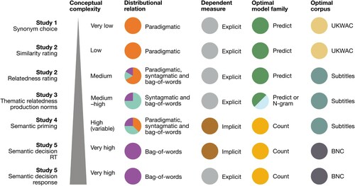
Table 3. Optimal model, corpus and parameters for each task, selected by intersection of parameter settings with best performance quantified by Bayes-factor model comparisons. Where recommendations differ by task or processing measure within a study, we list them separately.

Task	Conceptual complexity	Processing measure	Optimal parameters
			Model family	Model	Corpus	Window radius	Distance
Study 1: Synonym choice	Very low	Explicit	Predict	Skip-gram 300 or CBOW 300	UKWAC	1 or 3	Cosine
Study 2: Similarity rating	Low	Explicit	Predict	CBOW 300	UKWAC	1	Correlation or Cosine
Study 2: Relatedness rating	Medium	Explicit	Predict	CBOW 200	Subtitles	10	Correlation or Cosine
Study 3: Thematic relatedness production	Medium-High	Explicit	N-gram or Predict	Log n-gram or Skip-gram 300–500 or CBOW 500	Subtitles	5 (N-gram) or 10 (predict)	Correlation or Cosine
Study 4: Semantic priming in LDT	High (variable)	Implicit	Count	PPMI	Subtitles	5	Correlation
Study 4: Semantic priming in NT	High (variable)	Implicit	Count	Log co-occurrence	Subtitles	5	Correlation
Study 5: Semantic decision	Very high	Explicit	Count	Log co-occurrence	BNC	3	Correlation or Cosine
		Implicit	Count	Conditional probability	BNC	5	Correlation or Cosine

By contrast, the optimal model family and corpus did not vary systematically according to the implicit versus explicit nature of the dependent measure. Tasks featuring explicit dependent measures that encoded the end result of conceptual processing in the response had no consistent optimal corpus or model family. All three corpora featured as optimal across explicit task measures, from the large but noisy UKWAC (Study 1 synonym selection; Study 2 similarity ratings), to the medium-sized but higher quality Subtitles corpus (Study 2 relatedness ratings; Study 3 thematic relatedness production), to the small but very high quality BNC (Study 5 abstract/concrete semantic decision). All three model families were likewise optimal across explicit tasks: while some were best fit by predict models (Studies 1–2), others were fit equally by both predict and n-gram models (Study 3) or best fit by count vector models (Study 5). Tasks featuring implicit dependent measures of processing effort had no consistent optimal corpus, either continuing the trend started in Study 2 for the Subtitles corpus (Study 4 semantic priming RT) or opting for the BNC (Study 5 semantic decision RT). While implicit task measures shared the same optimal model family, count vector models, they were not alone in that choice. Critically, Study 5 favoured the same optimal model family and corpus (count vector models, BNC) for both its implicit and explicit measures of semantic decision, thus showing that it was a fundamental characteristic of the task (i.e. its conceptual complexity) rather than the explicit vs. implicit dependent measure, that determined optimality.

It is important to note that the selection of optimal model family and corpus were not co-dependent: the optimal model family per task performed robustly across multiple corpora, and the optimal corpus per task performed robustly across multiple model families. Moreover, the changes in optimal choices were not abrupt. For instance, count vector models perform reasonably well throughout Studies 1–3 before dominating in Studies 4–5, and n-gram models perform strongly in Study 2’s relatedness ratings before becoming a joint-optimal choice in Study 3 and then declining to second choice in Study 4. Similarly, the Subtitles corpus first appeared as a joint-optimal choice alongside UKWAC for three out of four similarity datasets in Study 2 before dominating in Studies 3–4, and the BNC appeared as an occasional competitor in Study 4 before dominating in Study 5. Such gradual trends indicate sensitivity to incremental change across Studies 1–5 rather than disjoint model fitting of individual tasks, and suggest that the efficacy of model families and corpora wax and wane systematically according to the conceptual complexity of the task at hand.

Theoretical implications

Our findings suggest that use of linguistic distributional knowledge appears to be ubiquitous in cognition and a vital part of conceptual processing, but it is not an amorphous or rigid resource. Rather, linguistic distributional knowledge is a rich source of information about the world that can be accessed flexibly according to cognitive need. In other words, our findings strongly support a task-dependent flexible approach to the use of linguistic distributional knowledge in cognition rather than a one-size-fits-all approach. Specifically, we found that different conceptual tasks make differential use of linguistic distributional knowledge and therefore require different LDMs to capture behaviour appropriately. No single model family was excellent at all tasks, nor was any single corpus. Rather, tasks of increasing conceptual complexity across Studies 1–5 required increasingly non-specialist models that could capture a wide variety of more abstracted conceptual relations and increasingly high-quality corpora that were representative of human language experience. These patterns are consistent with the tenet of flexibility in linguistic–simulation research, which assumes that linguistic distributional knowledge has a flexible rather than a uniform role in conceptual processing, and that use of such knowledge depends on a number of factors including the nature of the task, surrounding context, and general processing goals (Barsalou et al., 2008; Connell, 2019; Connell & Lynott, 2014; Louwerse, 2011). The present findings contribute to linguistic–simulation theories by showing that the conceptual complexity of a task – that is, whether it relies on a limited range of paradigmatic relations or more diverse and/or abstracted conceptual relations – is a major factor in how linguistic distributional knowledge is used in cognition.

Moreover, our findings shed crucial light on the nature of linguistic distributional knowledge. The large differences in architecture between the model families (i.e. from Hebbian learning to error-driven learning; and from first-order to second-order co-occurrences) translate to large differences in model behaviour: the predictors produced by each LDM per task were poorly correlated between model families.¹⁵ Such differences in distributional estimates indicate that the various model families are not capturing the same latent construct, and that their differences in performance are not simply due to noise. Rather, the relative specialisms of each model family in capturing paradigmatic versus syntagmatic versus bag-of-words relations means that their performance can inform our understanding of how the role of linguistic distributional knowledge varies across cognitive tasks.

Firstly, our findings suggest that syntagmatic, paradigmatic, and bag-of-words relations all underpin the linguistic distributional knowledge that people use in conceptual processing. Many types of conceptual relations can be gleaned from regularities in language experience, including syntagmatic relations (e.g. object properties like blue–eyes; agent actions like customer–pay), paradigmatic relations (e.g. synonyms like error–mistake, shared categories like dog–cat), and bag-of-words relations (e.g. broad thematic relations like philosophy–thought, high-level categories like infinity–abstract). We found that models that specialise in capturing paradigmatic relations (predict models) do best in tasks that rely heavily on paradigmatic relations, such as synonym selection (Study 1) and similarity ratings (Study 2). Conversely, models that specialise at capturing syntagmatic relations (n-gram models) are most useful in tasks that rely heavily on syntagmatic relations, such as thematic relatedness production (Study 3). However, such specialist models are less useful as conceptual complexity increases, and balanced models that capture paradigmatic, syntagmatic, and bag-of-words relations (count vector models) are best for tasks of high conceptual complexity, such as semantic priming (Study 4) and semantic decision (Study 5). In short, conceptual processing makes use of the kind of conceptual relations underpinning linguistic distributional knowledge, but different tasks use each type of relation to different extents. While previous work has argued that people make differential use of linguistic distributional information according to the task at hand (i.e. the tenet of flexibility: see Connell, 2019, for review), such differences are typically presented as quantitative: people make greater or lesser use of linguistic distributional knowledge according to task demands. What we show here is that such differences are also qualitative: as the conceptual complexity of a task increases, the diversity of relevant linguistic distributional knowledge also increases.

Secondly, the present findings suggest that the quality of language experience is highly important to the linguistic distributional knowledge used in conceptual processing, particularly as the diversity of relevant conceptual relations increases. All the corpora we examined were plausible in terms of the quantity of adult language experience (i.e. between 200 million and 2 billion words: see introduction), with the exception of the BNC that was smaller than ideal at 100 million words. Corpus quality, however, varied enormously. We found that large but low-quality corpora like UKWAC, which comprise written text scraped from the web, are most effective when the task to be modelled relies heavily on paradigmatic relations (Study 1 synonym selection, Study 2 similarity ratings). However, UKWAC was less effective than higher-quality corpora when tasks relied on syntagmatic and bag-of-words relations. Instead, the Subtitles corpus, which comprises high-quality transcriptions of scripted and spontaneous spoken language from television and film, was more effective when the tasks to be modelled relied on a mix of paradigmatic, syntagmatic, and bag-of-words relations (Study 3 relatedness ratings, Study 4 thematic relatedness production, Study 5 semantic priming). The BNC, which comprises a very high quality, representative sample of British English across a range of spoken and written sources, was the most effective corpus when the task primarily relied on bag-of-words relations (Study 5 semantic decision), which suggests that the representative nature of the BNC may have compensated for its small size. In other words, it appears that paradigmatic relations can be learned from low-quality language experience that is not representative of the content humans encounter when using language. Syntagmatic relations, however, are better learned from high-quality language experience that is representative to at least some extent of the content humans encounter. And bag-of-words relations, that do not rely on syntactic structures in the same way as syntagmatic or paradigmatic categories but nonetheless reflect broad conceptual themes, seem to have the strongest requirement for high-quality language experience that is most representative of the content humans encounter from a range of language sources. As conceptual complexity increases, the quality of language experience becomes more important than the quantity.

Lastly, our findings suggest that linguistic distributional knowledge is a rich but imperfect source of information about the world (see also Barsalou et al., 2008; Connell & Lynott, 2014; Louwerse, 2011). LDMs were successful at modelling all tasks we examined, but – even allowing for the fact that any LDM is only an approximation of linguistic distributional knowledge – no LDM was without error in modelling a given task. Such model behaviour is entirely consistent with human behaviour: people regularly make mistakes and disagree with one another. For instance, when Battig and Montague (1969) asked people to name as many birds as possible within 30 s in their classic category production norms, they found that people listed concepts such as bat, hate, jail, feathers, pterodactyl, scarecrow, and worm. While such responses may be incorrect – none are birds – they are meaningfully related to birds in a way that tends to be encoded by linguistic distributional knowledge (e.g. jail and bird are syntagmatically related as a compound word; bat and bird are paradigmatically related in terms of flying actions and possessing wings). Any LDM that considers a bat to be a kind of bird would be no more incorrect than some humans.

Even semantic similarity, a mainstay of LDM evaluation, is subject to a high degree of variability in human judgements. For example, Simmons and Estes (2008) found large and robust individual differences in whether people base their similarity judgements on taxonomic or thematic information. When asked to rate the similarity of concept pairs, some participants consistently rated taxonomically related concepts as highly similar (e.g. river and lake) and thematically related concepts as much less similar (e.g. river and boat), whereas other participants consistently showed the reverse pattern, and a third group appeared to vary their preference from one item to the next. The same effects emerged even more strongly when participants were explicitly asked to choose which of two options (e.g. lake or boat) was most similar to a cue concept (e.g. river). Because similarity is a rather nebulous concept (e.g. Goodman, 1972; Medin et al., 1993), neither answer is incorrect per se: river–boat can legitimately be considered more similar in some respects than river–lake, and vice versa. Moreover, both taxonomic and thematic answers reflect relationships that tend to be encoded in distributional knowledge (e.g. river and lake are paradigmatically related; river and boat are syntagmatically related). Any pattern of response a participant may produce – favouring lake, boat, or both equally – reflects a reasonable use of linguistic distributional knowledge. That is, any LDM that considers river–boat to be more similar than river–lake is not incorrect, but agrees perfectly with a subset of human participants.

We should therefore expect linguistic distributional knowledge to contain errors, but many of these errors should systematically map onto the kind of errors that human make rather than reflecting mere noise. Moreover, we should expect a large degree of individual differences in how people make use of the conceptual relations encoded in linguistic distributional knowledge. Future research should examine more closely not only the ostensibly correct responses that people make in cognitive tasks, but also errors and individual differences, and their relationship to linguistic distributional knowledge (see e.g. Connell & Lynott, 2013).

To summarise, the work we report here transforms our understanding of the role linguistic distributional knowledge plays in cognition. The key notion is flexibility: people use linguistic distributional knowledge in different ways in different conceptual tasks, and the conceptual complexity of the task – that is, whether semantic processing relies on diverse and/or abstracted conceptual relations rather than uniform or straightforward relations – is a powerful determiner of how linguistic distributional knowledge is used. Currently, our findings are agnostic as to whether this flexibility entails switching between separate distributional spaces or selecting from a range of operations on the same space. It seems plausible to conceive of linguistic distributional knowledge as multiple, interlinked semantic spaces, such as one per distributional relation (paradigmatic, syntagmatic, bag-of-words), where the nature of the stimulus and task allows flexible switching to the most relevant space. Alternatively, it is also plausible to conceive of linguistic distributional knowledge as a single semantic space that encompasses all types of distributional relation useful to conceptual processing, where the nature of the stimulus and task allows flexible selection of the most appropriate operation on that space. Future research is needed to distinguish between these two possibilities, particularly since the training corpus – that is, the cognitively plausible approximation of human language experience – should ideally remain constant throughout.

Methodological implications and recommendations

The comprehensive cross-task and cross-model nature of the present paper allows us to make broad-ranging recommendations for how linguistic distributional knowledge should be computationally modelled, which in their turn have implications for work in both distributional semantics and linguistic–simulation research.

Overall, we recommend basing model choice on the conceptual complexity of the task. Assuming there are no other constraints, conceptually simplistic tasks, where a limited range of paradigmatic relations underlies the stimulus set, are best served by predict models (CBOW with medium embedding size 300 is most consistent) with small window radius of 1 around the target word and cosine distance between vectors. For tasks of medium conceptual complexity, where paradigmatic relations are still relevant but no longer suffice because a broader variety of conceptual relationships (i.e. syntagmatic and potentially bag-of-words relations) come into play, predict models are still good (CBOW most consistent but with variable embedding size 200-500), and large window radius of 10 with correlation or cosine distance. However, n-gram models should also be considered (particularly log n-gram and PPMI n-gram, with radius 5) because they are frequently competitive with predict models for these tasks. Finally, for high conceptual complexity, where the stimulus set features a highly diverse range of semantic relations and/or relies heavily on abstracted bag-of-words relations, count vector models are the best option (but test for best individual model), with a medium window radius of 3–5 and correlation distance. The precise count vector model that performs best varies by task and measure, but we found that log co-occurrence, PPMI, and conditional probability models were all optimal at some point. Pending further research that develops theoretically motivated reasons for matching individual count vector models to particular task constraints, we recommend taking an empirical approach for tasks of high conceptual complexity and testing multiple models.

We also recommend basing corpus choice on the conceptual complexity of the task, though with slightly different tipping points. For tasks of low conceptual complexity, we suggest using the largest possible corpus within the bounds of plausible human language experience (i.e. 2 billion words), even if it is highly noisy and/or based on unrepresentative written texts. Smaller corpora do not appear to suffice. For medium to high conceptual complexity, the best option is a high-quality corpus containing spoken rather than purely written language (e.g. Subtitles corpus), sized at least at the lower bound of plausible human language experience (i.e. 200 million words). The performance of large, noisy written corpora is far too variable across tasks to recommend with any reliability. Lastly, for very high conceptual complexity, we recommend considering the highest-quality corpus available (e.g. BNC), even if it is smaller than the alternatives. Indeed, it may well be a fruitful area for future research to collate a high-quality corpus that is deliberately designed both in size and content to be representative of cumulative human language experience over a lifetime, potentially localised to the ages and/or dialects of participants whose behaviour is being modelled (see Johns & Jamieson, 2019). Such a corpus might usefully include contemporary sources of text such as social media, which currently occupies relatively little of people’s language experience but is increasing annually in importance (e.g. approximately 70% of adults in the UK use social media for an average of 39 min each day: Ofcom, 2019).

These findings and recommendations suggest that both distributional semantics and linguistic–simulation research would benefit from some adjustment in their respective approaches to modelling linguistic distributional knowledge. Since Baroni et al.’s (2014) exhortation “Don’t count, predict!”, distributional semantics research has overwhelmingly concentrated on predict models trained on very large corpora as the default approach to distributional modelling. We suggest that distributional semantics, as a field, should be more conservative in the assumption that predict models and very large corpora provide a one-size-fits-all solution, and less dismissive of the value of count and n-gram models, and smaller high-quality corpora, in capturing human performance. Some alternative models like GloVe (Pennington et al., 2014) combine elements of both count and predict architectures, but tend to rely on enormous corpora of 42–840 billion words, and do not necessarily perform better than predict models when trained on the same large corpus (e.g. G. Berardi et al., 2015; Levy et al., 2015; see also O. Levy & Goldberg, 2014a; Li et al., 2015). Nonetheless, it may be useful for future research to examine how hybrid architectures perform when trained on smaller, high-quality corpora that are plausibly representative of human language experience. In addition, the field should be more aware that the common reliance on similarity-based and other tasks that focus on a limited variety of predominantly paradigmatic relations is not representative of how linguistic distributional knowledge is used in cognition. If distributional semantics researchers aim to create a model of semantics that can be successfully applied across all of human cognition (e.g. Emerson, 2020), then it is important to use a benchmark set of cognitive tasks whose stimulus sets systematically span the range of conceptual complexity, from paradigmatic relations to syntagmatic to bag-of-words relations, and from a single type of semantic relation to a diverse variety.

In addition, it may be useful to incorporate implicit measures of semantic processing effort (e.g. RT, electrophysiological response) in these benchmark tasks rather than continue to focus on explicit measures of human performance (e.g. ratings, choices). There is no one-size-fits-all LDM that is appropriate to modelling all cognitive tasks, and even a given task may vary in its use of linguistic distributional knowledge according to the stimuli used (e.g. semantic priming relies on a range of conceptual relations). Moreover, when it comes to corpus choice, quantity is not more important than quality: modelling conceptually complex tasks, like concrete-abstract semantic decision, requires high-quality corpora that approximate human language experience. Both optimal model and optimal corpus vary with the conceptual complexity of the task, which is why it is critical to develop models that can flexibly use different distributional relations under different circumstances, and to test models against tasks that span the full range of conceptual complexity.

Linguistic–simulation research, on the other hand, should be more discerning about using off-the-shelf LDMs, more willing to consider predict models when studying similarity-based or other paradigmatic tasks, and more conservative in their conclusions regarding null effects of LDM predictors. Failure of one LDM to predict human performance in a particular task does not mean linguistic distributional knowledge plays no role in cognitive processing: it might simply be than an unsuitable LDM was used. Similarly, comparing relative effect sizes of linguistic versus simulation information in a given task (see Louwerse et al., 2015) should be treated with caution unless care has been taken to ensure the particular LDM (and indeed the particular model of simulation effects) is appropriate for the task. For instance, such is the popularity of Word2vec as a cutting-edge LDM that its failures are sometimes interpreted as general failure of linguistic distributional knowledge to capture critical conceptual information. Lupyan and Lewis (2019) observe that Word2vec, trained on Google News or Wikipedia corpora, performs poorly when relating perceptual properties such as tire–round or pillow–soft, and conclude that distributional models “fail to capture some seemingly basic perceptual information” (p. 9). However, given that such concept properties can be learned via syntagmatic relations, and that other LDMs have previously been shown to capture quite detailed perceptual information such as distinguishing perceptual modalities from one another (Louwerse & Connell, 2011), it is arguably more likely that the problem is specific to this particular LDM rather than linguistic distributional knowledge in general. In other words, applying an unsuitable model of distributional information and/or training on an unsuitable corpus may lead to false generalisations about the utility of LDMs in modelling human cognition, and, more broadly, about the role of linguistic distributional knowledge in cognition.

Nonetheless, some caveats are in order. The results and recommendations we present here are not based on trying to achieve absolute maximum performance on any particular task by state-of-the-art parameter optimisation of LDMs. Rather, our intention was to derive general recommendations of how to model linguistic distributional knowledge, based on underlying features of the task in question, that we hope will be relatively robust to noise, changes in task design, and changes in corpus or model parameters.

There are enormous researcher degrees of freedom (Simmons et al., 2011) in preparing LDMs: it is always possible to tweak model performance through careful selection of parameters or corpus pre-processing choices. For example, Bullinaria and Levy (2012) found that by transforming the matrix of a PPMI-based count vector model (i.e. by restricting the word-word matrix to the 50,509 most-frequent words, using singular value decomposition restricted to 5000 principal components, and down-weighting the larger component values), they were able to achieve a perfect 100% score on the TOEFL test of synonym selection. However, these parameters were not stable: with only slight modifications (e.g. using more than 5000 principle components, or using a lesser degree of down-weighting on large component values), performance quickly dropped to around 95%, which is comparable to that of our best predict model in Study 1. Bullinaria and Levy also note that the model with TOEFL-optimised parameter settings was far from the best model for other tasks, and warn against such potential overfitting when using LDMs; a caution with which we wholeheartedly agree.

Indeed, model families differ systematically in the degrees of freedom involved in their architectures, and therefore differ in their risk of overfitting. The neural network architectures of predict models involves a far larger number of parameters than do count models (O. Levy et al., 2015), which in turn involve more parameters than n-gram models. While the strong performance of predict models on certain tasks may make the risk of overfitting worthwhile, Johns et al. (2019) argue equivalent performance can be achieved via simpler architectures. They found that adapting a count model to learn from negative information (i.e. words that do not appear together in context) allowed it to match or exceed performance of the skip-gram predict model, even on tasks where predict models tends to excel (e.g. WordSim-353 similarity and relatedness ratings). Future research should consider the issue of model complexity when developing LDMs, with the goal of minimising the degrees of freedom required to achieve optimal performance.

There are also enormous researcher degrees of freedom in selecting stimuli to represent a cognitive task: it is always possible to optimise model performance by focusing on “good” cases (i.e. a dataset or group of items that are easy to predict) and avoiding the difficult cases that do not work so well. A selective focus on good cases can happen accidentally – note how well the TOEFL dataset is predicted in Study 1 (up to 95% correct) compared to the ESL dataset (up to 68% correct), even though both are examples of a synonym selection task – but it is not possible to draw reliable conclusions about LDM capabilities from good cases alone. For example, some early work with the Word2vec tool – which provides the influential predict models CBOW and skip-gram – concentrated on its ability to predict verbal analogies (Mikolov et al., 2013; see also Pennington et al., 2014). Given the analogy problem man is to king as woman is to X, Mikolov et al. showed that simple vector offsets (X = king − man + woman) results in a vector close to queen. Such analogies appear to be an example of quite sophisticated semantic/conceptual processing and have been lauded in the cognitive literature as an example of how distributional semantics models can successfully learn high-level, abstract relations (e.g. Günther et al., 2019; Lupyan & Lewis, 2019). However, other researchers have criticised the original dataset for its unrepresentative and unbalanced nature (e.g. while it contains nine morphosyntactic relations such as regular plurals, it contains only five semantic relations, and over half the semantic stimuli relate to a single country–capital relation) and showed that, when a more representative set of semantic relations was examined, model performance was much worse (Chen et al., 2017; Gladkova et al., 2016). In particular, while distributional semantics models did best for country–capital analogies with accuracy between 78–98% (e.g. Athens is to Greece as Paris is to X), Gladkova et al. found that accuracy was extremely poor (<5%) for analogies using more conventional semantic relations such as group membership (e.g. player is to team as wolf is to X) or animal–young (e.g. cat is to kitten as bear is to X). These findings show that most of the early, headline successes regarding verbal analogies came from using a dataset with a preponderance of good cases that were easy for models to predict, which in turn led to overestimations of their abilities to perform analogical reasoning. Conclusions about the capabilities of particular LDMs should be made with caution unless – as we have attempted to do though our use of multiple datasets and/or measures per task – there is a systematic effort from the outset to select a representative range of stimuli.

Finally, we earlier noted that linguistic distributional knowledge should contain errors about the world that at least in part map systematically onto human errors and individual differences. The methodological impact of this point is that, rather than expecting LDMs to perfectly capture average human performance, it seems more reasonable to expect them to perform within the human range of performance about as well as a random human would. That is, perhaps a particular LDM should be regarded as analogous to a snapshot of the linguistic distributional knowledge an individual human participant on a given day, rather than analogous to an average of all human linguistic distributional knowledge. Such an approach may involve moving away from evaluating LDMs according to their fit to item-level averages (e.g. how well do model scores correlate with mean human similarity ratings across the set of all items?) and towards evaluating their fit to bounds of acceptable variability in human performance (e.g. how often across the item set is the model score for each item within M ± 1 SD of human similarity ratings? see Banks et al., 2021). Most datasets commonly used to evaluate LDMs are either based on notions of objectively correct performance (e.g. TOEFL synonym test) or do not contain sufficient data about participant variability to adopt this approach (e.g. MEN relatedness ratings). However, sufficient information is available in some cognitive datasets (e.g. Semantic Priming Project: Hutchison et al., 2013; Calgary Semantic Decision Project: Pexman et al., 2017), and would of course be available to anyone collecting their own original participant data. Future research should investigate not only the ability of LDMs to predict what humans get right in conceptual processing, but also the ability to predict what they get wrong and how.

Conclusions

Linguistic distributional knowledge plays an important role in cognition. There is a long history of endeavours to understand how lexical semantic relations contribute to cognitive processing, but such work has tended to focus on specific subtypes of relations, such as syntagmatic versus paradigmatic, taxonomic versus thematic, concrete versus abstract, and so on (e.g. de Saussure, 1916; Estes et al., 2011; Medin et al., 1993; Murphy, 2003). In its most general form, linguistic distributional knowledge encompasses all such relations but also the more nebulous bag-of-words relations (e.g. that linking physics and proton, or stubbed and ow) that do not neatly fit the traditional subtypes yet are plausibly useful in conceptual processing.

LDMs are a powerful tool to help us understand the nature and scope of linguistic distributional knowledge, but they should not be used uncritically. Given the enormous flexibility of the human conceptual system, it should perhaps be unsurprising that there is no one-size-fits-all solution to how linguistic distributional knowledge is used across cognition. Different conceptual tasks use linguistic distributional knowledge differently and therefore require different LDMs to capture performance. Thus, researchers should carefully consider task characteristics – in particular, the complexity of the conceptual processing involved – when using LDMs to understand how linguistic distributional information contributes to a particular cognitive phenomenon. Future work should develop more detailed theoretical and computational models of how linguistic distributional knowledge is used across a range of specific cognitive tasks, including the time-course of activation of this knowledge. In this endeavour, distributional semantics and linguistic–simulation theories of cognition have a lot to learn from one another, and both would profit from more crosstalk between their largely parallel fields of research. The work reported here provides a framework for developing such models in terms of how the complexity of conceptual processing in the task influences the form of linguistic distributional knowledge that is most relevant. Language is full of latent structure and people consume hundreds of millions of words over a lifetime; while it is far from the whole picture, its contribution to cognition cannot be disregarded.

Acknowledgements

They authors wish to thank John Bullinaria, Joe Levy, Jawad Shafi, and Andrew Moore for helpful advice and discussion, and Walter van Heuven for advice on the SUBTLEX-UK corpus.

Disclosure statement

No potential conflict of interest was reported by the author(s).

Additional information

Funding

This work was supported by the European Research Council (ERC) under the European Union’s Horizon 2020 research and innovation programme (grant agreement 682848) to LC. The order of authors is arbitrary. Open access note: All images, code, and data used in this article are licensed under a Creative Commons Attribution 4.0 International License (CC-BY), which permits use, sharing, adaptation, distribution and reproduction in any medium or format, so long as you give appropriate credit to the original authors and source, provide a link to the Creative Commons license, and indicate if changes were made. All third-party materials included in this article are included in this Creative Commons license, with permission of the rightsholders, excepting the RareWord test set, and the MEN test set which is redistributed under its original CC-BY 2.0. To view a copy of the license, visit http://creativecommons.org/licenses/by/4.0/

Notes

* Online materials are available at https://osf.io/uj92m/.

1 The term distributional semantic model (DSM) is commonly used in parts of the literature to describe predict and count vector models, which represent word meanings as vectors in a high-dimensional space, but is not used to describe n-gram models due to their different construction. Since we examine all three families of model in the present paper, we have adopted linguistic distributional model (LDM) as an umbrella term.

2 Some researchers in distributional semantics (e.g. Rapp, 2002; Sahlgren, 2006) have used the term syntagmatic to refer to words that appear in the same context regardless of syntax (i.e., first-order co-occurrence in text), and the term paradigmatic to refer to words that appear in similar contexts regardless of syntax (i.e., second-order co-occurrence in text). However, we stick here to the original terminology because it reflects wider usage in psychology and linguistics (e.g., Murphy, 2003; Sloutsky et al., 2017) and allows us to characterise different forms of linguistic distributional knowledge independently of LDM workings.

3 In principle, “word embedding” can refer to any model that represents a word as a point in a vector space. However, in computational linguistics, the label is used almost exclusively to refer to dense vector representations of neural-network-based prediction models (e.g. Levy & Goldberg, 2014b). We use the term following this convention.

4 For example, lexical decision is a (relatively) cognitively simple task: people must judge whether or not a string of letters is a valid word. However, when lexical decision is embedded in a semantic priming paradigm, the semantic relation(s) between prime and target in the stimulus set determines the conceptual complexity of the task, which may range from low to high depending on the stimuli selected.

5 The term “n-gram model” can also be used in computational linguistics to refer to Markov models that use n-gram frequencies to predict upcoming words; these Markov models are separate to the LDMs we describe here, and our use of “n-gram model” does not concern them.

6 We chose to implement Word2vec LDMs as instantiations of predict models because they are the most widely used predict model in cognitive and psycholinguistic research, and because less widely used alternatives were either hybrid architectures that did not fit the classification (e.g., Pennington et al.’s, 2017, GloVe model combines elements of predict and count LDMs) or were cognitively implausible in some way (e.g., Bojanowski et al.'s (2016) FastText model is trained on subword character strings rather than treating words as atomic entities).

7 The dimensions of count vectors can be labelled by specific words, but such labels are redundant when comparing words because they play no role in distance calculations; hence, word representations in count vector models are functionally unlabelled.

8 While other work has used alternative distance measures, such as city-block distance (e.g. Lund & Burgess, 1996; J. Levy et al., 1999) or Hellinger and Kullback–Leibler distances (used in Bullinaria & Levy, 2007, 2012; J. Levy et al., 1999; J. Levy & Bullinaria, 2001; Patel et al., 1998), the measures we present here are amongst the most commonly used and include the most effective options.

9 We opted not to combine corpora because we wanted to examine the impact of their particular characteristics on LDM performance, and because the scale differential (i.e., the largest corpus is 20 times the size of the smallest) meant that any advantages of combined corpora were likely to be very small and not worth increasing our already-large set of models comparisons even further.

10 Bayes factors for next-best comparisons on all datasets are available in the supplementary materials.

11 A further difference between our processes was their use of only the textual portion of the BNC (comprising about 90% of the total corpus), though this did not contribute to the discrepancy in results. We thank John Bullinaria and Joe Levy for their assistance in getting to the bottom of this issue.

12 All baseline predictors were correlated to some extent; however, all variance inflation factors (VIFs) were less than 7.7 so multicollinearity was not a concern (Hair et al., 1998, p. 193).

13 Mandera et al. (2017) modelled lexical decision RT data from the same semantic priming dataset using predict and count vector LDMs but found their models explained a higher proportions of variance: up to 6.8% for the best count vector model, and 6.6% for the best predict model. However, they also examined a smaller subset of items and used a different baseline set of lexical predictors. We therefore calculated prime-target distances for our items using Mandera et al.’s optimal LDM (available in Mandera, n.d.) and reanalysed the data using our baseline model and this Mandera-derived predictor. We found that Mandera et al.’s preferred predict LDM (CBOW, $e=300$, corpus = UKWAC + Subtitles combined, $r=6$, cosine distance) explained 3.0% of variance in semantic priming RT. Our closest equivalent LDM (as above but corpus = UKWAC, $r=5$) explained 3.6%. However, our optimal count vector LDM (PPMI, corpus = Subtitles, $r=5$, correlation distance) explained 5.2%. We conclude that the difference in variance explained between Mandera et al. and the present study is likely due to different item samples and/or baseline lexical models, rather than to substantive differences in LDM performance.

14 The two critical predictors for a given LDM correlated to varying extents, depending on model family and parameters (range from r = −.01 to r = 1), which led to collinearity issues in some regression analyses. Since we were concerned with maximising and comparing the variance explained per LDM, and multicollinearity does not affect R² and goodness of fit measures such as BIC, we opted to include both predictors without selectively correcting for collinearity. Nonetheless, since multicollinearity does affect coefficients and their associated statistics, we also exercised caution when interpreting the regression coefficients. We did consider the possibility of including only one critical predictor (e.g., only concrete distance or only abstract distance), but model comparisons using Bayes factors showed that models with both predictors performed substantially better than models containing a single predictor, and so we concluded that both predictors were needed to capture semantic decision performance.

15 Pairwise correlations between all models on all task datasets are included in the supplementary materials.

References

- Agirre, E., Alfonseca, E., Hall, K., Kravalova, J., Paşca, M., & Soroa, A. (2009). A study on similarity and relatedness using distributional and WordNet-based approaches. In Proceedings of human language technologies: The 2009 Annual Conference of the North American Chapter of the Association for Computational Linguistics (pp. 19–27). Association for Computational Linguistics.
- Andrews, M., Frank, S., & Vigliocco, G. (2014). Reconciling embodied and distributional accounts of meaning in language. Topics in Cognitive Science, 6(3), 359–370. https://doi.org/10.1111/tops.12096
- Andrews, M., Vigliocco, G., & Vinson, D. (2009). Integrating experiential and distributional data to learn semantic representations. Psychological Review, 116(3), 463–498. https://doi.org/10.1037/a0016261
- Asr, F. T., & Jones, M. (2017). An artificial language evaluation of distributional semantic models. In Proceedings of the 21st Conference on Computational Natural Language Learning (pp. 134–142). Association for Computational Linguistics. https://doi.org/10.18653/v1/K17-1015
- Asr, F. T., Zinkov, R., & Jones, M. (2018). Querying word embeddings for similarity and relatedness. In M. Walker, H. Ji, & A. Stent (Eds.), Proceedings of the 2018 Conference of the North American Chapter of the Association for Computational Linguistics: Human Language Technologies, Volume 1 (Long Papers) (pp. 675–684). Association for Computational Linguistics. https://doi.org/10.18653/v1/N18-1062
- Balota, D. A., Cortese, M. J., Sergent-Marshall, S. D., Spieler, D. H., & Yap, M. J. (2004). Visual word recognition of single-syllable words. Journal of Experimental Psychology: General, 133(2), 283–316. https://doi.org/10.1037/0096-3445.133.2.283
- Balota, D. A., Yap, M. J., Hutchison, K. A., Cortese, M. J., Kessler, B., Loftis, B., Neely, J. H., Nelson, D. L., Simpson, G. B., & Treiman, R. (2007). The English lexicon project. Behavior Research Methods, 39(3), 445–459. https://doi.org/10.3758/BF03193014
- Banks, B., Wingfield, C., & Connell, L. (2021). Linguistic distributional knowledge and sensorimotor grounding both contribute to semantic category production. Cognitive Science, 45(10), e13055. https://doi.org/10.1111/cogs.13055
- Baroni, M., Bernardini, S., Ferraresi, A., & Zanchetta, E. (2009). The WaCky wide web: A collection of very large linguistically processed web-crawled corpora. Language Resources and Evaluation, 43(3), 209–226. https://doi.org/10.1007/s10579-009-9081-4
- Baroni, M., Dinu, G., & Kruszewski, G. (2014). Don’t count, predict! A systematic comparison of context-counting vs. context-predicting semantic vectors. In K. Toutanova & H. Wu (Eds.), Proceedings of the 52nd Annual Meeting of the Association for Computational Linguistics (pp. 238–247). Association for Computational Linguistics. https://doi.org/10.3115/v1/P14-1023
- Barsalou, L. W. (2017). What does semantic tiling of the cortex tell us about semantics? Neuropsychologia, 105, 18–38. https://doi.org/10.1016/j.neuropsychologia.2017.04.011
- Barsalou, L. W., Santos, A., Simmons, W. K., & Wilson, C. D. (2008). Language and simulation in conceptual processing. In M. De Vega, A. M. Glenberg, & A. C. Graesser (Eds.), Symbols and embodiment: Debates on meaning and cognition (pp. 245–283). Oxford University Press.
- Barsalou, L. W., & Wiemer-Hastings, K. (2005). Situating abstract concepts. In D. Pecher & R. A. Zwaan (Eds.), Grounding cognition: The role of perception and action in memory, language, and thinking (pp. 129–163). Cambridge University Press.
- Batchkarov, M., Kober, T., Reffin, J., Weeds, J., & Weir, D. (2016). A critique of word similarity as a method for evaluating distributional semantic models. In Proceedings of the 1st Workshop on Evaluating Vector Space Representations for NLP (pp. 7–12). Association for Computational Linguistics. https://doi.org/10.18653/v1/W16-2502
- Battig, W. F., & Montague, W. E. (1969). Category norms for verbal items in 56 categories: A replication and extension of the Connecticut category norms. Journal of Experimental Psychology, 80(3, Pt. 2), 1–46. https://doi.org/10.1037/h0027577
- Bechtel, W., & Shagrir, O. (2015). The non-redundant contributions of Marr's three levels of analysis for explaining information-processing mechanisms. Topics in Cognitive Science, 7(2), 312–322. https://doi.org/10.1111/tops.12141
- Berardi, G., Esuli, A., & Marcheggiani, D. (2015). Word embeddings go to Italy: A comparison of models and training datasets. In P. Boldi, R. Perego, & F. Sebastiani (Eds.), CEUR Workshop Proceedings: Vol. 1404, Proceedings of the 6th Italian Information Retrieval Workshop. CEUR-WS.org.
- Bird, S., Klein, E., & Loper, E. (2009). Natural language processing with Python: Analyzing text with the natural language toolkit. O’Reilly Media, Inc.
- BNC Consortium. (2007). The British National Corpus, version 3 (BNC XML edition). Distributed by Bodleian Libraries, University of Oxford on behalf of the BNC Consortium [Online dataset]. http://purl.ox.ac.uk/ota/2554
- Bojanowski, P., Grave, E., Joulin, A., & Mikolov, T. (2016) Enriching word vectors with subword information. ArXiv database (arXiv:1607.04606).
- Boleda, G., & Herbelot, A. (2016). Formal distributional semantics: Introduction to the special issue. Computational Linguistics, 42(4), 619–635. https://doi.org/10.1162/COLI_a_00261
- Borghi, A. M., & Binkofski, F. (2014). Words as social tools: An embodied view on abstract concepts. Springer. https://doi.org/10.1007/978-1-4614-9539-0
- Brants, T., & Franz, A. (2006). Web 1T 5-gram Version 1. Linguistic Data Consortium, University of Pennsylvania.
- Breedin, S. D., Saffran, E. M., & Coslett, H. B. (1994). Reversal of the concreteness effect in a patient with semantic dementia. Cognitive Neuropsychology, 11(6), 617–660. https://doi.org/10.1080/02643299408251987
- Bruni, E. (2012, April 30). The MEN test collection [Online dataset]. http://clic.cimec.unitn.it/~elia.bruni/MEN
- Bruni, E., Tran, N.-K., & Baroni, M. (2014). Multimodal distributional semantics. Journal of Artificial Intelligence Research, 49, 1–47. https://doi.org/10.1613/jair.4135
- Brysbaert, M., Stevens, M., Mandera, P., & Keuleers, E. (2016). How many words do we know? Practical estimates of vocabulary size dependent on word definition, the degree of language input and the participant’s age. Frontiers in Psychology, 7, 1116. https://doi.org/10.3389/fpsyg.2016.01116
- Brysbaert, M., Warriner, A. B., & Kuperman, V. (2014). Concreteness ratings for 40 thousand generally known English word lemmas. Behavior Research Methods, 46(3), 904–911. https://doi.org/10.3758/s13428-013-0403-5
- Bullinaria, J. A. (n.d.). New MCQ [Online dataset]. https://www.cs.bham.ac.uk/~jxb/corpus.html
- Bullinaria, J. A., & Levy, J. P. (2007). Extracting semantic representations from word co-occurrence statistics: A computational study. Behavior Research Methods, 39(3), 510–526. https://doi.org/10.3758/BF03193020
- Bullinaria, J. A., & Levy, J. P. (2012). Extracting semantic representations from word co-occurrence statistics: Stop-lists, stemming, and SVD. Behavior Research Methods, 44(3), 890–907. https://doi.org/10.3758/s13428-011-0183-8
- Burgess, C., Livesay, K., & Lund, K. (1998). Explorations in context space: Words, sentences, discourse. Discourse Processes, 25(2–3), 211–257. https://doi.org/10.1080/01638539809545027
- Burke, D. M., & Peters, L. (1986). Word associations in old age: Evidence for consistency in semantic encoding during adulthood. Psychology and Aging, 1(4), 283–292. https://doi.org/10.1037/0882-7974.1.4.283
- Carver, R. P. (1989). Silent reading rates in grade equivalents. Journal of Reading Behavior, 21(2), 155–166. https://doi.org/10.1080/10862968909547667
- Chaffin, R., & Hermann, D. (1987). Relation element theory: A new account of the representation and process of semantic relations. In D. Gorfein and R. Hoffman (Eds.) Memory and Learning: Ebbinghouse Centennial Conference (pp. 221–245). Lawrence Erlbaum.
- Chen, D., Peterson, J. C., & Griffiths, T. L. (2017). Evaluating vector-space models of analogy. In G. Gunzelmann, A. Howes, T. Tenbrink, & E. J. Davelaar (Eds.), Proceedings of the 39th Annual Conference of the Cognitive Science Society (pp. 1746–1751). Cognitive Science Society.
- Chersoni, E., Pannitto, L., Santus, E., Lenci, A., & Huang, C. (2020). Are word embeddings really a bad fit for the estimation of thematic fit? Proceedings of the 12th Conference on Language Resources and Evaluation (pp. 5708–5713). European Language Resources Association.
- Church, K. W., & Hanks, P. (1990). Word association norms, mutual information, and lexicography. Computational Linguistics, 16, 22–29.
- Connell, L. (2019). What have labels ever done for us? The linguistic shortcut in conceptual processing. Language, Cognition and Neuroscience, 34(10), 1308–1318. https://doi.org/10.1080/23273798.2018.1471512
- Connell, L., & Lynott, D. (2012). Strength of perceptual experience predicts word processing performance better than concreteness or imageability. Cognitoin, 125(3), 452–465. https://doi.org/10.1016/j.cognition.2012.07.010
- Connell, L., & Lynott, D. (2013). Flexible and fast: Linguistic shortcut affects both shallow and deep conceptual processing. Psychonomic Bulletin & Review, 20(3), 542–550. https://doi.org/10.3758/s13423-012-0368-x
- Connell, L., & Lynott, D. (2014). Principles of representation: Why you can't represent the same concept twice. Topics in Cognitive Science, 6(3), 390–406. https://doi.org/10.1111/tops.12097
- Connell, L., & Ramscar, M. J. A. (2001). Using distributional measures to model typicality in categorization. In J. D. Moore & K. Stenning (Eds.), Proceedings of the Twenty-third Annual Conference of the Cognitive Science Society (pp. 226–231). Lawrence Erlbaum.
- Cramer, P. (1968). Word association. Academic Press.
- De Deyne, S., & Storms, G. (2008) Word associations: Network and semantic properties. Behavior Research Methods, 40, 213–231. https://doi.org/10.3758/BRM.40.1.213
- De Deyne, S., Verheyen, S., & Storms, G. (2015). The role of corpus size and syntax in deriving lexico-semantic representations for a wide range of concepts. The Quarterly Journal of Experimental Psychology, 68(8), 1643–1664. https://doi.org/10.1080/17470218.2014.994098
- de Saussure, F. (1916). Cours de linguistique générale [Course in general linguistics]. Payot.
- Dove, G. (2014). Thinking in words: Language as an embodied medium of thought. Topics in Cognitive Science, 6(3), 371–389. https://doi.org/10.1111/tops.12102
- Dye, M., Jones, M. N., Yarlett, D., & Ramscar, M. (2017). Refining the distributional hypothesis: A role for time and context in semantic representation. In G. Gunzelmann, A. Howes, T. Tenbrink, & E. J. Davelaar (Eds.), Proceedings of the 39th Annual Conference of the Cognitive Science Society (pp. 313–318). Cognitive Science Society.
- Emerson, G. (2020) What are the goals of distributional semantics? In D. Jurafsky, J. Chai, N. Schluter & J. Tetreault (Eds.) Proceedings of the 58th Annual Meeting of the Association for Computational Linguistics (pp. 7436–7453). Association for Computational Linguistics. https://doi.org/10.18653/v1/2020.acl-main.663
- Estes, Z., Golonka, S., & Jones, L. L. (2011). Thematic thinking: The apprehension and consequences of thematic relations. Psychology of Learning and Motivation: Advances in Research and Theory, 54, 249–294. https://doi.org/10.1016/B978-0-12-385527-5.00008-5
- Estes, Z., & Jones, LL. (2006). Priming via relational similarith: A copper horse is faster when seen through a glass eye. Journal of Memory and Language, 55(1). 89–101. https://doi.org/10.1016/j.jml.2006.01.004
- Faruqui, M., Tsvetkov, Y., Rastogi, P., & Dyer, C. (2016). Problems with evaluation of word embeddings using word similarity tasks. In Proceedings of the 1st Workshop on Evaluating Vector-Space Representations for NLP (pp. 30–35). Association for Computational Linguistics. https://doi.org/10.18653/v1/W16-2506
- Finkelstein, L., Gabrilovich, E., Matias, Y., Rivlin, E., Solan, Z., Wolfman, G., & Ruppin, E. (2002). Placing search in context: The concept revisited. ACM Transactions on Information Systems (TOIS), 20(1), 406–414. https://doi.org/10.1145/503104.503110
- Firth, J. R. (1957). Studies in linguistic analysis. Blackwell. https://doi.org/10.2307/411592
- Gabrilovich, E. (2002, February 10). The WordSimilarity-353 Test Collection [Online dataset]. http://www.cs.technion.ac.il/~gabr/resources/data/wordsim353/
- Gladkova, A., Drozd, A., & Matsuoka, S. (2016). Analogy-based detection of morphological and semantic relations with word embeddings: What works and what doesn’t. In Proceedings of the NAACL Student Research Workshop (pp. 8–15). Association for Computational Linguistics. https://doi.org/10.18653/v1/N16-2002
- Glenberg, A. M., & Robertson, D. A. (2000). Symbol grounding and meaning: A comparison of high-dimensional and embodied theories of meaning. Journal of Memory and Language, 43(3), 379–401. https://doi.org/10.1006/jmla.2000.2714
- Goodhew, S. C., & Kidd, E. (2017). Language use statistics and prototypical grapheme colours predict synaesthetes’ and non-synaesthetes’ word-colour associations. Acta Psychologica, 173, 73–86. https://doi.org/10.1016/j.actpsy.2016.12.008
- Goodhew, S. C., McGaw, B., & Kidd, E. (2014). Why is the sunny side always up? Explaining the spatial mapping of concepts by language use. Psychonomic Bulletin & Review, 21(5), 1287–1293. https://doi.org/10.3758/s13423-014-0593-6
- Goodman, N. (1972). Seven strictures on similarity. In N. Goodman (Ed.), Problems and projects (pp. 437–447). Bobbs-Merrill.
- Griffiths, T. L., Steyvers, M., & Tenenbaum, J. B. (2007). Topics in semantic representation. Psychological Review, 114(2), 211–244. https://doi.org/10.1037/0033-295X.114.2.211
- Günther, F., Rinaldi, L., & Marelli, M. (2019). Vector-space models of semantic representation from a cognitive perspective: A discussion of common misconceptions. Perspectives on Psychological Science. Advance online publication, https://doi.org/10.1177/1745691619861372
- Hair, J. F., Jr., Anderson, R. E., Tatham, R. L., & Black, W. C. (1998). Multivariate data analysis (5th International ed.). Prentice Hall Inc.
- Hall, J., Owen Van Horne, A., & Farmer, T. (2018). Distributional learning aids linguistic category formation in school-age children. Journal of Child Language, 45(3), 717–735. https://doi.org/10.1017/S0305000917000435
- Hargreaves, I. S., & Pexman, P. M. (2014). Get rich quick: The signal to respond procedure reveals the time course of semantic richness effects during visual word recognition. Cognition, 131(2), 216–242. https://doi.org/10.1016/j.cognition.2014.01.001
- Harnad, S. (1990). The symbol grounding problem. Physica D: Nonlinear Phenomena, 42(1–3), 335–346. https://doi.org/10.1016/0167-2789(90)90087-6
- Harris, Z. S. (1954). Distributional structure. Word, 10(2–3), 146–162. https://doi.org/10.1080/00437956.1954.11659520
- Hill, F. (n.d.). SimLex-999 [Online dataset]. https://fh295.github.io/simlex.html
- Hill, F., Reichart, R., & Korhonen, A. (2015). Simlex-999: Evaluating semantic models with (genuine) similarity estimation. Computational Linguistics, 41(4), 665–695. https://doi.org/10.1162/COLI_a_00237
- Hjelmslev, L. (1961). Prolegomena to a theory of language (F. Whitfield, Trans.). University of Wisconsin Press.
- Hollis, G. (2017). Estimating the average need of semantic knowledge from distributional semantic models. Memory & Cognition, 45(8), 1350–1370. https://doi.org/10.3758/s13421-017-0732-1
- Hristova, P. (2009). Unintentional and unconscious analogies between superficially dissimilar but relationally similar simple structures. New Frontierrs in Analogy Research, 193–203.
- Huebner, P., & Willits, J. (2018). Structured semantic knowledge can emerge automatically from predicting word sequences in child-directed speech. Frontiers in Psychology, 9, 133. https://doi.org/10.3389/fpsyg.2018.00133
- Hutchison, K. A., Balota, D. A., Neely, J. H., Cortese, M. J., Cohen-Shikora, E. R., Tse, C.-S., Yap, M. J., Bengson, J. J., Niemeyer, D., & Buchanan, E. (2013). The semantic priming project. Behavior Research Methods, 45(4), 1099–1114. https://doi.org/10.3758/s13428-012-0304-z
- Institute of Cognitive Sciences, University of Colorado Boulder, Boulder CO. (1989). Test of English as a foreign language (TOEFL) [Test data file]. Princeton, NJ: Educational Testing Service.
- Jarmasz, M., & Szpakowicz, S. (2004). Roget’s thesaurus and semantic similarity. In N. Nicolov, K. Bontcheva, G. Angelova, & R. Mitkov (Eds.), Recent Advances in Natural Language Processing III: Selected Papers from RANLP, 2003 (pp. 111–120). John Benjamins Publishing Co.
- Jeffreys, H. (1998). The theory of probability. Oxford University Press.
- Johns, B. T., & Jamieson, R. K. (2019). The influence of place and time on lexical behavior: A distributional analysis. Behavior Research Methods, 51, 2438–2453. https://doi.org/10.3758/s13428-019-01289-z
- Johns, B. T., & Jones, M. N. (2012). Perceptual inference through global lexical similarity. Topics in Cognitive Science, 4(1), 103–120. https://doi.org/10.1111/j.1756-8765.2011.01176.x
- Johns, B. T., Mewhort, D. J. K., & Jones, M. N. (2019). The role of negative information in distributional semantic learning. Cognitive Science, 43(5), e12730. https://doi.org/10.1111/cogs.12730
- Jones, L. L., & Golonka, S. (2012). Different influences on lexical priming for integrative, thematic, and taxonomic relations. Frontiers in Human Neuroscience, 6, 205. https://doi.org/10.3389/fnhum.2012.00205
- Jones, L. L., Wurm, L. H., Calcaterra, R. D., & Ofen, N. (2017). Integrative priming of compositional and locative relations. Frontiers in Physiology, 8, 359. https://doi.org/10.3389/fpsyg.2017.00359
- Jones, M. N., Kintsch, W., & Mewhort, D. J. (2006). High-dimensional semantic space accounts of priming. Journal of Memory and Language, 55(4), 534–552. https://doi.org/10.1016/j.jml.2006.07.003
- Jones, M. N., & Mewhort, D. J. (2007). Representing word meaning and order information in a composite holographic lexicon. Psychological Review, 114(1), 1–37. https://doi.org/10.1037/0033-295X.114.1.1
- Jouravlev, O., & McRae, K. (2016). Thematic relatedness production norms for 100 object concepts. Behavior Research Methods, 48(4), 1349–1357. https://doi.org/10.3758/s13428-015-0679-8
- Kacmajor, M., & Kelleher, J. D. (2019). Capturing and measuring thematic relatedness. Language Resources and Evaluation. Advance online publication, https://doi.org/10.1007/s10579-019-09452-w
- Kiela, D., & Clark, S. (2014). A systematic study of semantic vector space model parameters. In A. Allauzen, R. Bernardi, E. Grefenstette, H. Larochelle, C. Manning, & S. W. Yih (Eds.), Proceedings of the 2nd Workshop on Continuous Vector Space Models and their Compositionality (pp. 21–30). Association for Computational Linguistics.
- Kumar, A. A. (2021). Semantic memory: A review of methods, models, and current challenges. Psychonomic Bulletin & Review, 28(1), 40–80. https://doi.org/10.3758/s13423-020-01792-x
- Landauer, T. K., & Dumais, S. T. (1997). A solution to Plato’s problem: The latent semantic analysis theory of acquisition, induction, and representation of knowledge. Psychological Review, 104(2), 211–240. https://doi.org/10.1037/0033-295X.104.2.211
- Lapesa, G., & Evert, S. (2014). A large scale evaluation of distributional semantic models: Parameters, interactions and model selection. Transactions of the Association for Computational Linguistics, 2, 531–546. https://doi.org/10.1162/tacl_a_00201
- Lapesa, G., & Evert, S. (2017). Large-scale evaluation of dependency-based DSMs: Are they worth the effort? In M. Lapata, P. Blunsom, & A. Koller (Eds.), Proceedings of the 15th Conference of the European Chapter of the Association for Computational Linguistics (pp. 394–400). Association for Computational Linguistics.
- Lapesa, G., Evert, S., & Schulte im Walde, S. (2014). Contrasting syntagmatic and paradigmatic relations: Insights from distributional semantic models. In M. Lapata, P. Blunson, & A. Koller (Eds.), Proceedings of the Third Joint Conference on Lexical and Computational Semantics: Volume 2, Short Papers (pp. 160–170). Association for Computational Linguistics.
- Lazaridou, A., Marelli, M., & Baroni, M. (2017). Multimodal word meaning induction from minimal exposure to natural text. Cognitive Science, 41, 677–705. https://doi.org/10.1111/cogs.12481
- Lenci, A. (2018). Distributional models of word meaning. Annual Review of Linguistics, 4(1), 151–171. https://doi.org/10.1146/annurev-linguistics-030514-125254
- Lenci, A., Lebani, G. E., & Passaro, L. C. (2018). The emotions of abstract words: A distributional semantic analysis. Topics in Cognitive Science, 10(3), 550–572. https://doi.org/10.1111/tops.12335
- Levenshtein, V. I. (1966). Binary codes capable of correcting deletions, insertions, and reversals. Soviet Physics–Doklady, 10(8), 707–710.
- Levy, J. P., & Bullinaria, J. A. (2001). Learning lexical properties from word usage patterns: Which context words should be used? In R. F. French & J. P. Sougne (Eds.), Connectionist models of learning, development and evolution: Proceedings of the Sixth Neural Computation and Psychology Workshop (pp. 273–282). Springer. https://doi.org/10.1007/978-1-4471-0281-6_27
- Levy, J. P., Bullinaria, J. A., & McCormick, S. (2017). Semantic vector evaluation and human performance on a new vocabulary MCQ test. In G. Gunzelmann, A. Howes, T. Tenbrink, & E. J. Davelaar (Eds.), Proceedings of the 39th Annual Conference of the Cognitive Science Society (pp. 2549–2554). Cognitive Science Society.
- Levy, J. P., Bullinaria, J. A., & Patel, M. (1999). Explorations in the derivation of word co-occurrence statistics. South Pacific Journal of Psychology, 10(1), 99–111. https://doi.org/10.1017/S0257543400001061
- Levy, O., & Goldberg, Y. (2014a). Neural word embedding as implicit matrix factorization. In Z. Ghahramani, M. Welling, C. Cortes, N. Lawrence, & K. Q. Weinberger (Eds.), Advances in neural information processing systems 27 (pp. 2177–2185). Curran Associates, Inc.
- Levy, O., & Goldberg, Y. (2014b). Dependency-based word embeddings. In K. Toutanova, & H. Wu (Eds.), Proceedings of the 52nd Annual Meeting of the Association for Computational Linguistics (Volume 2: Short Papers) (pp. 302–308). Association for Computational Linguistics. https://doi.org/10.3115/v1/P14-2026
- Levy, O., Goldberg, Y., & Dagan, I. (2015). Improving distributional similarity with lessons learned from word embeddings. Transactions of the Association for Computational Linguistics, 3, 211–225. https://doi.org/10.1162/tacl_a_00134
- Li, Y., Xu, L., Tian, F., Jiang, L., Zhong, X., & Chen, E. (2015). Word embedding revisited: A new representation learning and explicit matrix factorization perspective. In Q. Yang & M. Wooldridge (Eds.), Twenty-Fourth International Joint Conference on Artificial Intelligence (pp. 3650–3656). Association for the Advancement of Artificial Intelligence Press.
- Lin, E. L., & Murphy, G. L. (2001). Thematic relations in adults’ concepts. Journal of Experimental Psychology: General, 130(1), 3–28. https://doi.org/10.1037/0096-3445.130.1.3
- Lison, P., & Dogruöz, A. S. (2018). Detecting machine-translated subtitles in large parallel corpora. In R. Rapp, P. Zweigenbaum, & S. Sharoff (Eds.), Proceedings of the 11th Workshop on Building and Using Comparable Corpora (LREC-2018) (pp. 25–32). European Language Resources Association (ELRA).
- Lison, P., & Tiedemann, J. (2016). Opensubtitles2016: Extracting large parallel corpora from movie and TV subtitles. In N. Calzolari et al. (Ed.), Proceedings of the Tenth International Conference on Language Resources and Evaluation (LREC 2016) (pp. 923–929). European Language Resources Association (ELRA).
- Louwerse, M. (2011). Symbol interdependency in symbolic and embodied cognition. Topics in Cognitive Science, 3(2), 273–302. https://doi.org/10.1111/j.1756-8765.2010.01106.x
- Louwerse, M. M., & Connell, L. (2011). A taste of words: Linguistic context and perceptual simulation predict the modality of words. Cognitive Science, 35(2), 381–398. https://doi.org/10.1111/j.1551-6709.2010.01157.x
- Louwerse, M. M., Hutchinson, S., Tillman, R., & Recchia, G. (2015). Effect size matters: The role of language statistics and perceptual simulation in conceptual processing. Language, Cognition and Neuroscience, 30(4), 430–447. https://doi.org/10.1080/23273798.2014.981552
- Louwerse, M. M., & Jeuniaux, P. (2008). Language comprehension is both embodied and symbolic. In M. de Vega, A. Glenberg, & A. C. Graesser (Eds.), Symbols and embodiment: Debates on meaning and cognition (pp. 309–326). Oxford University Press.
- Louwerse, M. M., & Jeuniaux, P. (2010). The linguistic and embodied nature of conceptual processing. Cognition, 114(1), 96–104. https://doi.org/10.1016/j.cognition.2009.09.002
- Louwerse, M. M., & Zwaan, R. A. (2009). Language encodes geographical information. Cognitive Science, 33(1), 51–73. https://doi.org/10.1111/j.1551-6709.2008.01003.x
- Lowe, W., & McDonald, S. (2000). The direct route: Mediated priming in semantic space (Tech. Rep.). Unpublished manuscript, Division of Informatics, The University of Edinburgh, Edinburgh, Scotland.
- Lund, K., & Burgess, C. (1996). Producing high-dimensional semantic spaces from lexical co-occurrence. Behavior Research Methods, Instruments, & Computers, 28(2), 203–208. https://doi.org/10.3758/BF03204766
- Lund, K., Burgess, C., & Atchley, R. A. (1995). Semantic and associative priming in high-dimensional semantic space. In J. D. Moore, & J. Fain Lehman (Eds.), Proceedings of the Seventeenth Annual Conference of the Cognitive Science Society (pp. 660–665). Lawrence Erlbaum.
- Luong, M. T. (n.d.). The Stanford Rare Word (RW) Similarity Dataset [Online dataset]. https://nlp.stanford.edu/~lmthang/morphoNLM/rw.zip
- Luong, M. T., Socher, R., & Manning, C. D. (2013). Better word representations with recursive neural networks for morphology. In J. Hockenmaier, & S. Riedel (Eds.), Proceedings of the Seventeenth Conference on Computational Natural Language Learning (pp. 104–113). Association for Computational Linguistics.
- Lupyan, G., & Lewis, M. (2019). From words-as-mappings to words-as-cues: The role of language in semantic knowledge. Language, Cognition and Neuroscience, 34(10), 1319–1337. https://doi.org/10.1080/23273798.2017.1404114
- Lynott, D., & Connell, L. (2010). Embodied conceptual combination. Frontiers in Psychology, 1, 212. https://doi.org/10.3389/fpsyg.2010.00212
- Mandera, P. (n.d.). SNAUT: English, lemmas, CBOW, 300 dimensions, window 6, UKWAC + subtitle corpus [Web interface to online database application]. http://meshugga.ugent.be/snaut-english/
- Mandera, P., Keuleers, E., & Brysbaert, M. (2017). Explaining human performance in psycholinguistic tasks with models of semantic similarity based on prediction and counting: A review and empirical validation. Journal of Memory and Language, 92, 57–78. https://doi.org/10.1016/j.jml.2016.04.001
- Marr, D. (1982). Vision. San Francisco: Freeman.
- McDonald, S. (2000). Environmental determinants of lexical processing effort [Doctoral dissertation]. Institute for Adaptive and Neural Computation, University of Edinburgh. http://hdl.handle.net/1842/329
- McNamara, D. S. (2011). Computational methods to extract meaning from text and advance theories of human cognition. Topics in Cognitive Science, 3(1), 3–17. https://doi.org/10.1111/j.1756-8765.2010.01117.x
- McNamara, T. P. (2005). Semantic priming: Perspectives from memory and word recognition. Psychology Press.
- McRae, K., De Sa, V. R., & Seidenberg, M. S. (1997). On the nature and scope of featural representations of word meaning. Journal of Experimental Psychology: General, 126(2), 99–130. https://doi.org/10.1037/0096-3445.126.2.99
- Medin, D. L., Goldstone, R. L., & Gentner, D. (1993). Respects for similarity. Psychological Review, 100(2), 254–278. https://doi.org/10.1037/0033-295X.100.2.254
- Mehl, M. R., Vazire, S., Ramírez-Esparza, N., Slatcher, R. B., & Pennebaker, J. W. (2007). Are women really more talkative than men? Science, 317(5834), 82. https://doi.org/10.1126/science.1139940
- Melamud, O., Dagan, I., Goldberger, J., Szpektor, I., & Yuret, D. (2014, June). Probabilistic modelling of joint-context in distributional similarity. In R. Morante & S. W.-t. Yih (Eds.), Proceedings of the Eighteenth Conference on Computational Natural Language Learning (pp. 181–190). Association for Computational Linguistics. https://doi.org/10.3115/v1/W14-1619
- Mikolov, T. (2017). Word2vec [Software source code]. https://github.com/tmikolov/word2vec
- Mikolov, T., Chen, K., Corrado, G., & Dean, J. (2013). Efficient estimation of word representations in vector space. ArXiv database (arXiv:1301.3781).
- Mikolov, T., Sutskever, I., Chen, K., Corrado, G. S., & Dean, J. (2013). Distributed representations of words and phrases and their compositionality. In C. J. C. Burges, L. Bottou, M. Welling, Z. Ghahramani, & K. Q. Weinberger (Eds.), Advances in neural information processing systems (pp. 3111–3119). Curran Associates, Inc.
- Mikolov, T., Yih, W., & Zweig, G. (2013). Linguistic regularities in continuous space word representations. In L. Vanderwende, H. Daumé III, & K. Karchoff (Eds.), Proceedings of the 2013 Conference of the North American Chapter of the Association for Computational Linguistics: Human Language Technologies, 13 (pp. 746–751). Association of Computational Linguistics.
- Moreo, A., Esuli, A., & Sebastiani, F. (2019). Word-class embeddings for multiclass text classification. Computing Research Repository, https://arxiv.org/abs/1911.11506
- Mudrik, L., Shalgi, S., Lamy, D., & Deouell, LY. (2014) Synchronous contextual irregularities affect early scene processing: Replication and extension. Neuropsychologia, 56, 447–458. https://doi.org/10.1016/j.neuropsychologia.2014.02.020
- Murphy, M. L. (2003). Semantic relations and the lexicon: Antonymy, synonymy, and other paradigms. Cambridge University Press.
- Naik, A., Ravichander, A., Rose, C., & Hovy, E. (2019). Exploring numeracy in word embeddings. In Proceedings of the 57th Annual Meeting of the Association for Computational Linguistics (pp. 3374–3380). Association for Computational Linguistics.
- Neely, J. H. (1991). Semantic priming effects in visual word recognition: A selective review of current findings and theories. In D. Besner & G. W. Humphreys (Eds.), Basic processes in reading: Visual word recognition (pp. 264–336). Erlbaum.
- Nelson, K. (1977). The syntagmatic-paradigmatic shift revisited: A review of research and theory. Psychological Bulletin, 84(1), 93–116. https://doi.org/10.1037/0033-2909.84.1.93
- Nematzadeh, A., Meylan, S. C., & Griffiths, T. L. (2017). Evaluating vector-space models of word representation, or, the unreasonable effectiveness of counting words near other words. In G. Gunzelmann, A. Howes, T. Tenbrink, & E. J. Davelaar (Eds.), Proceedings of the 39th Annual Conference of the Cognitive Science Society (pp. 859–864). Cognitive Science Society.
- Ofcom. (2019). Online nation: 2019 report.
- Oxford Text Archive. (2009, January). BNC Stylesheets for download [Online dataset]. http://www.natcorp.ox.ac.uk/news.xml?ID=Stylesheets
- Padó, S., & Lapata, M. (2007). Dependency-based construction of semantic space models. Computational Linguistics, 33(2), 161–199. https://doi.org/10.1162/coli.2007.33.2.161
- Paivio, A. (1986). Mental representations: A dual coding approach. Oxford University Press.
- Patel, M., Bullinaria, J. A., & Levy, J. P. (1998). Extracting semantic representations from large text corpora. In J. A. Bullinaria, D. W. Glasspool, & G. Houghton (Eds.), Fourth neural Computation and Psychology Workshop: Connectionist Representations (pp. 199–212). Springer. https://doi.org/10.1007/978-1-4471-1546-5_16
- Pennington, J., Socher, R., & Manning, C. (2014, October). Glove: Global vectors for word representation. In Proceedings of the 2014 Conference on Empirical Methods in Natural Language Processing (pp. 1532–1543). Association for Computational Linguistics. https://doi.org/10.3115/v1/D14-1162
- Perea, M., & Rosa, E. (2002). The effects of associative and semantic priming in the lexical decision task. Psychological Research, 66(3), 180–194. https://doi.org/10.1007/s00426-002-0086-5
- Pereira, F., Gershman, S., Ritter, S., & Botvinick, M. (2016). A comparative evaluation of off-the-shelf distributed semantic representations for modelling behavioural data. Cognitive Neuropsychology, 33(3–4), 175–190. https://doi.org/10.1080/02643294.2016.1176907
- Perfetti, C. A. (1998). The limits of co-occurrence: Tools and theories in language research. Discourse Processes, 25(2–3), 363–377. https://doi.org/10.1080/01638539809545033
- Pexman, P. M., Heard, A., Lloyd, E., & Yap, M. J. (2017). The Calgary semantic decision project: Concrete/abstract decision data for 10,000 English words. Behavior Research Methods, 49(2), 407–417. https://doi.org/10.3758/s13428-016-0720-6
- Pilehvar, M. T., Kartsaklis, D., Prokhorov, V., & Collier, N. (2018). Card-660: Cambridge rare word dataset – a reliable benchmark for infrequent word representation models. In Proceedings of the 2018 Conference on Empirical Methods in Natural Language Processing (pp. 1391–1401). Association for Computational Linguistics.
- Rapp, R. (2002). The computation of word associations: comparing syntagmatic and paradigmatic approaches. In COLING 2002: The 19th International Conference on Computational Linguistics. Association for Computational Linguistics.
- Rapp, R. (2003). Word sense discovery based on sense descriptor dissimilarity. In Proceedings of the Ninth Machine Translation Summit (pp. 315–322). Association for Computational Linguistics.
- Recchia, G., & Jones, M. N. (2009). More data trumps smarter algorithms: Comparing pointwise mutual information with latent semantic analysis. Behavior Research Methods, 41(3), 647–656. https://doi.org/10.3758/BRM.41.3.647
- Recchia, G., & Louwerse, M. (2014). Grounding the ungrounded: Estimating locations of unknown place names from linguistic associations and grounded representations. In P. Bello, M. Guarini, M. McShane, & B. Scassellati (Eds.), Proceedings of the Thirty-Sixth Annual Meeting of the Cognitive Science Society (pp. 1270–1275). Cognitive Science Society.
- Řehůřek, R., and Sojka, P. (2010). Software framework for topic modelling with large corpora. In N. Calzolari (Ed.), Proceedings of the LREC 2010 Workshop on New Challenges for NLP Frameworks (pp. 46–50). European Language Resources Association (ELRA).
- Riordan, B., & Jones, M. N. (2011). Redundancy in perceptual and linguistic experience: Comparing feature-based and distributional models of semantic representation. Topics in Cognitive Science, 3(2), 303–345. https://doi.org/10.1111/j.1756-8765.2010.01111.x
- Rohde, D. L., Gonnerman, L. M., & Plaut, D. C. (2006). An improved model of semantic similarity based on lexical co-occurrence. Communications of the ACM, 8, 627–633.
- Rosch, E., & Mervis, C. B. (1975). Family resemblances: Studies in the internal structure of categories. Cognitive Psychology, 7(4), 573–605. https://doi.org/10.1016/0010-0285(75)90024-9
- Rotaru, A. S., Vigliocco, G., & Frank, S. L. (2016). From words to behaviour via semantic networks. In A. Papafragou, D. Grodner, D. Mirman, & J. C. Trueswell (Eds.), Proceedings of the Thirty-Eighth Annual Conference of The Cognitive Science Society (pp. 2207–2212). Cognitive Science Society.
- Rubinstein, D., Levi, E., Schwartz, R., & Rappoport, A. (2015). How well do distributional models capture different types of semantic knowledge? In C. Zhong & M. Strube (Eds.), Proceedings of the 53rd Annual Meeting of the Association for Computational Linguistics and the 7th International Joint Conference on Natural Language Processing (Volume 2: Short Papers) (pp. 726–730). Association for Computational Linguistics. https://doi.org/10.3115/v1/P15-2119
- Sahlgren, M. (2006). The word-space model: Using distributional analysis to represent syntagmatic and paradigmatic relations between words in high-dimensional vector spaces [Doctoral dissertation]. Department of Linguistics, Stockholm University. Digitalia Vetenskapliga Arkivet (DiVA) (diva2:189276).
- Sahlgren, M., & Lenci, A. (2016). The effects of data size and frequency range on distributional semantic models. In J. Su, K. Duh, & X. Carreras (Eds.), Proceedings of the 2016 Conference on Empirical Methods in Natural Language Processing (pp. 975–980). Association for Computational Linguistics. https://doi.org/10.18653/v1/D16-1099
- Schwarz, G. (1978). Estimating the dimension of a model. The Annals of Statistics, 6(2), 461–464. https://doi.org/10.1214/aos/1176344136
- Searle, J. R. (1980). Minds, brains, and programs. Behavioral and Brain Sciences, 3(3), 417–424. https://doi.org/10.1017/S0140525X00005756
- Shaoul, C., & Westbury, C. (2010). Exploring lexical co-occurrence space using HiDEx. Behavior Research Methods, 42(2), 393–413. https://doi.org/10.3758/BRM.42.2.393
- Simmons, J. P., Nelson, L. D., & Simonsohn, U. (2011). False-positive psychology: Undisclosed flexibility in data collection and analysis allows presenting anything as significant. Psychological Science, 22(11), 1359–1366. https://doi.org/10.1177/0956797611417632
- Simmons, S., & Estes, Z. (2008). Individual differences in the perception of similarity and difference. Cognition, 108(3), 781–795. https://doi.org/10.1016/j.cognition.2008.07.003
- Sloutsky, V. M., Yim, H., Yao, X., & Dennis, S. (2017). An associative account of the development of word learning. Cognitive Psychology, 97, 1–30. https://doi.org/10.1016/j.cogpsych.2017.06.001
- Tatsuki, D. (1998). Basic 2000 words-synonym match [Online test]. http://a4esl.org/q/j/dt/mc-2000-01syn.html
- Terra, E., & Clarke, C. L. (2003). Frequency estimates for statistical word similarity measures. In Proceeding of the NAACL ‘03 Proceedings of the 2003 Conference of the North American Chapter of the Association for Computational Linguistics on Human Language Technology – Volume 1 (pp. 165–172). Association for Computational Linguistics. https://doi.org/10.3115/1073445.1073477
- Troyer, M., & Kutas, M. (2020). To catch a Snitch: Brain potentials reveal variability in the functional organization of (fictional) world knowledge during reading. Journal of Memory and Language, 113, 104111. https://doi.org/10.1016/j.jml.2020.104111
- Turney, P. D. (2001). Mining the Web for synonyms: PMI-IR versus LSA on TOEFL. In L. De Raedt & P. Flach (Eds.), Machine Learning: European Conference on Machine Learning 2001. Lecture Notes in Computer Science, 2167 (pp. 491–502). Springer. https://doi.org/10.1007/3-540-44795-4_42
- Turney, P. D., & Pantel, P. (2010). From frequency to meaning: Vector space models of semantics. Journal of Artificial Intelligence Research, 37, 141–188. https://doi.org/10.1613/jair.2934
- Tversky, A. (1977). Features of similarity. Psychological Review, 84(4), 327–352. https://doi.org/10.1037/0033-295X.84.4.327
- Unger, L., Vales, C., & Fisher, AV. (2020). The role of co-occurrence statistics in developing semantic knowledge. Cognitive Science, 44(9). e12894. https://doi.org/10.1111/cogs.12894
- van Heuven, W. J., Mandera, P., Keuleers, E., & Brysbaert, M. (2014). Subtlex-UK: A new and improved word frequency database for British English. The Quarterly Journal of Experimental Psychology, 67(6), 1176–1190. https://doi.org/10.1080/17470218.2013.850521
- Vigliocco, G., Meteyard, L., Andrews, M., & Kousta, S. (2009). Toward a theory of semantic representation. Language and Cognition, 1(2), 219–247. https://doi.org/10.1515/LANGCOG.2009.011
- Wagenmakers, E.-J. (2007). A practical solution to the pervasive problems of p values. Psychonomic Bulletin & Review, 14(5), 779–804. https://doi.org/10.3758/BF03194105
- Warrington, E. K. (1975). The selective impairment of semantic memory. The Quarterly Journal of Experimental Psychology, 27(4), 635–657. https://doi.org/10.1080/14640747508400525
- Wingfield, C., & Connell, L. (2022). Sensorimotor distance: A fully grounded measure of semantic similarity for 800 million concept pairs. https://doi.org/10.31234/osf.io/fq53w
- Wonnacott, E., Newport, E. L., & Tanenhaus, M. K. (2008). Acquiring and processing verb argument structure: Distributional learning in a miniature language. Cognitive Psychology, 56(3), 165–209. https://doi.org/10.1016/j.cogpsych.2007.04.002
- Wu, L., & Barsalou, LW. (2009). Perceptual simulation in conceptual combination: Evidence from property generation. Acta Psychologia, 132(2), 173–189. https://doi.org/10.1016/j.actpsy.2009.02.002
- Yarkoni, T., Balota, D., & Yap, M. (2008). Moving beyond Coltheart’s N: A new measure of orthographic similarity. Psychonomic Bulletin & Review, 15(5), 971–979. https://doi.org/10.3758/PBR.15.5.971
- Yearsley, J. M., Barque-Duran, A., Scerrati, E., Hampton, J. A., & Pothos, E. M. (2017). The triangle inequality constraint in similarity judgments. Progress in Biophysics and Molecular Biology, 130, 26–32. https://doi.org/10.1016/j.pbiomolbio.2017.03.005
- Zhang, X., & LeCun, Y. (2015). Text understanding from scratch. ArXiv database (arXiv:1502.01710).