Wombling Analysis of Childhood Tumor Rates in Florida

Abstract

The Florida Association of Pediatric Tumor Program (FAPTP) is a statewide network charged with the responsibility to monitor and evaluate children’s cancer care in Florida. As part of this responsibility, the FAPTP collects data about the race, gender, age, ZIP code tabulation area of residence, and year of diagnosis for cancer cases across Florida. In accord with the goals of the FAPTP, this article seeks to identify spatial, temporal, and covariate regions of rapid change in the rate of cancer occurrence with the goal of understanding important spatial and demographic factors that determine the occurrence of childhood cancer. Herein, the FAPTP data are modeled as a marked point pattern (process) with an unknown intensity function. By estimating the intensity function from data, regions of high cancer occurrences and boundaries denoting rapid increases (or decreases) in the corresponding cancer rates can be identified. Results indicate that regions of high cancer risk vary with race. Furthermore, younger populations are found to have the highest risk.

KEY WORDS::

• Disease mapping
• Intrinsic autoregressive model
• Marked point process
• Relative risk

1. INTRODUCTION

The Florida Association of Pediatric Tumor Program (FAPTP) is a statewide network charged with the responsibility to monitor and evaluate children’s cancer care in Florida (http://faptp.epi.usf.edu). As part of this responsibility, the FAPTP, in collaboration with the 16 hematology/oncology centers statewide, established a reporting system to provide the state and public with data on cancer incidence. The FAPTP data provide epidemiologists and public health scientists with a wealth of information regarding childhood cancer. To help understand this information, this analysis seeks to (i) identify spatial regions (i.e., spatial clusters) wherein cancer rates are different from surrounding regions and (ii) identify demographic factors that are associated with high rates of cancer. By identifying spatial regions, scientists are able to associate spatial variables (e.g., atmospheric conditions, pollution levels, etc.) with increases or decreases in cancer occurrences. Likewise, by analyzing the demographic information in the FAPTP data, scientists will be able to establish links between potential factors that are jointly correlated with cancer incidence and sociodemographics.

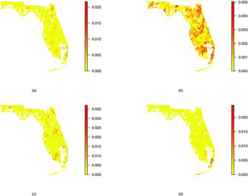
The data considered here consist of 6557 childhood cancer cases over the years 2000–2010. The FAPTP data are deidentified and each case includes information on race (one of African American, Caucasian, other and unknown), gender, age, ZIP code of residence (which are assigned to their corresponding ZCTA), and year of diagnosis. Figure 1 displays the percentage of cancer cases between the years 2000–2010 for each of the 983 ZCTAs in Florida for the four different race categories. African American, Caucasian, other and unknown race constitute approximately 17%, 73%, 2%, and 9% of the cases, respectively.

Figure 1. Percentage of total cancer cases within each ZCTA for (a) African American, (b) Caucasian, (c) other, and (d) unknown race.

In regard to identifying spatial clusters of elevated cancer occurrence (goal (i) above), various approaches are available. A spatial cancer cluster is defined as a spatial region of higher than expected cancer counts. The spatial scan statistic (Kulldorff 1997) and its numerous extensions (Duczmal and Assuncao 2004; Assuncao et al. 2006; Kulldorff et al. 2006; Neill, Moore, and Cooper 2006; Walther 2010) were explicitly designed with spatial data in mind and are indispensable tools for identifying spatial cancer clusters. Intuitively, the spatial scan statistic scans all spatial subregions in the domain and tests if the subregion has an elevated number of cancer incidences compared to surrounding regions.

Rather than focusing on a single spatial cluster, a popular alternative is to map smoothed cancer rates across the spatial domain. Such maps provide a visual graphic of cancer incidence across the entire spatial region that can be compared to other spatial variables to identify spatial factors that explain cancer incidence. Such maps are typically produced using a hierarchical framework (Waller et al. 1997; Lawson 2001, 2008; Zhou and Lawson 2008). The advantage to mapping rates across the entire domain (rather than focusing on smaller subregions individually) is that multiple boundaries indicating regions of rapid change in cancer occurrence can be identified. Identifying such boundaries is often referred to as wombling, boundary analysis, edge detection, or barrier analysis. For such analyses, a “wombling” boundary is a boundary over which a sharp change in the spatial variable occurs. Identifying wombling boundaries is associated with spatial cluster detection because both methods identify spatial regions that are different from surrounding neighbors; hence, each method identifies so called “hot spots” of cancer occurrence.

Detecting wombling boundaries, however, is a difficult statistical problem. Lu and Carlin (2005) detected wombling boundaries using thresholds, but this requires the choice of an arbitrary value as the threshold. Li, Banerjee, and McBean (2011b) used model fit criteria such as the Bayesian information criterion (BIC) to mine various model choices which include (or don’t include) edge effects between neighboring spatial regions. Recent works by Ma and Carlin (2007), Lu et al. (2007), Liang, Banerjee, and Carlin (2009), and Li et al. (2011a) use a Bayesian approach to obtain the posterior probability that a zonal boundary is a wombling boundary. However, Lee and Mitchell (2012) argued that such information is weakly identified by the data alone.

The spatial scan statistic was successfully used by Amin et al. (2010) to identify spatial clusters in the FAPTP data but this analysis seeks to also analyze the covariate information. Furthermore, the majority of model-based wombling techniques are not well suited to simultaneously analyze the spatial and covariate information in the FAPTP data. Hence, these methods are useful for identifying spatial clusters (goal (i) above) but not as useful in associating demographic factors to cancer incidence (goal (ii) above). The problem with not including demographic information in the analysis is displayed in Figure 1 where spatial patterns of cancer occurrence differ by race. Hence, ignoring race could result in identifying different spatial cancer clusters and wombling boundaries than would happen if race were in the model.

The challenge with simultaneously analyzing the spatial and covariate information (e.g., gender, race) is the difference in support between the information. That is, the covariate information is about individual cancer cases (i.e., not aggregated to the ZCTA level) whereas the spatial information is about ZCTAs. Because the covariate information in the FAPTP data is on the individual level rather than the ZCTA level, it is not suited for use within a disease mapping analysis similar to Waller et al. (1997) or Lawson (2008) that would model the FAPTP data on the ZCTA scale. Admittedly, the covariate information in the FAPTP data could be aggregated to the ZCTA level but this may result in ecological confounding (Wakefield and Lyons 2010).

To achieve the above specified goals, this article conducts a model-based wombling analysis of the FAPTP data by treating the data as arising from a marked point pattern with an unknown intensity function and extends previous wombling methodology to the case of a marked point pattern. Specifically, a model based on a marked point pattern is able to simultaneously analyze the spatial features (goal (i) above) and demographic features (goal (ii) above) of cancer incidence. Because both the spatial and mark domains are modeled simultaneously, a wombling analysis is not only able to identify spatial boundaries but also boundaries in the mark domain (e.g., regions of sharp change between ages). The unknown intensity function is estimated using Bayesian methods which allows wombling boundaries to be detected using posterior credible intervals of spatial and covariate parameters (i.e., if the posterior credible interval for the difference in rates across regions does not contain zero then the resulting boundary is a wombling boundary).

The remainder of this article is as follows. Section 2 details the proposed wombling model. Section 3 discusses Bayesian estimation of the wombling model. Section 4 discusses results of fitting the model to the FAPTP data and Section 5 concludes.

2 A MARKED POINT PROCESS MODEL FOR CANCER CASES

2.1 Observation Model

Let be the number of childhood cancer occurrences of race African American, Caucasian, Other, Unknown}, gender Female, Male}, age , in ZCTA , and year . Hence, the total number of cancer cases across the entire spatial and mark domain is given by . Furthermore, define x_i = (r, g, a, z, y)_i as the ith observed childhood cancer case. For this analysis, assume that the number of cases N and the corresponding “marks” {x_i} are both random and follow a marked point process (MPP) over the product space with its corresponding intensity function where is an unknown probability mass function (PMF) on the discrete space and δ > 0 is an unknown constant. In this framework, the random quantities (N, {x_i}) are modeled in a conditional manner where, marginally, N follows a Poisson distribution with and, conditional on N, {x_i}^N_{i = 1} are iid random variables with PMF .

In the proposed MPP framework, the main parameter of interest is the PMF because it determines the behavior of cancer cases over Florida (space) and over the mark domain (e.g., age). To illustrate, the spatial distribution of cancer cases across the ZCTA’s is given by the marginal intensity . Likewise, the distribution of the age of cancer patients is determined by . Hence, estimating can expose interesting features of cancer cases over space and marks.

Traditional disease mapping models are special cases of the MPP model. A traditional disease mapping framework models ZCTA counts N_z using a Poisson distribution with . This traditional model can be seen to be a marginal model under the MPP framework by noticing that μ_z = δλ_z, where is the marginal intensity of ZCTAs. The MPP framework, however, simultaneously models the spatial and nonspatial features of the FAPTP data. In this way, the MPP model is not only a disease map over space but “maps” cancer cases over gender, age, year, and race spaces.

2.2 Intensity Function Model

In the above MPP framework, both δ and are unknown parameters and, hence, need to be modeled statistically. While δ is simply a scalar, is a set of 4 × 2 × 20 × 983 × 11 > 1.7 million parameters that need to be estimated using only the 6557 observed childhood cancer cases in the FAPTP data. As such, simplifying assumptions are required to use the sparse FAPTP data to estimate . Assume that can be factored as, (1) where is the conditional PMF of gender for race r, is the conditional PMF of age for race r, is the conditional PMF of ZCTA for race r, is the marginal PMF of race and is the marginal PMF for year. Equation (1(1) ) assumes that the joint PMF of x = (r, g, a, z, y) can be factored as [x] = [r, g, a, z, y] = [r, g, a, z][y] = [g, a, z∣r][r][y] = [g∣r][a∣r][z∣r][r][y], where [ · ] denotes a general PMF.

Under Equation (1(1) ), the, approximately, 1.7 million dimension parameter space is reduced to (2 + 20 + 983) × 4 + 4 + 11 = 4035 dimensions, which is to be estimated using the 6557 FAPTP observations. However, this reduction in the number of parameters comes at the cost of two key simplifying assumptions. The first key assumption is that the year y is independent (separable) of the remaining marks r, g, a, and z. Intuitively, this assumption means that if there is a factor that increases (or decreases) the number of cancer cases per year, this factor works equally on all genders, age groups, ZCTAs, and races. The second key assumption is that, conditional on race, the marks of gender, age, and ZCTA are independent. In other words, race is sufficient to explain differences in cancer cases among age groups, genders, and ZCTAs. Hence, high risk age groups, genders, and ZCTAs may be different for each race. These two key separability assumptions not only reduce the dimension of the parameter space but help with the sparseness of the data by allowing borrowing of information across years, ages, genders, and ZCTAs.

Justification of the above two key assumptions is as follows. First, independent χ²-tests of association between year y and race r, year and gender g, year and age a, year and ZCTA z had p-values less than 0.001, 0.897, 0.483, and 0.079, respectively. Hence, the only significant association at the 0.05 level is between year and race. On the basis of these p-values, separability of year and the remaining marks seems reasonable (note that because the “other” race category only represented 1.6% of the data, the assumptions for a χ²-test of association between year and race might not hold). In regards to the second assumption, conditional on race, cancer counts are prohibitively small for conducting χ²-tests of association for all but Caucasians. For Caucasians, χ²-tests of association between ZCTA and age, ZCTA and gender, and age and gender had p-values of 0.08, 0.88, and 0.68, respectively. From these tests there may be an interaction between ZCTA and age for Caucasians but, due to lack of significance, modeling z and a separately, conditional on race, is reasonable. Absent evidence to the contrary, this analysis assumes that similar results hold for the other races. Subsequent analyses using more data will need to verify this assumption for the other races.

As mentioned above, represents the spatial intensity (i.e., a spatial map) of cancer cases over the 983 ZCTAs. Building from Waller et al. (1997), let (2) where the normalizing constant ensures because is assumed to be a PMF. The quantity is the proportion of the Florida population of race r residing in ZCTA z, h_z is a vector of covariates (e.g., census demographics) with associated coefficients β_r = (β_r1, …, β_rP)′, ψ_z∣r is a spatially-correlated random effect term used to explain the spatial homogeneities in cancer rates for each race and ϵ_z∣r is an unstructured error term that captures any remaining heterogeneities in cancer rates. This analysis assumes h′_z is a 3 × 1 vector containing the covariates median income, percent of population in poverty, and percent of houses built prior to 1990, but other covariates could certainly be considered.

The weights are taken to be known and derived from the 2010 U.S. census. Under the null hypothesis that cancer rates across ZCTAs are equal, represents an “expected cancer case count” for race r in ZCTA z. The parameter exp {ρ_z∣r} = exp {β_r0 + h′_zβ_r + ψ_z∣r + ϵ_z∣r} is referred to as the “relative risk” of ZCTA z and race r. If ρ_z∣r < 0 then ZCTA z and race r is at a decreased risk whereas ρ_z∣r > 0 indicates an increased risk from the expected count .

2.3 Hyperpriors

As prior distributions, let , , and follow Dirichlet distributions with parameter vectors , , and , where each vector w represents the corresponding distribution in the Florida population according to the 2010 census. For example, represents the distribution of females and males in Florida (e.g., would be the proportion of the Florida population that is female). In the case of , the 2010 census only provided information for ages in 5 year blocks (e.g., 0–4, 5–9, 10–14,15–19). Because of this, is set assuming a uniform distribution of ages within the age group. For example, 23% of the children under the age of 19 in Florida are between the ages 0–4. Hence, the first five elements of that correspond to the weights for ages 0–4 are 0.23/5. The leading constants of 0.01 are precision parameters for the prior Dirichlet distribution. Based on these assumptions, for example, a priori with a corresponding prior variance of . Hence, this is a vague prior specification that allows the data to strongly inform the posterior distribution.

The marginal PMF is likely to be a smooth function of y. That is, if |y₁ − y₂| is small because, a priori, large changes in the number of cancer cases from year to year are not expected. The Dirichlet distribution does not inherently model this smoothness; hence, an alternative prior/model for is needed. Let , where the normalizing constant is chosen to ensure . A prior distribution for is induced by assuming φ_y follows a Gaussian process with mean μ_φ and covariance function . For purposes of this article M_ν( · ∣γ) is assumed to be the Matérn correlation function with smoothness parameter ν and decay γ. A value of 0.35 was chosen so that the resulting Matérn correlation functions matched the empirical lag-1 autocorrelation in the number of cancer cases by year. Finally, vague and were used as prior distributions for μ_φ and σ²_φ, respectively, where denotes the shape-rate parmeterization of the inverse-gamma distribution.

Finally, a prior distribution for is induced by assuming prior distributions for β₀, β_r, {ψ_z∣r}, and ϵ_z∣r. Because ϵ_z∣r represents unstructured heterogeneities, let ϵ_z∣r be iid random variates where for all r and estimated using the data. Furthermore, assume β_r0, …, β_rP are iid random variables a priori for all r. The {ψ_z∣r} represent spatial homogeneities in the intensity function . The most common choice is to assume an intrinsic autoregressive structure for ψ_z∣r (Waller et al. 1997) but, as documented by Hodges and Reich (2010) and Hughes and Haran (2013), this can lead to confounding with the main effects β_r0, …, β_rP. Hence, to avoid this confounding, this analysis follows the approach of Hughes and Haran (2013) by modeling φ_z∣r using basis functions from the corresponding Moran’s operator through a first-order adjacency matrix (i.e., two ZCTAs are neighbors if they share a boundary). Further details are available in Hughes and Haran (2013).

3 STATISTICAL INFERENCE

Let θ represent the set of unknown parameters in the model presented in Section 2. The corresponding MPP likelihood for θ is given by (3) where, from Section 2, is the i cancer case (see Diggle 2003; Møller and Waagepeterson 2004; Liang, Banerjee, and Carlin 2009). From (3(3) ), Bayesian inference proceeds by sampling from the posterior distribution [θ∣N, {x_i}]∝L(θ)[θ], where [θ] represents the joint prior distribution of θ.

This analysis uses a Gibbs sampler to sequentially update , and in a Markov chain Monte Carlo algorithm to obtain 50,000 draws from the posterior distribution after 50,000 iterations of burn-in. Proposals , and were generated from a Dirichlet distribution with parameter c × l where c is a constant controlling the precision and l is the current value of the PMF. For example, let be the value of at the tth iteration of an MCMC algorithm. At each step, a proposal was drawn from the Dirichlet distribution with parameter vector . Using this parameterization, the proposal is centered at the current value and c is tuned to control the mixing of the chain. The PMFs and were updated by updating each of the parameters in (2(2) ) and {φ_y} individually for z = 1, …, 983 and y = 2000, …, 2010. To converge to the correct posterior distributions, proposed values for and were normalized at each iteration. To speed up computation, updating was done in parallel.

Figure 2. Spatial log relative risks ρ_z∣r for (a) African American, (b) Caucasian, (c) Other, and (d) unknown race. The black solid lines indicate a wombling boundary (i.e., regions of high rates of change).

One key aspect of this analysis is to identify regions of dissimilarity. That is, a primary research goal is to identify time periods, spatial regions, and ages that exhibit different cancer rates than surrounding neighbors (i.e., to identify wombling boundaries in the spatial and mark domains). This analysis defines a “wombling boundary” to be a boundary where a corresponding 95% credible interval of the difference in intensity between neighboring regions does not contain zero. For example, a wombling boundary (i.e., a region of rapid change in intensity) exists between years y₁ and y₂ if a 95% central credible interval for does not contain zero. To remove population effects, this analysis determines that a spatial wombling boundary exists between ZCTAs z₁ and z₂ if a 95% credible interval for does not contain zero.

Table 1. ZCTA number for the 10 largest posterior means of ρ_z∣r by race

	Race
Rank	African American	Caucasian	Other	Unknown
1	32,447	32,438	32,814	33,109
2	32,616	32,058	32,686	32,461
3	33,039	32,040	32,827	32,664
4	32,697	33,935	34,669	33,170
5	33,136	32,784	32,204	33,136
6	33,170	33,028	32,714	33,014
7	32,805	33,109	32,934	33,174
8	33,404	32,148	34,956	33,607
9	32,399	32,680	33,544	33,166
10	32,254	32,461	33,331	33,016

Table 2. Posterior summary of the coefficients β₁ (median income; MI), β₂ (percent in poverty; PP), and β₃ (percent of homes built prior to 1990; <1990) for each race

	Race
	African American		Caucasian		Unknown
Covariate (hi)	Mean	95% CI	Mean	95% CI	Mean	95% CI
MI	−0.009	(−0.024, 0.006)	0.003	(−0.002, 0.008)	0.042	(0.024, 0.062)
PP	0.052	(0.030, 0.072)	−0.006	(−0.015, 0.004)	0.052	(0.011, 0.094)
<1990	0.005	(−0.003, 0.013)	−0.001	(−0.003, 0.002)	0.016	(0.003, 0.030)

NOTE: Results for the “other” race category were omitted because the data did not contain enough information to estimate these parameters (95% credible interval widths were very large).

Figure 3. Posterior distribution of the temporal intensity of cancer cases () for y ∈ {2000, …, 2010}. The dashed lines are 95% credible interval limits. The vertical dotted line indicates a wombling boundary between 2005 and 2006.

4 RESULTS

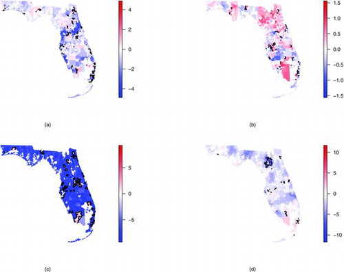
Figure 2 displays the posterior mean for the spatial relative risk parameters ρ_z∣r for . Black solid lines indicate spatial wombling boundaries. Table 1 displays the ZCTA number for the largest 10 posterior means of ρ_z∣r for each race. Comparing each of the subplots, different spatial patterns emerge for each race. Regions of high relative risk are primarily located in the Miami (south-eastern) area for African Americans and results indicate several places with high rates of change (wombling boundaries) in this area. In contrast to African Americans, regions of high relative risk are clustered in the Northern regions for Caucasians (near Jacksonville). These two clusters (north and south) were also found by Amin et al. (2010) but Figure 2 seems to indicate that the Northern cluster is more pronounced for the Caucasian race. Notably, fewer wombling boundaries are found for Caucasians than for African Americans (108 wombling boundaries vs. 206 boundaries were identified for Caucasians vs. African Americans). This difference may be attributable to the sparseness of the data in that small increases in the observed counts (e.g., an increase from 2 to 3 cases) may lead to statistically, but not epidemiologically, significant results. Like African Americans, the wombling boundaries for Caucasians seem to be primarily in the Miami area although there are also several boundaries near Tampa (west-Central). From Figure 2(c) there seems to be very little spatial structure for the “other” race category and the model is only identifying regions where observations occurred (compare with Figure 1(c)). This is likely due to the few number of cases available for this category. For the “unknown” race category, regions of high relative risk seem to be clustered near the southern part of the state with very few wombling boundaries.

Figure 4. Posterior distribution of the age intensity of cancer cases () for (a) African American (b) Caucasian, (c) “other,” and (d) unknown race. The dashed lines are 95% credible interval limits. The vertical dotted lines indicate wombling boundaries.

Table 2 displays the posterior summary for the β_r parameters in (2(2) ). For African Americans, the only significant coefficient is the percent in poverty, suggesting that as the percent in poverty increases, the number of African American cancer cases will also increase. Interestingly, none of the coefficients were significant for the Caucasian race suggesting that any spatial homogeneity is not explained by the included census covariates. In stark contrast, each coefficient was significant for the unknown race category. Because each coefficient was significantly positive, if either median income, percent poverty or percent of homes built prior to 1990 increase, the number of cancer cases will also increase. From these results, it seems that “unknown” is a catchall race category primarily made up of low-income individuals.

Curiously, in Table 2, the coefficient for median income (MI) for the unknown race category is positive. A similar result is found for the Caucasian category wherein the posterior probability that the MI coefficient is greater than zero is 0.91. Perhaps the reason for this is that as median income increases, individuals are more likely to see a doctor which, subsequently, increases the cancer discovery rate. Or, because higher income individuals are more likely to live in cities, these individuals may be more exposed to pollution and other carcinogenic factors. However, these hypotheses are speculative and more research is needed to come to a definitive conclusion.

Figure 3 displays the marginal intensity for y = 2000, …, 2010. Overall, the number of cancer cases is increasing as a function of time. The largest single year increase was between 2005 and 2006, and the analysis found a wombling boundary between these two years. In 2005, there were 570 cases compared to 654 cases in 2006 (a 15% increase). While the temporal trend after 2006 seems to decrease, cancer rates never return to a pre-2005 level.

As displayed in Figure 4, the intensity of childhood cancer cases tends to decrease with age. With the exception of the “other” race category, at least one wombling boundary was found prior to age 5. African American and Caucasian cancer cases both had a wombling boundary between ages 3 and 4 with significantly lower cancer rates after age 4. Both Caucasian and unknown cancer cases saw significantly lower cancer rates after age 0 pointing to a particularly at risk population of new-borns.

Table 3. Posterior mean of gender intensity ()

	Race
	African	Caucasian	Other	Unknown
Gender	American (0.17)	(0.73)	(0.02)	(0.09)
Female	0.45	0.46	0.51	0.47
Male	0.55	0.54	0.49	0.53

NOTE: Numbers next to the race category indicate the posterior mean of the race intensity .

Finally, Table 3 displays the posterior mean of the race and age intensities ( and ). By far, cancer cases seem to be most prevalent among the Caucasian group. However, in the state of Florida, approximately 76% of the population is Caucasian, suggesting that the observed intensity of 0.73 is on par with the rate seen in the population. Likewise, approximately 16% of the Florida population is African American so that the observed intensity of 0.17 is on par with the rate seen in the population. For gender, the observed intensities are also in line with population demographics. That is, for those 19 and under, 52% are male. This value falls within a 95% credible interval for the gender intensity in each category.

5 CONCLUSIONS

This article describes a wombling analysis of FAPTP data of childhood cancer incidence. Specifically, this article modeled FAPTP data as a realization of a marked point process with an unknown intensity function. Subsequently, wombling boundaries on the unknown intensity surface were identified using 95% posterior credible intervals. By fitting the proposed model for the FAPTP data, different wombling boundaries were found for different races. Specifically, regions of high relative risk for African Americans occurred primarily in the Miami area whereas regions of high relative risk for Caucasians occurred in the northern portion of the state.

Because the data were modeled as a marked point pattern, wombling analysis was also performed on the mark domains of age and year. A wombling analysis over the year domain showed that a sharp increase in the rate of childhood cancer incidence occurred between the years 2005–2006. Post-2006 cancer rates never returned to the lower pre-2006 levels. Results also indicated that a sharp decline in cancer incidence occurred between ages 4 and 5 for African Americans and Caucasians.

The results herein are obtained using only 6557 cancer cases over an 11-year time span. This equates to, approximately, 600 cases per year which is, admittedly, rather sparse for estimating separate effects across the different races. The separability assumptions used in Section 2.2 allowed information to be borrowed across years to estimate these random effects but sparse data issues are still present. For example, results regarding covariate effects in Table 2 were excluded for the other race category due to lack of sufficient data to estimate these parameters. While the results herein are valid given the available data and associated modeling assumptions, more data are required to understand the detailed space-time dynamics of cancer incidence.

The methods used in this article to identify spatial cancer clusters via detection of wombling boundaries produces cancer clusters that are not spatially contiguous. In contrast, the spatial scan statistic would produce a spatially contiguous group of ZCTAs that have the highest risk of childhood cancer incidence. While the lack of spatial contiguity may be viewed as a disadvantage, a wombling analysis, by looking at local rates of change, is able to identify any number of ZCTAs that are different relative to their exact neighbors, whereas the spatial scan statistic focuses on finding a global maximum of cancer incidence. Future work could consider extending wombling methodology to produce spatially contiguous regions.

A key assumption in this analysis was the separability of the spatial and temporal intensities. While this assumption was justified for the FAPTP data, such an assumption will certainly not be true for all datasets. Future work with more data could consider a wombling analysis of a nonseparable space-time intensity function and simultaneously identify spatial and temporal wombling boundaries.

References

- Amin, R., Bohnert, A., Holmes, L., Rajasekaran, A., and Assanasen, C. (2010), “Epidemiologic Mapping of Florida Childhood Cancer Clusters,” Pediatric Blood and Cancer, 54, 511–518.
- Assuncao, R., Costa, M., Tavares, A., and Ferreira, F. (2006), “Fast Detection of Arbitrarily Shaped Disease Clusters,” Statistics in Medicine, 25, 723–742.
- Diggle, P. J. (2003), Statistical Analysis of Spatial Point Patterns, London,UK: Arnold.
- Duczmal, L., and Assuncao, R. (2004), “A Simulated Annealing Strategy for the Detection of Arbitrarily Shaped Spatial Clusters,” Computational Statistics and Data Analysis, 45, 269–286.
- Hodges, J. S., and Reich, B. J. (2010), “Adding Spatially-Correlated Errors Can Mess up the Fixed Effect You Love,” The American Statistician, 64, 325–334.
- Hughes, J., and Haran, M. (2013), “Dimension Reduction and Alleviation of Confounding for Spatial Generalized Linear Mixed Models,” Journal of the Royal Statistical Society, 75, 139–159.
- Kulldorff, M. (1997), “A Spatial Scan Statistic,” Communications in Statistics—Theory and Methods, 26, 1481–1496.
- Kulldorff, M., Huang, L., Pickle, L., and Duczmal, L. (2006), “An Elliptic Spatial Scan Statistic,” Statistics in Medicine, 25, 3929–3943.
- Lawson, A. B. (2001), Statistical Methods in Spatial Epidemiology, New York: Wiley.
- ——— (2008), Bayesian Disease Mapping: Hierarchical Modeling in Spatial Epidemiology, Boca Raton, FL: Chapman and Hall/CRC.
- Lee, D., and Mitchell, R. (2012), “Boundary Detection in Disease Mapping Studies,” Biostatistics, 13, 415–426.
- Li, P., Banerjee, S., Hanson, T. E., and McBean, A. M. (2011a), “Nonparametric Hierarchical Modeling for Detecting Boundaries in Areally Referenced Spatial Datasets,” technical Report rr2010-014, Divison of Biostatistics, School of Public Health, University of Minnesota, Twin Cities.
- Li, P., Banerjee, S., and McBean, A. M. (2011b), “Mining Boundary Effects in Areally Referenced Spatial Data Using the Bayesian Information Criterion,” Geoinformatica, 15, 435–454.
- Liang, S., Banerjee, S., and Carlin, B. P. (2009), “Bayesian Wombling for Spatial Point Processes,” Biometrics, 65, 1243–1253.
- Lu, H., and Carlin, B. P. (2005), “Bayesian Areal Wombling for Geographical Boundary Analysis,” Geographical Analysis, 37, 265–285.
- Lu, H., Reilly, C. S., Banerjee, S., and Carlin, B. P. (2007), “Bayesian Areal Wombling via Adjacency Modeling,” Environmental and Ecological Statistics, 14, 433–452.
- Ma, H., and Carlin, B. P. (2007), “Bayesian Multivariate Areal Wombling for Multiple Disease Boundary Analysis,” Bayesian Analysis, 2, 281–302.
- Møller, J., and Waagepeterson, R. P. (2004), Statistical Inference and Simulation for Spatial Point Processes, Boca Raton, FL: Chapman and Hall/CRC Press.
- Neill, D. B., Moore, A. W., and Cooper, G. F. (2006), “A Bayesian Spatial Scan Statistic,” in Advances in Neural Information and Processing Systems 18, eds. Y. Weiss, B. Scholkopf, and J. Platt, . Cambridge, MA: MIT Press, pp. 1003–1010.
- Wakefield, J., and Lyons, H. (2010), “Spatial Aggregation and the Ecological Fallacy,” in Handbook of Spatial Statistics, eds. A. E. Gelfand, P. J. Diggle, M. Fuentes, and P. Guttorp, Boca Raton, FL: Chapman & Hall/CRC, pp. 541–558.
- Waller, L. A., Carlin, B. P., Xia, H., and Gelfand, A. E. (1997), “Hierarchical Spatio-Temporal Mapping of Disease Rates,” Journal of the American Statistical Association, 92, 607–617.
- Walther, G. (2010), “Optimal and Fast Detection of Spatial Clusters With Scan Statistics,” The Annals of Statistics, 38, 1010–1033.
- Zhou, H., and Lawson, A. B. (2008), “Ewma Smoothing and Bayesian Spatial Modeling for Health Surveillance,” Statistics in Medicine, 27, 5907–5928.