Model Uncertainty in Environmental Dose–Response Risk Analysis

Abstract

This article discusses estimation of low-dose “benchmark” points in environmental risk analysis. Focus is on the increasing recognition that model uncertainty and misspecification can drastically affect point estimators and confidence limits built from limited dose–response data, which in turn can lead to imprecise risk assessments with uncertain, even dangerous, policy implications. Some possible remedies are mentioned, including use of parametric model averaging and nonparametric dose–response analysis.

KEY WORDS::

• Benchmark dose
• Environmental risk assessment
• Isotonic dose–response
• Model adequacy
• Model averaging
• Model misspecification
• Multi-model inference

INTRODUCTION

1.1. Background: Environmental Risk Assessment

Regulators and public officials studying the impacts of environmental toxins are called upon to set pollution standards for those agents. The practice is not without its controversies as standards for different toxins can vary, depending on the idealized or realizable nature of the potential exposures (Barnett and O’Hagan 1997). Statistical practice plays a crucial role in the shaping of such standards, where detailed sampling methodology, data acquisition, and statistical analysis are often explicit components (Esterby 2012). Calls have even been made to focus any environmental standard on objective, statistically verifiable formulations (Barnett and Bown 2002; Barnett 2004, chap. 9).

The process of constructing data-based standards for toxic environmental exposures relies heavily on methods of quantitative risk assessment for estimating the risk(s) associated with the particular agent under study. The process of modern risk estimation is often broken down into four fundamental stages (Cogliano 2005): hazard identification, dose–response assessment, exposure assessment, and risk characterization. Important quantitative considerations arise in each of the four stages. For instance, once a dose–response pattern has been established, risk assessors use the consequent statistical estimates to construct statements—and, preferably, valid statistical inferences—on the associated toxicological risk(s). From these, the exposure assessment and risk characterization stages may progress further.

Consider, for example, the analysis of dose–response data in assessment of potential environmental carcinogens: a common design employs a series of doses, x_i (i = 1, …, m), where the x_i's are assumed increasing and the initial dose is typically a zero-valued control: x₁ = 0. Often, observations taken at each x_i are in the form of proportions, Y_i/N_i, where N_i is the number of exposed subjects or objects at the ith dose and Y_i is the number of those subjects that respond to the toxic exposure. This is known as the quantal response data setting, the basic statistical model for which is the binomial: Y_i ∼ indep. Bin (N_i,π_i). Here, π_i is modeled as a function of dose and is often called the risk function: π_i = R(x_i). R(x_i) models the unknown probability that an individual subject will respond at dose x_i, usually through some assigned parametric specification. For instance, the ubiquitous logistic dose–response model is R(x) = 1/(1 + exp{−β₀ − β₁x}), while the similarly popular probit model is R(x) = Φ(β₀ + β₁x), where Φ(·) is the standard normal cumulative distribution function (cdf). The unknown β-parameters and thus the associated risk function are estimated from the data; maximum likelihood (ML) is a favored approach (Piegorsch and Bailer 2005, sec. A.4.3).

1.2. Benchmark Dose Analysis

Once the risk function R(x) has been estimated, a subsequent goal is estimation of the exposure level that produces a low rate of adverse responses in the target population. This involves inversion of the estimated risk function to determine the benchmark dose (BMD) that corresponds to a given, low-level benchmark risk or benchmark response (BMR) (Crump 1984). Rather than focus on R(x), however, it is common with quantal data to define the BMR in terms of a benchmark level of extra risk, R_E(x) = {R(x) − R(0)}/{1 − R(0)}. This adjusts the risk for background or spontaneous effects not associated with exposure to the toxic agent (Piegorsch and Bailer 2005, sec. 4.2). For simplicity, denote the chosen BMR as q ∈ (0,1) and the consequent BMD as ξ_q. The BMD-defining relationship is then simply R_E(ξ_q) = q. The corresponding maximum likelihood estimator (MLE) for the BMD is denoted as .

To account for uncertainty in the estimation process, a 100(1 − α)% lower confidence limit on the true BMD, known as a BMDL and denoted here by , is also calculated (Crump 1995); for example, a simple, one-sided, Wald lower limit employs the asymptotic properties of the MLE to yield (1.1) where z_α = Φ⁻¹(1 − α) and is the large-sample standard error of the MLE. The BMDL has evolved as the target quantity in modern benchmark risk analysis: it is used as a “point of departure” by quantitative risk assessors (Kodell 2009; Izadi Grundy and Bose 2012), who modify it further to account for interspecies extrapolation and other uncertainty factors to establish low-exposure guidelines in practice (Piegorsch and Bailer 2005, sec. 4.4.1).

Table 1. Some common quantal dose–response models in environmental toxicology and carcinogenicity risk assessment, from West et al. (2012)

Model	Code	R(x)	BMD, ξq	Restrictions/notes
Logistic	M1			—
Probit	M2	Φ(β0 + β1x)		QBMR = Φ^−1{q[1 − Φ(β0)] + Φ(β0)}
Quantal-linear	M3	1 − exp { − β0 − β1x}		β0 ≥ 0, β1 ≥ 0
Quantal-quadratic	M4	γ0 + (1 − γ0)(1 − exp { − β1x^2})		0 ≤ γ0 ≤ 1, β1 ≥ 0
Two-stage	M5	1 − exp { − β0 − β1x − β2x^2}		βj ≥ 0, j = 0,1,2
				TBMR = − log(1 − q)
Log-logistic	M6			0 ≤ γ0 ≤ 1, β1 ≥ 0
Log-probit	M7	γ0 + (1 − γ0)Φ(β0 + β1log [x])		0 ≤ γ0 ≤ 1, β1 ≥ 0
Weibull	M8			0 ≤ γ0 ≤ 1, β1 ≥ 1
				WBMR = log{−log(1 − q)}

NOTE: BMD is the benchmark dose. The benchmark response is BMR = q. Φ(·) is the standard normal cdf. The quantal linear (M3) model is also referred to as the “one-stage” or “complementary-log” model, and may equivalently appear as γ₀ + (1 − γ₀)(1 − exp{−β₁x}), where γ₀ = 1 − exp{−β₀}.

1.3. Model Adequacy

A fundamental concern in benchmark analysis is potential sensitivity to/uncertainty with specification of the dose–response function, R(x). Among the wide variety of parametric forms that have been tendered for R(x), many operate well at (higher) doses near the middle range of the observed quantal outcomes; however, the different models can produce wildly different and thus lower limits at small levels of q (Faustman and Bartell 1997; Kang, Kodell, and Chen 2000). In selected instances, the choice for R(x) can be based on biomathematical models that are felt to accurately describe the probability of response, such as the famous multistage model of carcinogenesis (Armitage and Doll 1954; Armitage 1985). Such biologically based dose–response models possess their own levels of uncertainty (Crump et al. 2010), however, and their use is highly selective.

In many cases, little background exists for determining R(x) and its selection is often based on mathematical convenience. Clearly, if a chosen model fails to describe (or even approximate) the true dose–response relationship, estimation and inferences for the BMD can be adversely affected. This short note discusses some recent investigations into the risk-analytic consequences of model uncertainty. Section 2 reviews a recent study by West et al. (2012) on the undesirable effects of model misspecification and model inadequacy in benchmark analysis. Section 3 discusses some possible remedies, using parametric model averaging and nonparametric dose–response analyses. Section 4 illustrates these methods on an example dataset for carcinogenicity assessment, while Section 5 ends with a brief discussion.

2. BENCHMARK DOSE ESTIMATION UNDER MODEL UNCERTAINTY

As noted above, a wide variety of possible parametric forms is available for specifying the dose–response function R(x) in a benchmark analysis. Table 1 lists a series of eight such models popular in toxicological risk assessments with quantal data, including the logit and probit models mentioned above, from a recent study by West et al. (2012). Those authors examined the use of these dose–response models for BMD/BMDL calculation, via a large-scale simulation study. They simulated quantal data from each of the models in Table 1 across a suite of different, increasing, dose–response patterns (very shallow, moderately increasing, broadly increasing, etc.) and with constant per-dose sample sizes of either N = 25, N = 50, N = 100, or N = 1000 subjects/dose.

From their study, West et al. found that model misspecification could drastically affect the coverage performance of the Wald-type BMDL in Equation (1.1)(1.1) . For most of their misspecification pairings—for example, selecting the logistic model (M1) when the data are actually generated from the related log-logistic model (M6)—severe undercoverage for often occurred, and could even spiral down to 0% as sample size increased. Figure 1 illustrates the findings: displayed is a spaghetti plot of the empirical coverage rates as a function of per-dose sample size, N, at the nominal 95% confidence level. Coverages based on correct model specifications are rendered as solid black lines, while those based on misspecified models are dashed gray lines. One sees that when the correct parametric model is employed to build the BMDL, large-sample coverage patterns are stable (as expected; see Wheeler and Bailer 2008), appearing as a block along and above the nominal 95% bar. When the model is misspecified, however, the coverage rates vary wildly, most below the nominal level, and these often tend to drop as N increases. Similar results with nonquantal data have also been observed (Ringblom, Johanson, and Öberg 2014).

Figure 1. Wald-type 95% BMDL coverage for correctly specified (solid black lines) and misspecified (dashed gray lines) models at q = 0.10. (Data from West et al. 2012.) Thick horizontal bar is 95% nominal level.

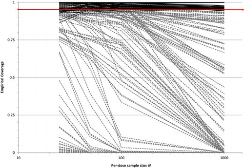
West et al. found no apparent pattern in coverage deterioration among the misspecifications. For example, in Figure 1, the coverage lines for a correct logit (M1) response misspecified with an incorrect probit (M2) model are not greatly different from the correctly specified logit lines; however as mentioned earlier, moving to an incorrectly specified log-logistic (M6) model produces some lines that drop to zero coverage. Such patterns did not remain consistent in any recognizable fashion across the various misspecification pairings.

West et al. also studied model misspecification effects on the extra risk scale, by calculating how far the correct value of R_E() varied from q for various misspecification parings. (Since R_E(ξ_q) is defined as q, one expects R_E() to be less than q, but preferably not too far below it.) While some pairings attained extra risks close to the target level, the authors found that in extreme cases a misspecified R_E() could reach almost eight times above the desired BMR.

Worse still, West et al. found that when employing an information criterion (IC) quantity such as the Akaike information criterion (AIC; see Akaike 1973) to first select a model among the eight candidates, correct selection was more the exception than the rule. For instance, with the commonly seen per-dose sample size of N = 50 subjects/dose, correct selection resulted only about 19% of the time on average across the eight models (West et al. 2012, Table 4). The consequent BMDLs, , constructed under the often-incorrect, AIC-selected model again exhibited unpredictable and unstable coverage patterns.

The implications of these results for those forming policies from risk assessments of toxic agents were clear, if troubling: existing practice of either (i) unequivocally employing a specific dose–response model when there is a possibility of it being misspecified, or (ii) using IC-based selection to first choose the dose–response model, can lead to BMDLs that fail, sometimes utterly, to cover the true BMD. Further adjustment or correction for this model uncertainty must be employed when calculating BMDLs for use in environmental risk analysis.

How to make such adjustments is, of course, a challenge, but one that the statistical community is well suited to address. Some possibilities are described in the next section.

3. ADDRESSING MODEL UNCERTAINTY IN BENCHMARK ANALYSIS

The indications by West et al. (2012) that model misspecification for R(x) can severely undermine proper determination of BMD markers in environmental risk analysis essentially confirmed previous reservations among risk assessors. As noted above, many dose–response functions provide stable fits near the middle range of the observed data. For estimating BMDs and BMDLs at small BMRs, however, one typically operates at doses much closer to zero. There, the different functional forms can produce wildly different benchmark points. These model adequacy issues have been long-recognized concerns in low-dose risk estimation (Glowa 1991; Kang, Kodell, and Chen 2000; Wheeler and Bailer 2013).

Statistical solutions to address issues of model uncertainty/model adequacy for estimating benchmark doses are under active development. Two intriguing strategies are: (i) averaging across an uncertainty class of possible models for R(x) to find model-robust estimates for the risk and for associated quantities such as the BMD or, alternatively, (ii) separating from parametric modeling strategies and adopting model-independent, nonparametric regression techniques. In both cases, recent proposals show promise for overcoming the shortfalls that model uncertainty brings to benchmark analysis. This section describes two examples of these approaches, beginning with the model averaging strategy.

3.1. Multi-Model Inference

In a follow-up article to West et al. (2012), Piegorsch et al. (2013) described a multi-model approach for finding BMDs and BMDLs that appealed to frequentist model averaging (FMA). This was based on a general FMA technology introduced by Buckland et al. (1997). Applied here, the BMD point estimator is taken as a weighted average of individual-model BMDs within a prespecified uncertainty class U_L = M₁, …, M_L of dose–response models M_ℓ, ℓ = 1, …, L. Let be the estimated BMD under the ℓth model. Then, the FMA estimator is the weighted average (3.1)

In (3.1), the ℓth weight is taken as the popular “Akaike” form (3.2) where Δ_ℓ = AIC_ℓ − min{AIC₁, …, AIC_L} and AIC_ℓ is the AIC from the ML fit of the ℓth model M_ℓ. A conservative approximation to the asymptotic standard error of is then constructed, again following Buckland et al. (1997), as (3.3) where is the estimated variance of assuming M_ℓ is correct. (The conservatism enters into the standard error under an assumption that correlations among the estimators approach one. This leads to the simplified expression in (3.3). See Piegorsch et al. (2013) or Buckland et al. (1997) for details.

Of course, many other information criteria could be employed in place of the AIC in Δ_ℓ. These include the Bayesian information criterion, BIC (Schwarz 1978), the “corrected” AIC, AICc (Hurvich and Tsai 1989), or the Kullback information criterion, KIC (Cavanaugh 1999). Piegorsch et al. (2013) studied all these measures, along with original AIC. They found that the FMA-based BMD using AICc was essentially similar to that using AIC, while the KIC- and BIC-based confidence limits were somewhat less stable. (The latter two lost containment of the nominal confidence level and often dropped below it, giving them a “nonprotective” nature not suitable for use in this risk-analytic application; see Section 5.)

Using (3.1) and (3.3), the 100(1 − α)% model-robust FMA BMDL is taken as a simple Wald lower limit, as in (1.1): (3.4)

For the uncertainty class, Piegorsch et al. (2013) employed the collection of L = 8 models in Table 1. Using the same simulation structure from West et al. (2012), they found that the BMDL in (3.4) exhibited very stable coverage characteristics. Empirical coverage rates either achieved or, in a number of cases, conservatively exceeded the nominal level. (The conservatism resulted from the conservative approximation in .) For instance, average per-configuration coverages at the nominal 95% level ranged between 97.1% and 99.8%. The method's ability to hold at or above the nominal level was seen as a plus: the relatively low sample sizes and small numbers of doses employed in most toxicological risk studies can sometimes lead to anticonservative coverage patterns for these sorts of procedures. By contrast, the FMA BMDL in (3.4) almost always produces nominal or somewhat-conservative limits. It provides risk analysts with a model-robust pathway for benchmark inferences that avoids parametric model uncertainty, expanding beyond the collection of single-model parametric forms used in practice. This extended operability allows for improved risk-analytic policy-making in environmental toxicology testing and similar forms of adverse-event risk assessment.

These results suggest that further statistical research into model-averaging strategies for low-dose risk estimation may produce important advances. The FMA construction in (3.1) shares similarities with BMD estimation strategies described by Kang, Kodell, and Chen (2000), Moon et al. (2005), and Bailer, Noble, and Wheeler (2005), although for finding a BMDL it possesses slightly greater computational simplicity. Wheeler and Bailer (2007, 2008) applied a somewhat different tactic and constructed FMA estimates of the entire dose–response curve, producing in effect a model-averaged extra risk, which was then inverted to estimate the BMD for a fixed BMR. They employed bootstrap resampling to find the BMDL, similar to other bootstrap-based FMA approaches given by Faes et al. (2007) and Moon et al. (2013). Also see Ritz, Gerhard, and Hothorn (2013) and Wheeler and Bailer (2013).

Other approaches have applied Bayesian model averaging (BMA) to build the model-robust estimators. Seeded by an early introduction from Whitney and Ryan (1993), BMA BMDs have been applied in a variety of risk-analytic applications (Bailer, Noble, and Wheeler 2005; Morales et al. 2006; Shao and Small 2011, 2012; Shao and Gift 2014). These have particular value if large databases of historical information—typically as historical control data—are available for constructing prior distributions for the Bayesian hierarchy (Shao 2012; Wheeler and Bailer 2012). As with the FMA case, ongoing research into BMA-based BMDLs may provide important insights on how we conduct future, model-robust, quantitative risk assessments and build environmental policies from them.

3.2. Isotonic Regression

One might also eschew the modeling process altogether and default to fully nonparametric estimators for the dose–response. Traditional strategies to avoid parametric model dependencies in low-dose risk analysis have previously relied on the so-called no-observed-adverse-effect level (NOAEL), which does not require specification of R(x). The NOAEL is defined as the highest dose where no statistically significant toxicity is observed. It is usually found via repeated pairwise comparisons between the control group at x₁ = 0 and the various nonzero dose groups. Substantial statistical instabilities have been identified with the use of the NOAEL for risk estimation, however. A NOAEL must by definition correspond to an actual level of the dose under study, thus it is dependent upon the spacing and values of the x_i’s. In fact, if the experiment is badly designed or poorly controlled, excessively high variability can increase the NOAEL. That is, high variability in the response will translate into assertions of low potency (large NOAELs), regardless of the true response effect. Also, a design that allocates too few experimental units to the dose levels may overestimate or even fail to identify an NOAEL. Indeed, it is unclear which parameter(s) of the dose–response relationship these quantities actually estimate. Numerous other concerns have been raised with the use of NOAELs in modern risk assessment, and contemporary analysts recommend against use of this dated technology (Kodell 2009; Öberg 2010; Izadi, Grundy, and Bose 2012). Indeed, Crump (1984) originally suggested the BMD as a more-stable statistical alterative to the NOAEL.

Rather than call upon the outmoded NOAEL, Piegorsch et al. (2014) explored a nonparametric approach using isotonic regression to estimate R_E(x), from which a model-independent BMD could be calculated. Isotonic regression is a general methodology for estimating an unknown response over a series of increasing predictor variables, x_i, using no assumptions on the mean response other than it be ordered in some fashion. For instance, one might assume the response is nondecreasing, as is done below. Then, via clever application of the constraints assumed by the ordering, point estimates can be derived for the underlying mean response; for details, see Silvapulle and Sen (2004, sec. 2.3).

To institute the isotonic regression approach, Piegorsch et al. (2014) assumed the standard binomial model as above, but required only that R(x) be nondecreasing and otherwise unknown. Under these basic assumptions, they isotonized the observed proportions Y_i/N_i, into the nondecreasing sequence via a pool-adjacent-violators (PAV) algorithm (Ayer et al. 1955): (3.5)

From these, empirical estimates of the extra risks were built at each x_i and then connected with a linear interpolating spline to produce an isotonic regression estimator for R_E(x): (3.6) where δ_i(x) = (x − x_i)/(x_i+1 − x_i) and . By inverting this isotonized extra risk at BMR level q, a simple, model-independent estimator for the BMD can be explicitly written as (3.7)

Piegorsch et al. (2012) showed that the estimator in (3.7) was consistent and asymptotically normal, although its large-sample variance was problematic and difficult to estimate. To find a 100(1 − α)% lower confidence bound on ξ_q, denoted as , nonparametric bootstrap resampling with (3.6) was suggested: generate B > 0 bootstrap resamples from the original data and find the bootstrap distribution of . Then, simply take as the αth percentile (the ⌈αB⌉th order statistic) from that bootstrap distribution.

The bootstrapped BMDL based on (3.7) was shown via a simulation study (Piegorsch et al. 2014) to be competitive with the model-robust FMA BMDL described in Section 3.1 when both m and the N_i's are large. For small N_i's and in particular for small m, the nonparametric BMDL could still operate well if the observed dose–response was convex; however, with small numbers of doses, extremely sharp concavity in the dose–response could produce instabilities. In effect, the simple linear interpolator underestimated the concave extra risk function, which led to overestimation of the BMD and hence substandard one-sided lower confidence limits. (Conversely, the linear interpolator overestimated convex dose–response patterns with small numbers of doses, leading to underestimation of the BMD. This engendered some conservatism in the consequent BMDL. As noted in Section 5, however, this may be the lesser of two evils.) Piegorsch et al. (2014) gave an empirical screening criterion that could be used to validate implementation of their isotonic methodology in practical settings. Their introductory foray suggested that further research was called for, to expand the use of robust, nonparametric, and/or semiparametric statistical methods for BMD analysis. These could include more-flexible, adaptive, spline estimators (Bhattacharya and Lin 2010), adjustments for nonmonotone response patterns (Bailer and Oris 2000), or use of semiparametric (Bosch, Wypij, and Ryan 1996; Wheeler and Bailer 2012) and Bayesian nonparametric (Guha et al. 2013) model formulations.

4. EXAMPLE

To illustrate use of the methods from Sections 3.1 and 3.2, consider the following example. Formaldehyde (CH₂O) is a well-known industrial compound, exposure to which can be extensive in a variety of environmental and occupational settings. For instance, concerns over CH₂O contamination of drinking water surfaced in early 2014 after a chemical spill occurred near Charleston, WV. The public outcry led to calls for action on CH₂O pollution among local government officials and policy-makers (Wines 2014).

Table 2. Multi-model benchmark analysis of CH₂O carcinogenicity data in Section 4. Models, M_ℓ, from Table 1. Benchmark response (BMR) set to q = 0.10

Model, Mℓ		AICℓ	wℓ from (3.2)
Logistic, M1	7.2446	35.6226	0.0026	0.0191
Probit, M2	7.1004	31.2633	0.0233	0.1651
Quantal-linear, M3	1.5618	153.7791	5.79 × 10^−29	< 10^−5
Quantal-quadratic, M4	4.0334	61.9964	4.93 × 10^−9	< 10^−5
Two-stage, M5	4.0347	63.9963	—	—
Log-logistic, M6	6.8910	26.0357	0.3175	2.1878
Log-probit, M7	6.9002	24.6198	0.6444	4.4468
Weibull, M8	6.7693	32.5570	0.0122	0.0824

To explore the toxic and carcinogenic potential of the chemical, Schlosser et al. (2003) reported on nasal squamous cell carcinomas observed in laboratory rats after chronic, 2 year, inhalation exposure. Six CH₂O concentrations were studied: x = 0.0, 0.7, 2.0, 6.0, 10.0, and 15.0 ppm. Since intercurrent mortality can occur in such long-term, chronic-exposure studies, the final tumor incidences were adjusted for potential differences in animal survival. The survival-adjusted proportions at each dose were given as Y₁/N₁ = 0/122, Y₂/N₂ = 0/27, Y₃/N₃ = 0/126, Y₄/N₄ = 3/113, Y₅/N₅ = 21/34, and Y₆/N₆ = 150/182. A clearly increasing carcinogenic response was evidenced. Notice that the CH₂O exposure dose, x, is actually a concentration (in ppm) here, and so technically “benchmark concentrations” (BMCs) are computed based on these quantal carcinogenicity data.

Of interest is calculation of the BMC, and more importantly a 95% lower confidence limit, or BMCL, to help inform risk characterization on this potential carcinogen. The analysis here follows that of Piegorsch et al. (2014); it is intended primarily to illustrate the statistical calculations, and not to supersede the larger risk analysis reported by Schlosser et al. (2003) or by any other authors regarding CH₂O carcinogenicity. Following Piegorsch et al. (2014), the BMR is set to the standard value of q = 0.10, and the nominal confidence level is taken as 1−α = 0.95.

4.1. Multi-Model Analysis

To apply the multi-model FMA method in Section 3.1, construct the uncertainty class, U₈, as the L = 8 models in Table 1. Fitting these to the CH₂O carcinogenicity data produces the results given in Table 2. The models yield individual values at q = 0.10 ranging between 1.562 ppm for the quantal-linear model (M3, which exhibits the highest/worst AIC) and 7.245 ppm for the logistic model (M1). The spread here is nontrivial, exhibiting the kind of uncertainty single-parametric model fits can produce with these sorts of data.

Table 2 also gives the intermediate calculations for producing the model-robust, FMA BMC from Equation (3.1)(3.1) , leading to ppm, as seen at lower right. For the model-robust 95% BMCL, similar calculations from Equations (3.3) and (3.4) lead to and ultimately ppm, respectively.

Notice that no weight is listed in Table 2 for the two-stage model (M5). This is an application of “Occam's razor,” as suggested by Wheeler and Bailer (2009) and implemented in Piegorsch et al.'s routines: if a given model's ML fit reduces it to a nested alternative in the uncertainty class, and if the larger model exhibits a higher AIC_q and thus less IC support than the simpler, reduced form, the larger/weaker model is expunged from the averaging process, or equivalently, its weight is set to w_q = 0. This occurs for model M5 with these data: its constrained ML fit (not shown) produces , reducing it to the nested quantal-quadratic model (M4) but with a higher AIC; see Table 2. Thus, the M5 contribution to the model averaged estimator, and to its approximate standard error, is excised from these data.

4.2. Isotonic Regression Analysis

Alternatively, a fully nonparametric benchmark analysis applying the isotonic method from sec. 3.2 appears in Piegorsch et al. (2014). Details can be found therein. Summarizing: concavity in the observed dose–response was assessed and found to be inconsequential in terms of any negative effects on the isotonic estimator. Using (3.7), the model-independent BMC for these data was calculated as ppm. For the 95% BMCL, B = 2000 nonparametric bootstrap resamples were generated. The lower 5th percentile from the resulting bootstrap distribution was given as ppm. The nonparametric and FMA analyses thus give roughly similar benchmark values, and provide comparable points of departure for conducting further risk-analytic calculations on potential formaldehyde carcinogenicity.

By comparison, Schlosser et al. (2003) reported a number of different BMCs and BMCLs, based on a variety of models. For instance, under the log-probit (M7) form they listed a single-model BMC of ppm (consistent with the M7 result in Table 1) and a corresponding BMCL of ppm. Or, for a related form of the Weibull model they gave ppm and ppm.

Schlosser et al. made no adjustments or corrections for multi-model uncertainty in the various, single-model, benchmark points they reported. This was, admittedly, not their goal; however, by applying model-robust strategies such as those discussed herein, concern or confusion over such model uncertainty is ameliorated. These model-robust/model-independent methods free risk assessors from uncertainties about the quality of any parametric assumptions made to support the benchmark computations.

5. DISCUSSION

This missive has reviewed recent considerations on estimation of BMDs in quantitative risk assessment. Ongoing research indicates that statistical calculation of this critical risk-analytic parameter and of its lower confidence limit (BMDL) can be detrimentally affected by model inadequacy and incorrect parametric model selection, to levels not previously realized by the risk assessment community. The potential consequences of such incorrect estimation are nontrivial: a BMDL that overstates its true target BMD quantitatively views large exposures to a potentially hazardous agent as relatively safe. If, in truth, the agent is highly toxic or hazardous, the consequences of such a decision could be severe from a public health and/or environmental safety perspective. (Indeed, this has arguably greater negative impact than incorrectly driving a BMDL too small and consequently imposing strict exposure limitations on an innocuous or weakly toxic agent.) Unless considerable socioeconomic considerations can counterbalance these safety concerns, the error of BMD/BMDL overestimation generates a greater concern for environmental or public health policy when regulating or controlling hazardous agents.

Clearly, all participants in the collaborative risk assessment effort—statisticians, laboratory scientists, risk managers, regulators, and eventual policy-makers—must adopt more flexible data analyses that can adjust for or incorporate model uncertainty. Propitiously, such methods are now being developed by the statistical community, and include robust (parametric) model averaging techniques and model-independent nonparametric analyses. Examples using frequentist model averaging and isotonic nonparametric regression were suggested above, although a more general call can be made for further research and development on this overall theme of model-robust/model-independent estimation in dose–response risk analysis.

REFERENCES

- Akaike, H. (1973), “Information Theory and an Extension of the Maximum Likelihood Principle,” in Proceedings of the Second International Symposium on Information Theory, eds. B.N. Petrov and B. Cs´ki, Budapest: Akademiai Kiado, pp. 267–281.
- Armitage, P. (1985), “Multistage Models of Carcinogenesis,” Environmental Health Perspectives, 63, 195–201.
- Armitage, P., and Doll, R. (1954), “The Age Distribution of Cancer and a Multi-Stage Theory of Carcinogenesis,” British Journal of Cancer, 8, 1–12.
- Ayer, M., Brunk, H.D., Ewing, G.M., Reid, W.T., and Silverman, E. (1955), “An Empirical Distribution Function for Sampling with Incomplete Information,” Annals of Mathematical Statistics, 26, 641–647.
- Bailer, A.J., Noble, R.B., and Wheeler, M.W. (2005), “Model Uncertainty and Risk Estimation for Experimental Studies of Quantal Responses,” Risk Analysis, 25, 291–299.
- Bailer, A.J., and Oris, J.T. (2000), “Defining the Baseline for Inhibition Con-centration Calculations for Hormetic Hazards,” Journal of Applied Toxicology, 20, 121–125.
- Barnett, V. (2004), Environmental Statistics: Methods and Applications, Chichester: Wiley.
- Barnett, V., and Bown, M. (2002), “Statistically Meaningful Standards for Contaminated Sites Using Composite Sampling,” Environmetrics, 13, 1–13.
- Barnett, V., and O’Hagan, A. (1997), Setting Environmental Standards. The Statistical Approach to Handling Uncertainty and Variation, Boca Raton, FL: Chapman & Hall/CRC Press.
- Bhattacharya, R.N., and Lin, L. (2010), “An Adaptive Nonparametric Method in Benchmark Analysis for Bioassay and Environmental Studies,” Statistics and Probability Letters, 80, 1947–1953.
- Bosch, R.J., Wypij, D., and Ryan, L. (1996), “A Semiparametric Approach to Risk Assessment for Quantitative Outcomes,” Risk Analysis, 16, 657–666.
- Buckland, S.T., Burnham, K.P., and Augustin, N.H. (1997), “Model Selection: An Integral Part of Inference,” Biometrics, 53, 603–618.
- Cavanaugh, J.E. (1999), “A Large-Sample Model Selection Criterion Based on Kullback's Symmetric Divergence,” Statistics and Probability Letters, 42, 333–343.
- Cogliano, V.J. (2005), “Principles of Cancer Risk Assessment: The Risk Assessment Paradigm,” in Recent Advances in Quantitative Methods in Cancer and Human Health Risk Assessment, eds. L. Edler and C. Kitsos, Chichester: Wiley, pp. 5–23.
- Crump, K.S. (1984), “A New Method for Determining Allowable Daily Intake,” Fundamental and Applied Toxicology, 4, 854–871.
- ——— (1995), “Calculation of Benchmark Doses from Continuous Data,” Risk Analysis, 15, 79–89.
- Crump, K.S., Chen, C., Chiu, W.A., Louis, T.A., Portier, C.J., Subramaniam, R.P., and White, P.D. (2010), “What Role for Biologically Based Dose-Response Models in Estimating Low-Dose Risk?” Environmental Health Perspectives, 118, 585–588.
- Esterby, S.R. (2012), “Standards, Environmental,” in Encyclopedia of Environmetrics, 6 (2nd ed.), eds. A.H. El-Shaarawi and W.W. Piegorsch, Chichester: Wiley, pp. 2629–2637.
- Faes, C., Aerts, M., Geys, H., and Molenberghs, G. (2007), “Model Averaging Using Fractional Polynomials to Estimate a Safe Level of Exposure,” Risk Analysis, 27, 111–123.
- Faustman, E.M., and Bartell, S.M. (1997), “Review of Noncancer Risk Assessment: Applications of Benchmark Dose Methods,” Human and Ecological Risk Assessment, 3, 893–920.
- Glowa, J.R. (1991), “Dose-Effect Approaches to Risk Assessment,” Neuroscience and Biobehavioral Reviews, 15, 152–158.
- Guha, N., Roy, A., Kopylev, L., Fox, J., Spassova, M., and White, P. (2013), “Nonparametric Bayesian Methods for Benchmark Dose Estimation,” Risk Analysis, 33, 1608–1619.
- Hurvich, C.M., and Tsai, C.-L. (1989), “Regression and Time Series Model Selection in Small Samples,” Biometrika, 76, 297–307.
- Izadi, H., Grundy, J.E., and Bose, R. (2012), “Evaluation of the Benchmark Dose for Point of Departure Determination for a Variety of Chemical Classes in Applied Regulatory Settings,” Risk Analysis, 32, 830–835.
- Kang, S.-H., Kodell, R.L., and Chen, J.J. (2000), “Incorporating Model Uncertainties Along with Data Uncertainties in Microbial Risk Assessment,” Regulatory Toxicology and Pharmacology, 32, 68–72.
- Kodell, R.L. (2009), “Replace the NOAEL and LOAEL with the BMDL01 and BMDL10,” Environmental and Ecological Statistics, 16, 3–12.
- Moon, H., Kim, H.-J., Chen, J.J., and Kodell, R.L. (2005), “Model Averaging Using the Kullback Information Criterion in Estimating Effective Doses for Microbial Infection and Illness,” Risk Analysis, 25, 1147–1159.
- Moon, H., Kim, S.B., Chen, J.J., George, N.I., and Kodell, R.L. (2013), “Model Uncertainty and Model Averaging in the Estimation of Infectious Doses for Microbial Pathogens,” Risk Analysis, 33, 220–231.
- Morales, K.H., Ibrahim, J.G., Chen, C.-J., and Ryan, L.M. (2006), “Bayesian Model Averaging with Applications to Benchmark Dose Estimation for Arsenic in Drinking Water,” Journal of the American Statistical Association, 101, 9–17.
- Öberg, M. (2010), “Benchmark Dose Approaches in Chemical Health Risk Assessment in Relation to Number and Distress of Laboratory Animals,” Regulatory Toxicology and Pharmacology, 58, 451–454.
- Piegorsch, W.W., An, L., Wickens, A.A., West, R.W., Peña, E.A., and Wu, W. (2013), “Information-Theoretic Model-Averaged Benchmark Dose Analysis in Environmental Risk Assessment,” Environmetrics, 24, 143–157.
- Piegorsch, W.W., and Bailer, A.J. (2005), Analyzing Environmental Data, Chichester: Wiley.
- Piegorsch, W.W., Xiong, H., Bhattacharya, R.N., and Lin, L. (2012), “Nonparametric Estimation of Benchmark Doses in Quantitative Risk Analysis,” Environmetrics, 23, 717–728.
- ——— (2014), “Benchmark Dose Analysis Via Nonparametric Regression Modeling,” Risk Analysis, 34, 135–151.
- Ringblom, J., Johanson, G., and Öberg, M. (2014), “Current Modeling Practice May Lead to Falsely High Benchmark Dose Estimates,” Regulatory Toxicology and Pharmacology, 69, 171–177.
- Ritz, C., Gerhard, D., and Hothorn, L.A. (2013), “A Unified Framework for Benchmark Dose Estimation Applied to Mixed Models and Model Averaging,” Statistics in Biopharmaceutical Research, 5, 79–90.
- Schlosser, P.M., Lilly, P.D., Conolly, R.B., Janszen, D.B., and Kimbell, J.S. (2003), “Benchmark Dose Risk Assessment for Formaldehyde Using Airflow Modeling and a Single-Compartment, DNA-Protein Cross-Link Dosimetry Model to Estimate Human Equivalent Doses,” Risk Analysis, 23, 473–487.
- Schwarz, G. (1978), “Estimating the Dimension of a Model,” The Annals of Statistics, 6, 461–464.
- Shao, K. (2012), “A Comparison of Three Methods for Integrating Historical Information for Bayesian Model Averaged Benchmark Dose Estimation,” Environmental Toxicology and Pharmacology, 34, 288–296.
- Shao, K., and Gift, J.S. (2014), “Model Uncertainty and Bayesian Model Averaged Benchmark Dose Estimation for Continuous Data,” Risk Analysis, 34, 101–120.
- Shao, K., and Small, M.J. (2011), “Potential Uncertainty Reduction in Model-Averaged Benchmark Dose Estimates Informed by an Additional Dose Study,” Risk Analysis, 31, 1561–1575.
- ——— (2012), “Statistical Evaluation of Toxicological Experimental Design for Bayesian Model Averaged Benchmark Dose Estimation with Dichotomous Data,” Human and Ecological Risk Assessment, 18, 1096–1119.
- Silvapulle, M.J., and Sen, P.K. (2004), Constrained Statistical Inference: Order, Inequality, and Shape Constraints, New York: Wiley.
- West, R.W., Piegorsch, W.W., Peña, E.A., An, L., Wu, W., Wickens, A.A., Xiong, H., and Chen, W. (2012), “The Impact of Model Uncertainty on Benchmark Dose Estimation,” Environmetrics, 23, 706–716.
- Wheeler, M.W., and Bailer, A.J. (2007), “Properties of Model-Averaged BMDLs: A Study of Model Averaging in Dichotomous Response Risk Estimation,” Risk Analysis, 27, 659–670.
- ——— (2008), “Model Averaging Software for Dichotomous Dose Response Risk Estimation,” Journal of Statistical Software, 26.
- ——— (2009), “Comparing Model Averaging with Other Model Selection Strategies for Benchmark Dose Estimation,” Environmental and Ecological Statistics, 16, 37–51.
- ——— (2012), “Monotonic Bayesian Semiparametric Benchmark Dose Analysis,” Risk Analysis, 32, 1207–1218.
- ——— (2013), “An Empirical Comparison of Low-Dose Extrapolation from Points of Departure (Pod) Compared to Extrapolations Based Upon Methods That Account for Model Uncertainty,” Regulatory Toxicology and Pharmacology, 67, 75–82.
- Whitney, M., and Ryan, L.M. (1993), “Quantifying Dose-Response Uncertainty Using Bayesian Model Averaging” (with discussion), in Uncertainty Modeling in Dose Response: Bench Testing Environmental Toxicity, ed. R.M. Cooke, Chichester: Wiley, pp. 165–196.
- Wines, M. (2014,Tests Said to Find Formaldehyde in West Virginia Tap Water,” New York Times, p. A16.