Identifying Pediatric Cancer Clusters in Florida Using Log-Linear Models and Generalized Lasso Penalties

Abstract

We discuss the identification of pediatric cancer clusters in Florida between 2000 and 2010 using a penalized generalized linear model. More specifically, we introduce a Poisson model for the observed number of cases on each of Florida’s ZIP Code Tabulation Areas (ZCTA) and regularize the associated disease rate estimates using a generalized Lasso penalty. Our analysis suggests the presence of a number of pediatric cancer clusters during the period over study, with the largest ones being located around the cities of Jacksonville, Miami, Cape Coral/Fort Meyers, and Palm Beach.

KEY WORDS::

• Bregman Algorithm
• Fused Lasso
• Disease clustering
• Generalized Lasso
• Log-linear models
• Pediatric cancer
• Poisson regression

1. INTRODUCTION

A recent analysis of pediatric cancer records collected in Florida between 2000 and 2007 described by Amin et al. (2010) identified two possible cancer clusters (one in south Florida and one in northeastern Florida) using the SaTScan^™ software. This article analyzes an updated version of this dataset covering the years between 2000 and 2010 using a penalized generalized linear model (pGLM), reaching similar conclusions.

The National Cancer Institute defines a disease cluster as “the occurrence of a greater than expected number of cases of a particular disease within a group of people, a geographic area, or a period of time.” This definition makes it clear that disease clusters are a purely statistical construct, but provides little guidance about how to identify them. Accordingly, a number of approaches with somewhat distinct goals have been proposed in the literature. Some methods attempt to identify whether the phenomenon of clustering is present in a dataset, but without trying to determine where the clusters are located (see, e.g., Whittemore et al. 1987; Diggle and Chetwynd 1991). Alternatively, some methods are concerned with identifying spatial (and/or temporal) clusters in a dataset in which their presence is not known. Methods based on scan statistics (e.g., Weinstock 1981; Kulldorff 1997; Tango and Takahashi 2005) are examples of such de novo cluster identification. Finally, methods for confirmatory cluster analysis (which Besag and Newell 1991 call focused tests) are concerned with determining whether the rate of disease in a prespecified area (which might contain some putative health hazard) is higher than expected (see, e.g., Stone 1988; Tango 1995; Morton-Jones, Diggle, and Elliott 1999).

Methods for disease clustering can also be classified according to whether they are designed to work with point-referenced or spatially aggregated (aerial) data. In the case of point-referenced data, it is common to distinguish between distance-based methods (Whittemore et al. 1987; Besag and Newell 1991; Tango 1995, among others), which derive tests based on the distribution of the time/distance between locations on which events occurred, and quadrat-based methods (e.g., Openshaw et al. 1987; Kulldorff and Nagarwalla 1995), which study the variability of case counts in certain subsets of the region of interest (called quadrats). In the case of aerial data, frequency tests similar to those used in quadrat-based methods are frequently used (see, e.g., Potthoff and Whittinghill 1966a, 1966b). Bayesian methods for disease clustering in spatially aggregated data have been proposed by Knorr-Held and Raßer (2000), Green and Richardson (2002), Wakefield and Kim (2013), and Anderson, Lee, and Dean (2013). Other recent contributions to the field include the work of Moraga and Montes (2011), who used local indicators of spatial association (LISA) functions, Charras-Garrido et al. (2012), who used a latent discrete Markov random field estimated using an expectation-maximization algorithm, and Heinzl and Tutz (2014), who proposed a clustering approach that uses fused-lasso penalties to estimate the number of clusters. Kulldorff, Tango, and Park (2003), Waller, Hill, and Rudd (2006), and Goujon-Bellec et al. (2011) presented detailed comparisons of various methods for disease clustering.

It is worth noting that the main goals of disease clustering methods are similar but distinct from those of diseases mapping. Typically, disease mapping applications deal with the estimation of smooth covariate-adjusted risk measures, but do not aim at identifying discontinuities in the risk function. On the other hand, the whole point of methods for de novo identification of cancer cluster is to pinpoint such discontinuities. Of course, these two objectives are not necessarily opposed (see, e.g., Knorr-Held and Raßer 2000; Green and Richardson 2002; Anderson, Lee, and Dean 2013), but they are certainly different.

The data we analyze in this article consist of 6558 cases of pediatric cancer occurring in Florida between January 2000 and December 2010. Covariates available for each of the patients include age, race, and sex. We treat age as a categorical variable with four levels (encompassing patients in the ranges of 0–4, 5-9, 10–14, and 15–19 years of age, respectively). On the other hand, race included in principle seven levels: White (4768 patients), Black (1104 patients), Oriental (73 patients), Polynesian (8 patients), Native American (7 patients), More than One Race (20 patients), and Unknown (578 patients). However, since total population estimates are available only for the categories White, Black, and Other, our analysis combines the cases that fall into the Oriental, Polynesian, Native American, More than One Race, and Unknown categories into a single one (Other). Spatio-temporal information for the cases includes the ZIP Code Tabulation Areas (ZCTAs) of residence of the patient as well as the year of diagnosis. However, although the data are (at least in principle) spatio-temporal in nature, we aggregate the data on each ZCTA over time and ignore the temporal component. We take this approach because annual counts on individual ZCTAs tend to be very small and because environmental factors affecting cancer incidence rates are likely to operate over long time scales, making inter-annual fluctuations less important than spatial trends.

Because cases are geolocated according to the ZCTA of residence of the patient, the focus of this article is on techniques that allow us to identify disease clusters on data that has been aggregated over space and time. Hence, the model we propose assumes that the observed number of cases on each of Florida’s ZCTAs follows a Poisson log-linear model in which over-dispersion is captured through ZCTA-specific random effects, which are regularized (or, alternatively, given a prior distribution) through a fused Lasso penalty (Tibshirani et al. 2005; Friedman et al. 2007; Rinaldo et al. 2009; Chen et al. 2012). We focus on a fused lasso prior rather than a more traditional Gaussian conditional autoregressive prior widely used in spatial statistics and disease mapping because the fussed lasso induces sparsity in the point estimates generated by the model. This allows us to carry out de novo identification of cancer clusters while at the same time providing smoothed risk estimates for each of the spatial units, effectively allowing us to treat the hypothesis testing problem as an estimation problem. One-dimensional versions of this model have been used in change-point and hot-spot estimation in genomics (see, e.g., Tibshirani and Wang 2008) but, to the best of our knowledge, the approach we propose here has never been used in the context of disease clustering or disease mapping applications.

The remaining of the article is organized as follows: Section 2 describes our model for cancer cluster detection and discusses some of its properties. Section 3 describes our computational approach to fitting the model, which relies on nontrivial optimization algorithms. Section 4 presents our results for the Florida dataset. Finally, Section 5 discusses some shortcomings of the models, as well as some implications of the results for cancer surveillance in Florida.

2. IDENTIFICATION OF CANCER CLUSTERS IN FLORIDA USING A PENALIZED GENERALIZED LINEAR MODEL

In this section, we describe the statistical models we use to identify cancer clusters in Florida. We start by considering a model in which we ignore the effect of covariates and discuss modeling the (internally standardized) relative risks for each of the ZCTAs with nonzero pediatric population over the whole period over study. We then explain how these models are extended to account for covariates.

We start by discussing some notation. Let y_i and n_i be, respectively, the total observed number of pediatric cancer cases and the total pediatric population on ZCTA i, where i = 1, …, 979 (Florida has a total of 983 ZCTAs, but four of them had no pediatric population (and, of course, no cases) during the period we study. Hence, our analysis involves data from only 979 ZCTAs). The overall disease rate is then simply . We model the total observed number of cases y_i as a Poisson random variable with intensity η_i, , where and φ_i is a random effect (or, alternatively, a frailty term) that captures overdispersion in the data. The value of θ_i = exp {φ_i} represents the excess risk in ZCTA i, so that θ_i > 1 (or, equivalently, φ_i > 0) suggest areas of increased risk. The log-likelihood associated with this model can be written as (1) where and y = (y₁, …, y₉₇₉)^T. Direct maximization of (1(1) ) leads to the trivial estimate . Instead, we propose to maximize a penalized log-likelihood where the term is the so-called fused lasso penalty (Tibshirani et al. 2005; Friedman et al. 2007; Rinaldo et al. 2009) (2) and denotes the sum over all pairs of Florida’s ZCTAs that share a common boundary with each other. Note that this penalty is the combination of two terms, − λγ∑⁹⁷⁹_{i = 1}|φ_i| (which shrinks individual log risks toward zero) and (which shrinks the log risk of a given region toward that of its neighbors, and therefore encourages smoothness in the risk surface). Hence, the parameters λ and γ control the level of similarity in the estimates for neighboring regions. In particular, λ = 0 implies that the frailty terms are independent a priori and the overdispersion in the counts does not follow any spatial pattern, while λ → ∞ leads to a model in which the level of overdispersion is the same in all ZCTAs. Similarly, γ = 0 implies that no shrinkage is applied, while γ → ∞ implies that the excess risk is zero for all ZCTAs.

From a Bayesian perspective, the fused lasso penalty can be motivated as corresponding to a prior of the form, where is the normalizing constant. It is not difficult to show that C(λ, γ) < ∞ as long as γ > 0 (see, e.g., Kyung et al. 2010). Hence, the fused lasso corresponds to a proper prior as long as γ > 0, but improper if γ = 0.

It is constructive to consider the similarities between the fused lasso penalty and conditionally autoregressive (CAR) models widely used to model spatial patterns in aerial data. In particular, intrinsic CAR priors are often defined in terms of the full conditional prior distributions, where W_{i, j} are known weights, W_{i, +} = ∑⁹⁷⁹_{j = 1, j ≠ i}W_{i, j}, and . A common choice is to let W_{i, j} = 1 if i ∼ j and W_{i, j} = 0 otherwise, in which case the joint prior on (φ₁, …, φ₉₇₉)^T can be written as (3) (For a proof, see, e.g., Rue and Held 2005.) Note that the logarithm of the right-hand side of (3(3) ) resembles the form of the fused lasso with γ = 0 and 1/λ = 2τ², except that the absolute value of the differences between neighbors has been replaced by the squared value of such differences. Hence, we can think of the fused lasso with γ > 0 as a proper, heavy tailed alternative to the traditional CAR prior which, in addition to spatial smoothing, induces shrinkage in the disease rates. Furthermore, because double exponential kernels can be represented as scale mixtures of Gaussian kernels (Andrews and Mallows 1974), it can be easily shown that the fused lasso penalty corresponds to the marginal prior distribution induced by a hierarchical Gaussian CAR model.

Although there are substantial similarities between CAR and fused lasso priors, an important difference is that the penalty function is nondifferentiable at points for which φ_i = 0 for any i or for any pair i ∼ i′. Hence, the posterior mode associated with this model (4) is such that the value for groups of adjacent coefficients can be identical to each other and/or be exactly zero, leading to both a segmentation of the state into groups of neighboring ZCTAs, and to a classification of those groups as having or not having a relative risk significantly different from one (and for those groups of ZTCA that have a relative risk significantly different from one, a shrunk estimate of the corresponding relative risk). We exploit this property to define the kth cancer cluster in the sample as a group of adjacent ZCTAs, with positive log-relative risk, that is, as a group of indexes such that for every j = 1, …, m_k we have and for some j′ = 1, …, m_k we have . Hence, maximizing the penalized log-likelihood allows us to treat the problem of simultaneously testing multiple hypotheses as an estimation problem that can be efficiently solved (see Section 3).

The performance of the model depends critically on the value of the penalty parameters λ and γ, which need to be estimated from the data. In this article, we select these two parameters by minimizing Akaike’s information criterion (AIC; Akaike 1974), (5) where represents the equivalent number of parameters associated with λ and γ (in this case, the number of nonzero blocks of coefficients that are obtained when the values of λ and γ are used to compute the penalized estimates in (4(4) ), see Zou et al. 2007; Tibshirani et al. 2012).

A similar formulation can be used to account for the effect of the available covariates (age, race, and sex). In particular, let y_{i, j, k, l} and n_{i, j, k, l} correspond to the number of pediatric cancer cases and the total pediatric population in ZCTA i = 1, …, 979, age group j = 1, …, 4, race k = 1, …, 3, and sex l = 1, 2 and define the average incidence rate for each of these subpopulations as . We model the counts y_{i, j, k, l} by assuming the excess risk in ZCTA i is the same for all subpopulations, that is, we let , where . Under this formulation, covariate-adjusted estimates of the excess risk can be obtained by solving (6)

3. COMPUTATIONAL IMPLEMENTATION

We solve the maximization problems in (4(4) ) and (6(6) ) using a variation of the “split-Bregman” algorithm discussed in Goldstein and Osher (2009). The algorithm is iterative and relies on a second-order Taylor approximation to the Poisson likelihood and on the introduction of two auxiliary vectors u and d that allow us to break the optimization problem into coupled subproblems that are, individually, easy to solve. In the case of (4(4) ), the algorithm takes the following form.

1. Initialize and pick a tuning parameter ξ that controls the rate of convergence of the algorithm.

2. Starting with k = 0 and until convergence, repeat:

   Figure 1. Raw (left) and estimated (right) overall log relative risks for pediatric cancers in Florida.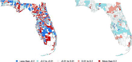

   

   Table 1. Raw incidence rates of pediatric cancer in different covariate-driven subgroups for the four largest clusters identified by our model when there is no adjustment for covariates

   	Incidence (per 100,000 children per year)
   			Age group				Sex		Race
   	Fitted	Raw
   	overall	overall	0–4	5–9	10–14	15–19	Female	Male	Black	White	Other
   North Florida	15.5	18.9	29.0	14.1	15.0	18.1	17.5	20.2	19.1	19.5	11.2
   Miami	16.5	18.1	28.6	14.1	15.0	15.6	18.3	17.9	16.7	14.3	51.3
   Palm Beach	15.3	18.2	28.7	14.6	15.8	14.2	15.8	20.3	20.2	17.7	17.6
   Cape Coral	15.0	18.9	31.4	14.5	15.9	14.4	16.6	21.1	20.8	20.6	5.8
   Florida	–	13.6	21.8	11.1	11.5	10.7	12.8	14.4	13.3	13.4	16.2

   1. Update the parameters of the quadratic approximation to the likelihood function by setting and the vector

   2. Initialize , u^{(k + 1, 0)}, and d^{(k + 1, 0)}.

   3. Starting with l = 0 and until convergence, repeat:

      1. Update the matrix by setting and the vector a^{(k, l)} = (a^{(k, l)}₁, …, a₉₇₉^{(k, l)})^T by setting In the previous expressions, L is an m × 979 matrix (with m representing the number of pairs of ZCTA that are considered neighbors) such that the kth row of L has only two nonzero entries (that correspond to the kth pair of neighbors), which take the values + 1 and − 1.

      2. Initialize .

      3. Starting with s = 0 and until convergence, iterate the following step: where is the soft thresholding operator.

      4. When the previous subiterations have converged, set .

      5. Set , where the thresholding operator is applied componentwise.

      6. Set .

   4. Once this subiteration has converged, set

3. Once these iterations have converged, report as your point estimate for .

Figure 2. Covariate-adjusted log relative risks.

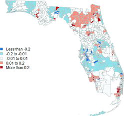
Table 2. Characteristics of the four major clusters under our two models

	Not adjusted for covariates		After adjusting for covariates
	Number of	Total pediatric	Number of	Total pediatric	Number of ZCTAs
	ZCTAs	population	ZCTAs	population	in common
North Florida	91	341,755	98	351,093	90
Miami	73	579,902	70	558,939	70
Cape Coral	32	120,241	26	101,065	26
Palm Beach	24	162,272	25	166,257	24

We present details of the derivation of this algorithm in Appendix A, and note that modifying it to maximize (6(6) ) is straightforward (the only difference being the structure of H and h.) We implemented the iterative thresholding in Step (iii) above using the function crossProdLasso from the R package scout (Witten and Tibshirani 2011). All subiterations were considered to have converged when the relative L² error in the estimate of the vector was less than 10^{− 4}.

To select the hyperparameters λ and γ, we evaluate AIC(λ, γ) over a grid of values of (γ, λ). In particular, we take γ ∈ {0.5, 1, 2}, indicating the ratio of the strength of the pure lasso penalty over that of the fusion penalty is in the range of 50% and 200%. For λ, we first run the path algorithm of Tibshirani et al. (2012) for solving the least-square generalized lasso approximation (A.2(A.2) ) at and then use the output values of λ, at which the solution path changes slope, as the grid for the Poisson generalized lasso.

4. RESULTS

4.1 Relative Risks Without Adjusting for Covariates

Figure 1 shows the raw and estimated overall log relative risks for each of Florida’s ZCTAs before adjusting for race, gender, or ethnicity. These point estimates were generated using the optimal values of and obtained using AIC. By comparing these two maps, we note that our algorithm has the expected effect of smoothing out the raw observations, leading to estimates that involve a large number of ZCTAs with , that is, no increased or reduced relative risks. Our approach also identified 26 possible clusters with elevated overall relative risk involving 274 ZCTAs; some of these clusters had raw risks that were up to four times higher than Florida’s average. Many of these clusters (19 out of the 26) correspond to either isolated ZCTAs or small clusters with only two or three ZTCAs in them. However, the largest clusters (with 91, 73, 32, and 24 ZCTAs and an average at-risk pediatric population of 341,755, 579,902, 120,241 and 162,272 individuals each year) are located in north Florida (the Jacksonville metro area and counties to the West), the Miami metro area, the Cape Coral-Fort Myers metro area and counties to the East, and the county of Palm Beach. The clusters we identify mostly fall within the boundaries of the clusters identified in Figure 1 of Amin et al. (2010); in particular, we seem to find the same small cluster in central Florida that the aforementioned authors identified in their original dataset. However, our clusters tend to be much smaller, suggesting that our methodology allows for more precise identification.

Table 3. Raw incidence rates of pediatric cancer in different covariate-driven subgroups for the four largest clusters identified by our model after adjusting for covariates

	Incidence (per 100,000 children per year)
			Age group				Sex		Race
	Fitted	Raw
	overall	overall	0–4	5–9	10–14	15–19	Female	Male	Black	White	Other
North Florida	15.6	18.9	28.9	14.1	15.1	17.7	17.4	20.2	18.5	19.55	11.5
Miami	16.5	18.0	28.4	13.9	14.9	15.6	18.3	17.7	16.8	14.2	51.2
Palm Beach	15.0	18.0	28.2	14.5	16.2	13.8	15.8	20.1	20.1	17.4	18.0
Cape Coral	15.7	19.1	31.3	14.5	16.2	13.8	16.7	21.3	23.2	20.0	6.2
Florida	–	13.6	21.8	11.1	11.5	10.7	12.8	14.4	13.3	13.4	16.2

Table 1 presents the raw incidence rates of pediatric cancer in different covariate-driven subgroups for these four large clusters, and compares them against the average incidence rate in Florida for the same groups. Note that raw incidence rates in these clusters are between 33% and 39% higher than for Florida as a whole, which is substantial. Also, although the specific patterns vary in the different clusters, disease rates are elevated in almost every subgroup. The main (and somewhat surprising) exception is the racial group “Other” in the Cape Coral-Fort Myers region, which has a very low incidence rate compared to the Florida average for this same group.

Figure 3. Diagnostic residual plots. (a) Deviance residuals against log fitted counts. (b) Half-normal plots of the absolute values of the deviance residuals

4.2 Relative Covariate-Adjusted Risks

Figure 2 presents estimates of the relative risks computed under the covariate-adjusted model in (6(6) ). In this case, the optimal values for the hyperparameters are and , essentially identical to those in Section 4.1. Furthermore, note that this map is very similar to the one presented in the right panel of Figure 1. We now detect 24 possible clusters involving a total of 276 ZCTAs. Table 2 and Appendix A.1(1) present a more detailed comparison of the four major clusters under each of the models. Again, there is substantial agreement between both models, with the cluster under one model being almost completely a subset of the respective cluster under the other.

Similarly to Table 1, Table 3 shows the raw incidence rates of pediatric cancer in different covariate-driven subgroups for the four largest clusters identified by our second model, and compares them against the average incidence rate in Florida for the same groups. As would be expected the results are very similar to those in Section 4.1, with the Miami cluster still exhibiting a particularly large incidence rate among members of the “Other” racial group, and Cape Coral showing a particularly small incidence rate for the same group.

4.3 Validation

4.3.1 Robustness of the Computational Algorithm

To explore the effect of initial values, we initialize the Poisson generalized lasso algorithm at two different and meaningful values. The first is , corresponding to zero log relative risks for all regions, and the second is , corresponding to the observed log relative risks. Because some regions have zero incidents, implying a value of − ∞ for the observed log relative risk, we set the initial log relative risk in these regions equal to the smallest finite value in the sample. The algorithm seems to be robust to the choice of initial values, as the results agree for up to the four decimal place. For the tuning parameter ξ, we explored values between 4 and 40 and found that the performance of the algorithm was quite robust to this choice for both models.

4.3.2 Model Assessment and Goodness of Fit

We assess model fit by inspecting the deviance residuals. The deviance residual for the ith observation is defined as where y_i and are the observed and fitted counts in the region i, and I_{{ · }} is the indicator function. Similarly to linear models, these deviance residuals can be plotted against the logarithm of the fitted values and/or against the quantiles of a half-normal distribution to assess goodness of fit (Neter et al. 1996). Furthermore, we assess the independence in the deviance residuals (and therefore, whether the fused lasso priors capture the spatial structure in the data) by applying Moran’s I test (see, e.g., Banerjee, Gelfand, and Carlin 2004) to the deviance residuals using the moran.test function from the R package spdep (Bivand, Altman, and Anselin 2014).

As an illustration, panel (a) in Figure 3 plots the deviance residuals against the log predicted values for the analysis in Section 4.1. This plot suggests no major problems as most residuals are within 2 in absolute value and there is no obvious relation between the residuals and the predicted values. In the same spirit, panel (b) in Figure 3 shows the half-normal QQ plot of the absolute values the residuals D_i. It shows a couple of points with large residuals, but overall the fit of the model seems appropriate. Finally, the deviance residuals from the pGLM have a Moran I statistic of 0.75 with a p-value of 0.23. In contrast, the D_i’s from the fixed effect intercept-only model have a Moran’s I statistic of 6.36 with a p-value of about 10^{− 10}. This suggests that our pGLM accurately captures the spatial pattern in the data that is missed in the fixed effect model.

Table 4. Performance of three different algorithms under our first simulation scenario. Standard errors are in parentheses

	Proportion of simulations	Average proportion of regions
Method	in which clusters were identified	identified as part of a cluster
pGLM	0.79	0.045 (0.056)
BN (K = 20)	0.97	0.005 (0.003)
BN (K = 200)	0.98	0.020 (0.016)
KN (R = 0.02)	1.00	0.039 (0.014)
KN (R = 0.2)	1.00	0.04 (0.033)

Table 5. Performance of three different algorithms under our second simulation scenario. Standard errors are in parentheses

	Proportion of		Average
	simulations in which no	Average	specificity	Matthews
Method	clusters were identified	sensitivity	coefficient	correlation
pGLM	0	0.62 (0.10)	0.85 (0.06)	0.44 (0.06)
BN (K = 20)	0	0.01 (0.01)	0.99 (0.01)	0.05 (0.04)
BN (K = 200)	0	0.34 (0.08)	0.89 (0.02)	0.24 (0.07)
KN (R = 0.02)	0	0.33 (0.06)	0.91 (0.01)	0.26 (0.05)
KN (R = 0.2)	0	0.69 (0.05)	0.65 (0.05)	0.26 (0.05)

4.3.3 Small-Sample Properties

Since the small-sample properties of the fused lasso as a model selection mechanism are not well understood, we validate our results by undertaking four small simulation studies to assess the probability of a Type I error (i.e., detecting at least one cancer cluster when none is present), Type II error (i.e., not detecting any cluster when at least one is present), as well as the specificity, sensitivity, and Matthews correlation coefficient (or MCC, see Matthews 1975) under different data-generation mechanisms. To provide some context for these results, we also used these simulated scenarios to compare the performance of our model against the two test-based procedures. One is the distance-based method proposed in Besag and Newell (1991) (called BN in the sequel) computed for two different values of its tuning parameter K, which is the number of observed cases for which the number of neighboring regions needed to reach is calculated. We choose K = 20 and K = 200. The other is the quadrat-based likelihood ratio test proposed in Kulldorff and Nagarwalla (1995) (called KN in the sequel) computed for two different values of its tuning parameter R, which is the maximum fraction of the total population used when creating the ball of the cluster. We consider R = 0.02 and R = 0.2. Both BN and KN tests are performed using the opgam function in the R package DCluster (Gómez-Rubio, Ferrándiz-Ferragud, and Lopez-Quílez 2005).

Our first simulation study is carried out under a model in which there are no cancer clusters in Florida. More specifically, we generate 100 datasets y*₁, …, y*₁₀₀, so that the number of cases in ZCTA i = 1, …, 979 for dataset m = 1, …, 100 is given by , where is the average overall pediatric cancer risk observed in Florida between 2000 and 2010. For each of these samples, we computed the number of clusters identified by the model as well as the proportion of regions identified as being part of a cluster by each of the three procedures discussed above (see Table 4 and Figure 4).

Figure 4. Histogram of the number of high relative risk ZCTA () by our penalized generalized linear model on each of the 100 datasets generated under our first simulation scenario.

Our second simulation study involves 100 datasets y*₁, …, y*₁₀₀, where , where correspond to the overall relative risks for the different ZCTAs reported in Section 4.1. Table 5 presents values for the probability of not identifying any cluster in the data, as well as the sensitivity, specificity, and Matthews correlation coefficient associated with each of the three methods for this second scenario.

Table 6. Performance of three different algorithms under our third simulation scenario. Standard errors are in parentheses. MCC is unavailable for pGLM and BN (k = 20) because they detect no clusters at all in some simulated datasets, as this scenario is close to the null scenario of the constant risk

	Proportion of		Average
	simulations in which no	Average	specificity	Matthews
Method	clusters were identified	sensitivity	coefficient	correlation
pGLM	0.22	0.02  (0.03)	0.98  (0.02)	–
BN (k = 20)	0.02	0.006  (0.005)	1.00  (0.004)	–
BN (k = 200)	0	0.03  (0.02)	0.97  (0.02)	0.03 (0.05)
KN (R = 0.02)	0	0.05  (0.02)	0.97  (0.01)	0.04 (0.05)
KN (R = 0.2)	0	0.05  (0.04)	0.96  (0.03)	0.04 (0.05)

Table 7. Performance of three different algorithms under our fourth simulation scenarios. Standard errors are in parentheses

	Proportion of		Average
	simulations in which no	Average	specificity	Matthews
Method	clusters were identified	sensitivity	coefficient	correlation
pGLM	0	0.33 (0.04)	0.90  (0.03)	0.27 (0.06)
BN (k = 20)	0	0.02 (0.01)	1.00  (0.003)	0.06 (0.04)
BN (k = 200)	0	0.15 (0.07)	0.97  (0.02)	0.21 (0.07)
KN (R = 0.02)	0	0.19 (0.06)	0.97  (0.01)	0.24 (0.06)
KN (R = 0.2)	0	0.33 (0.12)	0.87  (0.06)	0.26 (0.08)

As suggested by one of the referees, our third and fourth scenarios deviate from the pGLM model assumption, which assumes that some neighboring regions have exactly the same relative risks. The alternative data generating model is the CAR model. More specifically, let W be a symmetric matrix such that W_{i, j} = 1 if i ∼ j and W_{i, j} = 0 otherwise for i, j = 1, …, 979, and let W_{i, +} = ∑⁹⁷⁹_{j = 1, j ≠ i}W_{i, j}, D_E = diag(W_{1, +}, …, W_{979, +}) and E = (D_W − ρW)/τ². We simulate the log relative risks from a multivariate normal distribution with zero mean and precision matrix E, where the spatial correlation is set to ρ = 0.99. For our third scenario, we use a relatively small value of τ = 0.02, which implies that 95% of the standard deviations of the log relative risks , as can be computed from the diagonal elements of E^{− 1}, are within [0.010, 0.025]. Thus, the simulated log relative risks are largely concentrated around zero and this scenario is close to the null hypothesis where no region has higher than average incidence rates. For our fourth simulation study, we use a moderate value of τ = 0.2, implying that 95% of the standard deviations of the s are within [0.10, 0.25]. The implication is that the simulated log relative risks can be substantially positive and so some neighboring ZCTAs can have high, albeit unequal, log relative risks.

The results presented above suggest that the pGLM has the best overall performance. From Table 4, we see that it has the lowest probability of detecting a false cluster (although that probability is moderately high, suggesting that the model has a moderately large chance of detecting a spurious cluster). On the other hand, Tables 5–7 show that the fussed lasso prior has the highest MCC coefficient. Furthermore, note that in our third scenario the pGLM detects no clusters (regions with positive log relative risks) about 22% of the time but BN and KN almost always detect some clusters. This is probably because the real signal is weak in this case and pGLM aggressively shrinks these weak log relative risks toward zero, but BN and KN impose no shrinkage. On the other hand, in our fourth scenario all models perform poorly, as they tend to identify many small clusters.

5. DISCUSSION

Our analysis of the Florida data suggests the presence of a number of pediatric cancer clusters, with the largest ones being roughly located around the cities of Jacksonville, Miami, Cape Coral/Fort Meyers, and Palm Beach and covering about a quarter of the total pediatric population in the state. We estimate that the risk of pediatric cancers in these regions is at least 30% higher than the state-wide average risk. Importantly, these results seemed to be robust to the inclusion of demographic information. However, our validation using a simulation study suggests that these results must be taken with a grain of salt. Indeed, although our approach has higher sensitivity and specificity and lower Type I error rate than the algorithms we compared it against, it still tends to incorrectly identify at least one cluster in datasets that have been generated under a Poisson model with a constant rate in at least 79% of the cases. In spite of this somewhat negative result, we believe that at least some of the biggest clusters are indeed real because of the high MCC index in our method and the fact that the number of ZCTAs with elevated relative risks in the Florida data is much larger than the numbers we observed when applying our method to data simulated under the null model.

One potential shortcoming of our approach is that overdispersion is captured only by spatial random effects. Although this type of assumption is common in the literature on disease mapping, it can potentially lead to the detection of clusters even if the overdispersion does not follow a well-defined spatial pattern (e.g., if the data arise as independent and identically distributed from a negative binomial distribution). Although the literature on cancer cluster identification is ambivalent about whether all sorts of overdispersion should suggest the presence of clusters or not, we believe that some sort of spatial coherence in the structure of the clusters is desirable. That is the reason why in our discussion of the results we have focused on the four largest clusters identified by our algorithm. A more conservative approach that would deal with this issue would include independent random effects to account for nonspatial structure in the overdispersion in addition to the spatial random effects (see, e.g., Banerjee, Gelfand, and Carlin 2004).

It is worth emphasizing that we did not carry out a full Bayesian analysis of the data and instead focused on providing point estimators based on the posterior mode. We took this approach for two reasons. First, it is important to note that the estimates of the differences in rates are exactly zero only in the posterior mode, neither the posterior mean nor the posterior median are exactly zero under this prior. Since these exact zeros is what allows us to identify disease clusters, and identifying clusters is the main goal of our analysis (rather than creating smooth estimates of the incidence map), fully Bayesian inference is not needed (except as a way to obtain credible intervals for the ZCTA-specific risks, but that is just a secondary goal of our analysis). Second, a fully Bayesian implementation of this model is not quite straightforward. A Gibbs sampler can be constructed using a combination of slice sampling (to deal with the fact that we have a Poisson likelihood, see, e.g., Damien, Wakefield, and Walker 1999) and a data augmentation approach that writes the double exponential prior as a scale mixture of Gaussians (see, e.g., Kyung et al. 2010). However, a sampler of this type mixes poorly. There are ways to improve mixing (e.g., by working directly with the double exponential prior without the data augmentation), but developing the associated theory seemed beyond the scope of an applied article that was meant to be part of a collection focusing on different approaches to analyze a particular dataset. This line of research will be pursued elsewhere.

APPENDIX A: DERIVATION OF THE COMPUTATIONAL ALGORITHM

We derive our algorithm for solving (4(4) ) for a slightly more general model where the log relative risk in region i = 1, …, I, is modeled as a linear function of a set of predictors and we assume a generalized lasso penalty. In this case, the log-likelihood function takes the form (A.1) and the fused lasso penalty (2(2) ) can also be written in a general way as where ||u||₁ = ∑|u_l| denotes the L¹ norm of the vector u, and L is a pre-specified m × p penalty matrix. The random effect model in (1(1) )–(2(2) ) corresponds to the special case of x_i = e_i, where e_i has all entries 0 except that the ith entry equals 1, , and L is a (very sparse) pairwise difference matrix whose rows correspond to pairs of ZCTAs that share a common boundary. Similarly, (6(6) ) can be written in a similar form by extending the sum over ZCTAs in (A.1(A.1) ) to also include sums over all demographic groups.

Recall that the (unpenalized) log-likelihood (A.1(A.1) ) can be optimized using iteratively reweighted least squares (IRLS), that is, by iteratively computing where is obtained by a second-order expansion of (A.1(A.1) ) around the previous iterate , with and

Similarly, we propose to optimize (4(4) ) by iteratively solving (see, e.g., Krishnapuram et al. 2005; Friedman, Hastie, and Tibshirani 2010) (A.2) where each optimization problem in the sequence is accomplished using a variation of the “split-Bregman” algorithm (Goldstein and Osher 2009) described in the next section.

A.1 Solving the Fused Lasso Problem Using the “Split-Bregman” Algorithm

To derive the “split-Bregman” algorithm, introduce a new variable , so that the solution to (A.2(A.2) ) is equivalent to the solution of the following constrained minimization problem, This problem can be solved using an iterative procedure called the Bregman iteration (Bregman 1967; Osher et al. 2005), (A.3) (A.4) where the added L² norm, || · ||₂, of the vector is used to enforce the constraint and ξ is a tuning parameter that controls how fast the constraint is enforced. The final algorithm is obtained by splitting (A.3(A.3) ) into two separate optimization steps, (A.5) (A.6) (A.7)

Note that the solution to (A.6(A.6) ) can be obtained directly using the soft thresholding operator , while the solution to (A.5(A.5) ) can be obtained by applying a coordinate descent algorithm, which reduces to iteratively applying the soft thresholding operator for each component of until convergence.

APPENDIX B: LIST OF ZCTAS IN CANCER CLUSTERS

We list only the ZCTAs in the four main clusters discussed in Sections 4.1 and 4.2. To facilitate comparisons, we separately list the ZCTAs that appear as part of each cluster under both models, and then separately list those that appear under only one of them.

B.2. Palm Beach

					Appear only without	Appear only with
ZCTAs that appear under both models					covariate adjustment	covariate adjustment
33063	33067	33071	33403	33404		33498
33407	33408	33410	33411	33412
33413	33426	33428	33434	33435
33436	33437	33444	33445	33462
33463	33467	33484	33496

B.3. Cape Coral

					Appear only without	Appear only with
ZCTAs that appear under both models					covariate adjustment	covariate adjustment
33901	33903	33904	33905	33907	33440
33908	33909	33912	33914	33916	33471
33917	33919	33920	33922	33924	33930
33935	33936	33950	33955	33956	33931
33957	33971	33972	33990	33991	34134
33993				34142

B.4. Miami

					Appear only without	Appear only with
ZCTAs that appear under both models					covariate adjustment	covariate adjustment
33004	33012	33013	33014	33015	33160
33016	33018	33020	33021	33023	33180
33025	33026	33027	33028	33029	33030
33055	33056	33109	33125	33126
33128	33129	33130	33131	33132
33134	33135	33136	33137	33139
33143	33144	33145	33146	33149
33155	33156	33157	33158	33165
33166	33170	33172	33173	33174
33175	33176	33177	33178	33182
33183	33184	33185	33186	33187
33189	33190	33193	33194	33196
33322	33323	33325	33326	33327
33328	33330	33331	33332	33351

B.5. North Florida

					Appear only without	Appear only with
ZCTAs that appear under both models					covariate adjustment	covariate adjustment
32008	32009	32011	32024	32025	32621	32607
32026	32034	32038	32040	32043		32131
32044	32046	32054	32055	32058		32112
32060	32061	32062	32063	32064		32193
32066	32068	32071	32072	32073		32187
32083	32091	32092	32094	32097		32681
32134	32139	32140	32147	32148		32664
32177	32202	32204	32205	32207		32631
32210	32211	32212	32216	32217
32218	32219	32220	32221	32223
32225	32226	32234	32254	32256
32257	32258	32259	32359	32606
32608	32609	32615	32616	32618
32619	32622	32625	32626	32628
32640	32643	32653	32656	32658
32666	32669	32680	32693	32694
32697	34470	34471	34474	34475
34476	34479	34481	34482	34488

REFERENCES

- Akaike, H. (1974), A New Look at the Statistical Model Identification, IEEE Transactions on Automatic Control, 19, 716–723.
- Amin, R., Bohnert, A., Holmes, L., Rajasekaran, A., Assanasen, C. (2010), Epidemiologic Mapping of Florida Childhood Cancer Clusters, Pediatric Blood & Cancer, 54, 511–518.
- Anderson, C., Lee, D., Dean, M. (2013), Identifying Clusters in Bayesian Disease Mapping,”technical report, arXiv:1311.0660. Available at http://arxiv.org/abs/1311.0660v1
- Andrews, D.F., Mallows, C.L. (1974), Scale Mixtures of Normal Distributions, Journal of the Royal Statistical Society, Series B, 36, 99–102.
- Banerjee, S., Gelfand, A.E., and Carlin, B.P. (2004), Hierarchical Modeling and Analysis For Spatial Data, Boca Raton, FL: CRC Press.
- Besag, J., Newell, J. (1991), The Detection of Clusters in Rare Diseases, Journal of the Royal Statistical Society, Series A, 154, 143–155.
- Bivand, R., Altman, M., Anselin, L. (2014). spdep: Spatial Dependence: Weighting Schemes, Statistics and Models, R package version 0.5-77. Available at http://cran.r-project.org/web/packages/spdep/index.html
- Bregman, L. (1967), The Relaxation Method of Finding the Common Points of Convex Sets and Its Application to the Solution of Problems in Convex Optimization, USSR Computational Mathematics and Mathematical Physics, 7, 200–217.
- Charras-Garrido, M., Abrial, D., De Goër, J., Dachian, S., Peyrard, N. (2012), Classification Method for Disease Risk Mapping Based on Discrete Hidden Markov Random Fields, Biostatistics, 13, 241–255.
- Chen, X., Lin, Q., Kim, S., Carbonell, J.G., Xing, E.P. (2012), Smoothing Proximal Gradient Method for General Structured Sparse Regression, The Annals of Applied Statistics, 6, 719–752.
- Damien, P., Wakefield, J., Walker, S.G. (1999), Gibbs Sampling for Bayesian Non-Conjugate and Hierarchical Models by Using Auxiliary Variables, Journal of the Royal Statistical Society, Series B, 61, 331–344.
- Diggle, P.J., Chetwynd, A.G. (1991), Second-Order Analysis of Spatial Clustering for Inhomogeneous Populations, Biometrics, 47, 1155–1163.
- Friedman, J., Hastie, T., Höfling, H., Tibshirani, R. (2007), Pathwise Coordinate Optimization, The Annals of Applied Statistics, 1, 302–332.
- Friedman, J., Hastie, T., Tibshirani, R. (2010), Regularization Paths for Generalized Linear Models via Coordinate Descent, Journal of Statistical Software, 33, 1–22.
- Goldstein, T., Osher, S. (2009), The Split Bregman Method for l1-Regularized Problems, SIAM Journal of Imaging Sciences, 2, 323–343.
- Gómez-Rubio, V., Ferrándiz-Ferragud, J., Lopez-Quílez, A. (2005), Detecting Clusters of Disease With R, Journal of Geographical Systems, 7, 189–206.
- Goujon-Bellec, S., Demoury, C., Guyot-Goubin, A., Hémon, D., Clavel, J. (2011), Detection of Clusters of a Rare Disease Over a Large Territory: Performance of Cluster Detection Methods, International Journal of Health Geographics, 10, 53.
- Green, P.J., Richardson, S. (2002), Hidden Markov Models and Disease Mapping, Journal of the American Statistical Association, 97, 1055–1070.
- Heinzl, F., Tutz, G. (2014), Clustering in Linear-Mixed Models With a Group Fused Lasso Penalty, Biometrical Journal, 56, 44–68.
- Knorr-Held, L., Raßer, G. (2000), Bayesian Detection of Clusters and Discontinuities in Disease Maps, Biometrics, 56, 13–21.
- Krishnapuram, B., Carin, L., Figueiredo, M.A., Hartemink, A.J. (2005), Sparse Multinomial Logistic Regression: Fast Algorithms and Generalization Bounds, IEEE Transactions on Pattern Analysis and Machine Intelligence, 27, 957–968.
- Kulldorff, M. (1997), A Spatial Scan Statistic, Communications in Statistics—Theory and Methods, 26, 1481–1496.
- Kulldorff, M., Nagarwalla, N. (1995), Spatial Disease Clusters: Detection and Inference, Statistics in Medicine, 14, 799–810.
- Kulldorff, M., Tango, T., Park, P.J. (2003), Power Comparisons for Disease Clustering Tests, Computational Statistics and Data Analysis, 42, 665–684.
- Kyung, M., Gill, J., Ghosh, M., Casella, G. (2010), Penalized Regression, Standard Errors, and Bayesian Lassos, Bayesian Analysis, 5, 369–411.
- Matthews, B.W. (1975), Comparison of the Predicted and Observed Secondary Structure of t4 Phage Lysozyme, Biochimica et Biophysica Acta (BBA)-Protein Structure, 405, 442–451.
- Moraga, P., Montes, F. (2011), Detection of Spatial Disease Clusters With Lisa Functions, Statistics in Medicine, 30, 1057–1071.
- Morton-Jones, T., Diggle, P., Elliott, P. (1999), Investigation of Excess Environmental Risk Around Putative Sources: Stone’s Test With Covariate Adjustment, Statistics in Medicine, 18, 189–197.
- Neter, J., Kutner, M.H., Nachtsheim, C.J., and Wasserman, W. (1996), Applied Linear Statistical Models (Vol. 1), Chicago, IL: Irwin.
- Openshaw, S., Charlton, M., Wymer, C., Craft, A. (1987), A Mark 1 Geographical Analysis Machine for the Automated Analysis of Point Data Sets, International Journal of Geographical Information System, 1, 335–358.
- Osher, S., Burger, M., Goldfarb, D., Xu, J., Yin, W. (2005), An Iterative Regularization Method for Total Variation-Based Image Restoration, Multiscale Modeling and Simulation, 4, 460–489.
- Potthoff, R.F., Whittinghill, M. (1966a), Testing for Homogeneity: I. The Binomial and Multinomial Distributions, Biometrika, 53, 167–182.
- ——— (1966b), Testing for Homogeneity: II. The Poisson Distribution, Biometrika, 183–190.
- Rinaldo, A. (2009), Properties and Refinements of the Fused Lasso, The Annals of Statistics, 37, 2922–2952.
- Rue, H., and Held, L. (2005), Gaussian Markov Random Fields: Theory and Applications, Boca Raton, FL: CRC Press.
- Stone, R.A. (1988), Investigations of Excess Environmental Risks Around Putative Sources: Statistical Problems and a Proposed Test, Statistics in Medicine, 7, 649–660.
- Tango, T. (1995), A Class of Tests for Detecting ‘General’ and ‘Focused’ Clustering of Rare Diseases, Statistics in Medicine, 14, 2323–2334.
- Tango, T., Takahashi, K. (2005), A Flexibly Shaped Spatial Scan Statistic for Detecting Clusters, International Journal of Health Geographics, 4, 11.
- Tibshirani, R., Saunders, M., Rosset, S., Zhu, J., Knight, K. (2005), Sparsity and Smoothness via the Fused Lasso, Journal of the Royal Statistical Society, Series B, 67, 91–108.
- Tibshirani, R., Wang, P. (2008), Spatial Smoothing and Hot Spot Detection for CGH Data Using the Fused Lasso, Biostatistics, 9, 18–29.
- Tibshirani, R.J., Taylor, J., . (2012), Degrees of Freedom in Lasso Problems, The Annals of Statistics, 40, 1198–1232.
- Wakefield, J., Kim, A. (2013), A Bayesian Model for Cluster Detection, Biostatistics, 14, 752–765.
- Waller, L.A., Hill, E.G., Rudd, R.A. (2006), The Geography of Power: Statistical Performance of Tests of Clusters and Clustering in Heterogeneous Populations, Statistics in Medicine, 25, 853–865.
- Weinstock, M.A. (1981), A Generalised Scan Statistic Test for the Detection of Clusters, International Journal of Epidemiology, 10, 289–293.
- Whittemore, A.S., Friend, N., Brown, B.W., Holly, E.A. (1987), A Test to Detect Clusters of Disease, Biometrika, 74, 631–635.
- Witten, D.M., Tibshirani, R. (2011), scout: Implements the Scout Method for Covariance-Regularized Regression, R package version 1.0.3. Available at http://cran.r-project.org/web/packages/scout/index.html
- Zou, H., Hastie, T., Tibshirani, R. (2007), On the “Degrees of Freedom” of the Lasso, The Annals of Statistics, 35, 2173–2192.