Analysis of Battleground State Presidential Polling Performances, 2004–2012

Abstract

This article explores the performance of major political polls as reported on a well-known political website. The presidential elections of 2004, 2008, and 2012 are examined, and polling results for battleground states are compared to the actual margins in each state. These data are combined into an analysis of variance (ANOVA) model and differences in the various polls assessed. No significant differences in polls were found in 2004 or 2008. In contrast, very large differences were found in 2012, and all polls were found to underestimate President Obama’s performance in the battleground states. In addition to individual polling results, a model using the statewide and national polling data from all polls is created. These results are compared to the established polls. We present a possible explanation as to why the polls in the recent (2012) election are all biased toward the Republican side.

• Cell phone
• Elections
• Electoral college
• Predictions sampling.

1. INTRODUCTION

During any presidential election year, considerable attention is paid to political polls. While many members of the media tend to focus on national polls to determine the pulse of the voting public, of more importance in determining the candidate with the electoral edge is evaluating how the candidates are preferred in the so-called “swing states” or “battleground states.” This is a consequence of the Electoral College, which focuses attention on the few states that are both close electorally and carry a significant number of electoral votes. As a result, the election becomes sequestered to a limited number of locales, both from the campaign perspective as well as any dispute that might result from a contested election.

As evidence of this sequestration effect, consider the 2012 presidential campaign. States like Utah and Wyoming were safely in the column of the Republican candidate, Governor Mitt Romney, while Vermont and Hawaii were solidly for President Barack Obama. As a result, little to no campaign funds were spent to woo voters from these states—or from the majority of the remaining. Conversely, the major battleground states of Ohio and Florida had the sums of $ 192 million and $ 119 million, respectively, spent in their states by the two candidates (Wilson 2012). Thus, which candidate voters in Ohio and Florida favor is of more interest when evaluating the likelihood of a candidate winning the election than is that of voters in Wyoming and Vermont. In other words, state polling is more important in predicting the winning candidate than is national polling.

There exist many different polling entities, and often their polls give different estimates of the level of public preference for the presidential candidates. For example, consider the polls associated with Colorado immediately prior to the November 6, 2012, election (Table 1). As a matter of record, President Obama won Colorado by 4.7 points: 51.2% versus 46.5%. These polls gave a wide range of values. Public Policy Polling (PPP) estimated that Obama had a six-point lead in the state, while Rasmussen Reports had Romney as a three-point favorite. Other polls fell between these two extremes. Such variability leaves many people suspicious of polling data. This suspicion was exemplified by a rash of right-leaning pundits and Romney surrogates in the days leading up to the election making bold predictions of a Romney landslide despite having ample polling data that suggested otherwise (Dick Morris, 11/5/12, Fox News, America Live and on the Record; Karl Rove, 11/1/12, The Wall Street Journal; 11/4/12, Swan Hannity, Fox News, The Hannity Report; George Will, 11/4/12, ABC’s This Week; Rush Limbaugh, 11/5/12, The Rush Limbaugh Radio Show). Reportedly, Governor Romney himself was so confident of a win that he only prepared a victory speech for election night (Washington Post 2012b). As Scheiber (2012) of The New Republic reported, internal Romney polling numbers were not consistent with publicly available polls, though inspection of this information does not necessarily lead to a conclusion of a Romney victory.

Table 1 Polling data from six polling firms for Colorado prior to the 2012 Presidential election. In this table, LV refers to “Likely Voters;” MoE, “Margin of Error.” Obama won Colorado by a 4.7 point margin. Source: Real Clear Politics (2014)

Poll	Dates	Sample	MoE	Obama	Romney	Spread
Public Policy Polling	11/3–11/4	1096 LV	3.0	52	46	Obama + 6
WeAskAmerica	10/30–10/30	1246 LV	2.9	50	47	Obama + 3
Denver Post/SurveyUSA	10/28–10/31	695 LV	3.8	47	45	Obama + 2
Rasmussen Reports	10/29–10/29	750 LV	4.0	47	50	Romney + 3
CNN/Opinion Research	10/26–10/31	764 LV	3.5	50	48	Obama + 2
ARG	10/25–10/28	600 LV	4.0	47	48	Romney + 1

Recently, data from political polls have been vindicated as a result of New York Times blogger and creator of the website fivethirtyeight.com, Nate Silver, who uses statistical modeling to predict the results of elections. While he does not provide the specifics of his methods, he is quite detailed on his philosophy and on the sources for his data. His use of multiple polls, down-weighted for age and pollster quality, prediction adjustments for (polling) house effects, and political and social fundamentals in the states does extraordinarily well (Silver 2012, 2014b). His record for the 2012 election was nearly perfect, correctly predicting the presidential outcome in each state, and all but one of the U.S. Senate races (he missed the North Dakota U.S. Senate contest). This accuracy catapulted Silver into the stratosphere of public attention, making him one of the few people to be both a statistician and a pop culture icon. As a result, he has made many appearances on late night television shows, received positive mentions in magazines and news shows, and became a standard bearer for the value of statistics and data. President Obama even mentioned Silver in his Thanksgiving “turkey pardon” address from the White House Rose Garden, joking that he correctly predicted which turkeys would survive (Associated Press 2012).

Also important to this topic is work by Erikson and Wlezien (1999), who used a time series approach for using state polls to predict election results. Jackman (2005) developed a model allowing for pooling political polls to reduce biases observed in individual polls, what is termed “house effects.” Linzer (2013) created a Bayesian model using state polling results to provide dynamic predictions of election results.

This article explores the performances of major political polls as they relate to the true outcomes for the presidential elections of 2004, 2008, and 2012. A model using polling data, both statewide as well as national, is also presented and assessed. Finally, possible explanations as to why the polls have recently been missing the mark are proposed.

2. MOTIVATION

The Centers for Disease Control (Blumberg et al. 2011) estimated that 38% of all American adults, and almost 40% of all households, have cell phone service but no landline, that is, they are “cellphone-only” (CPO) households. This is up from approximately 8% in 2006. In their 2013 report, they also show that this rate is not consistent across the various demographic groups. Those 18–24 are much more likely to be CPO (54%) than those 35–44 (44%), 45–64 (30%) or 65 and over (12%), the poor more than the not-poor (55% to 35%), the metropolitan more than the nonmetropolitan (40% to 32%), and the Northeast less than all other regions combined (27% to 40%).

Under the assumption that voting probability is independent of CPO status, these numbers raise an interesting question for pollsters: Do landline polls need to be adjusted to account for those not in the sampled population?

Keeter et al. (2006) explored this very question. They examined the exit polls of the 2004 election and concluded that there was no need to adjust poll results to account for the CPO voters. Four years later, Pew Research Center (2010a) updated this research for the 2010 midterm elections. It found

In three of four election polls conducted since the spring of this year, estimates from the landline samples alone produced slightly more support for Republican candidates and less support for Democratic candidates, resulting in differences of four to six points in the margin. One poll showed no difference between the landline and combined samples.

Thus, in those 4 years, the effect of CPO households on poll estimates became practically significant. The proportion of adults in cellphone-only households continues to grow. The finding that CPO households tend to be more Democratic and less Republican shows the importance of adjusting poll estimates to reflect this difference (Pew Research Center 2010b).

Exit polls from the 2012 presidential election suggest that this trend is increasing: the 18–29 age group voted 60% for Obama, while only 44% of the 65 and over age group did (Washington Post 2012a). Additionally, the poor were more likely to vote for Obama than the rich (60% to 44%). Thus, for at least these two categorizations, the distribution of cell phones and the support for Obama suggest that Obama supporters were less likely to be contacted by polling firms than were Romney supporters.

If, indeed, Obama supporters were contacted less frequently by polling firms, adjustments could still be made to produce unbiased estimates. Many polling firms use stratified sampling for data collection, which requires them to weight their estimates in each stratum to adjust for known differences between their sample and the target population. In addition to this inverse probability weighting, polling firms may perform additional weighting to adjust for other known factors, such as known biases in the sampling method (Gallup 2015). The problem is that these estimates are only unbiased when the weights used accurately reflect the differences between the sampled population and the population they are trying to describe (Fuller 2009). Thus, while those polling firms not using weights in their estimation process are at risk of producing biased estimates in the presence of cellphone-only households, those polling firms who use incorrect weights are also in danger.

In the next section, we introduce a weighting method designed to estimate state-level candidate support for all 50 states + DC without relying on potentially biased social science theory. A strength of this method is that it uses multiple sources to estimate support, even in the absence of polling data. Its weakness is that it relies on polling data that may themself be biased.

2.1 A Multi-Level Model of Polling

In lieu of relying on a single poll taken at a single point in time, it may be better to aggregate polls from different levels of analysis. This is not a new idea. Silver (2012), Erikson and Wlezien (1999), Jackman (2005), and Linzer (2013), among others, offered models that aggregate polls in some manner. We, as well as Silver (2012) and Linzer (2013), combine support inferred from the national polls, current state-level polls, and the previous estimate of candidate support. However, where Silver (2012) used social science theory and demographics to adjust his estimates and where Linzer (2013) used historic forecasts to predict election-day outcomes, we use only the polling data—both national-level and state-level—and a random effects model to combine those sources of state-level information (Borenstein et al. 2009). Figure 1 provides a schematic of this process.

Figure 1 Schematic diagram of our method to improve the state-level estimation of candidate support using other available data.

Figure 2 A map of the number of polls in each state. States more heavily polled are indicated by a darker shade. The maximum number of polls is 79, which happened in Ohio. There were no polls in Alaska or the District of Columbia. There were two polls in Hawaii. Note the relatively heavy polling of the battleground states. Source: Real Clear Politics (2012).

2.1.1 National Inference

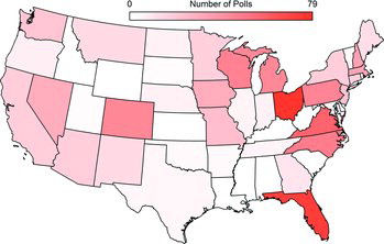
Firms poll nationwide more frequently than for any single state (Figure 2). For instance, between January 4 and November 5, 2012, Real Clear Politics reported 215 national polls, but only 78 for Ohio and 73 for Florida, the two states polled most frequently. Similar conclusions hold for the 2008 election (308 national polls, Ohio and Florida 91 and 83, respectively) and for the 2004 election (219 national polls, Florida and Pennsylvania 69 each).

While the nationwide vote does not elect the president, it does contain information about candidate support at the state level. Regressing state-level popular vote on the nationwide popular vote for presidential elections since 1980 allows one to use the national poll numbers to estimate the state-level candidate support. The amount of information contained in this estimate depends on how well the nation’s popular vote tracks that of the state, that is, on the size of the standard errors. Specifically, a smaller standard error of estimate produces a tighter estimate of the candidate support level in the state. Ohio and Pennsylvania track best; Arkansas and Georgia, worst. National polls give more information about candidate support in Ohio and Pennsylvania than they do in Arkansas and Georgia.

Thus, the level of support for the candidate at each state inferred by his support at the national level calculated using the regression equations is (1) $$p_c={\widehat{\beta }}_0+{\widehat{\beta }}_1{p}_{\mathrm{nat}.}$$(1) Here, p_c is the candidate’s level of support in the state inferred from the national level, p_nat is the level of support for the candidate at the national level, and ${\widehat{\beta }}_0$ and ${\widehat{\beta }}_1$ are the usual ordinary least-square estimates of the intercept and effect. While a logit transformation on the proportions p_nat would not be inappropriate here, the individual model fits as measured by the adjusted R² were not uniformly improved by this adjustment.

Estimated levels of support are of little value without an associated sample size. The effective sample size from this inferred value can be found by noting that the variance of p_c can be obtained from p_c(1 − p_c)/n_c, as well as from direct calculation of the variance of the individual state-level regression Equation (1(1) $$p_c={\widehat{\beta }}_0+{\widehat{\beta }}_1{p}_{\mathrm{nat}.}$$(1) ). Because of the several nonzero covariance terms, the exact formula is complicated. An approximation to the correct value is given by (2) $$V\left(p_c\right)\approx {\text{se}}_1^2{\widehat{\beta }}_1+\frac{p_{\mathrm{nat}}(1-p_{\mathrm{nat}})}{n_c}{\widehat{\beta }}_1^2.$$(2) Setting the two expressions equal gives our estimate for the effective sample size from the inferred value (3) $$n_c\approx \frac{p_c(1-p_c)}{V\left(p_c\right)}.$$(3) Here, V(p_c) is given in Formula (2(2) $$V\left(p_c\right)\approx {\text{se}}_1^2{\widehat{\beta }}_1+\frac{p_{\mathrm{nat}}(1-p_{\mathrm{nat}})}{n_c}{\widehat{\beta }}_1^2.$$(2) ). The national-level estimates, p_nat, must also be estimated. We use an exponential smoother, with rate parameter λ = 1/7, to estimate the candidate support at the national level. That is, if a poll was taken 3 days ago, its weight toward the estimate would be e^{− 3/7} ≈ 0.65. If the poll was taken today, its weight would be e^{− 0/7} = 1.00. We multiply the poll sample sizes by the weight and then estimate the candidate support using this weighted average. We selected this particular weighting function to emphasize that the positions of the American electorate do change through time, but the best current estimate remains the previous estimate.

To see how these processes produce estimates, let us look at two cases, Alabama and Ohio. In the case of Alabama, the regression equation is p_c = 0.4822 + 0.1837p_nat, with se₁ = 0.3547 (and an R² of 0.0473). On July 25, 2012, the estimated Romney support at the national level was 0.4977, with a sample size of 9805. This gives an inferred estimate of Romney support in Alabama of 0.5736, with an effective sample size of only n_c = 11. Thus, there is little information available for Alabama from the national polls. This is primarily due to the large standard error in the regression estimate of the slope.

Contrast this with Ohio, for which the regression equation fits better. Its regression equation is p_c = 0.0603 + 0.9037p_nat, with se₁ = 0.0613 (and an R² of 0.9731). On that same July 25, the inferred support for Romney in Ohio was 0.5101 with an effective sample size of n_c = 73—more than six times higher than Alabama’s.

Notice that the information from national-level polls helps little in estimating candidate support in those states frequently polled, like Ohio. The strength of using this information is in its ability to give some support estimates in states rarely, if ever, polled. Thus, while the national polls altered the estimate for Ohio little, it did affect Alabama’s estimate more.

2.1.2 State Polls

Especially in the battleground states, multiple polls may be completed on the same day. These are combined by simply weighting each by their sample size. (It should be noted that the weighting scheme of Formula (4(4) $$p_s=\frac{\sum p_j{n}_j}{\sum n_j}.$$(4) ) would be incorrect if the polling firms used a sampling design other than simple random sampling, which they tend to do. It would be more correct to weight on the stated margins of error. However, as the margins of error were frequently unavailable in the polls we used, we had to use the simpler formula.) Thus, p_s, our estimated candidate support based on polls in state s is (4) $$p_s=\frac{\sum p_j{n}_j}{\sum n_j}.$$(4)

Here, p_j is the candidate support for poll j and n_j is the sample size of that poll. The effective sample size is n_s = ∑n_j. If there is only one poll in the state on that day, p_s = p and n_s = n, as expected.

Continuing the Ohio example, on October 28, there were two polls. In one, Rasmussen asked 750 likely voters and estimated that 51.02% of the two-party vote supported Romney. In the other, PPP asked 718 likely voters and estimated that 47.96% of the two-party vote supported Romney. Combining these polls gives an estimate of 49.52% for Romney in Ohio.

2.1.3 Previous Estimate

All things being equal, the best estimate of the current level of candidate support today is the estimate of yesterday, that is, if p_{t − 1} is yesterday’s estimated level of candidate support in the state, then today’s estimated level of support is p_t = p_{t − 1}.

While the point estimate is easily determined, the effective sample size is not. The precision of one day’s estimate will decrease with time. However, it is unknown how much. As theory is lacking here, we specify without prejudice that the information decay rate is ξ = 1%; the effective sample size carried forward from yesterday’s estimate is (5) $$n_t=(1-\xi )n_{t-1}=0.99n_{t-1}.$$(5) One interesting result is that success in predicting the winner of a state is rather robust to the choice of information decay rate. Even with a 50% attenuation rate, only two states are miscalled in 2012: Florida, which is even miscalled using 1% attenuation, and West Virginia. The most important effect of increasing the attenuation is to increase the predicted margin of error. As we sought to minimize the margin of error for our estimates, we selected a 1% attenuation. This attenuation produced an average margin of error of 2.13%, compared to 11% for a choice of 50% attenuation.

2.1.4 New Estimate

At this point, we have three pieces of information about the candidate support at the state level: the support inferred from the national level, p_c, the recent state-level polls, p_s, and the candidate’s previous estimated support level in the state, p_t. There are two primary methods (models) for combining several estimates into one: fixed-effects and random-effects. A fixed-effects model assumes that the three sources have the same expected value and that the differences arise from sampling error. A random-effects model assumes the expected values of the three sources are three realizations of a random variable with its own mean, π, and variance, τ² (Borenstein et al. 2009). As the three estimates are not from the same sampled population, we decided that the random-effects model was the more defensible model.

Combining these three sources using a weighted sum produces the state-level support estimate of (6) $$p=\frac{\sum W_k^{*}{p}_k}{\sum W_k^{*}}.$$(6) Here, p_k is the support estimate for each of the three sources, c, s, and t, and W*_k is the associated weight of each. This combining formula (6(6) $$p=\frac{\sum W_k^{*}{p}_k}{\sum W_k^{*}}.$$(6) ) is common to both fixed- and random-effects models. The main difference arises from the meanings of the weights W*_k. Following Borenstein et al. (2009, chap. 12), the intermediate formulas are (7) $$\begin{array}{ccc}\hfill W_k& =& \frac{n_k}{p_k(1-p_k)}\hfill \end{array}$$(7) (8) $$\begin{array}{ccc}\hfill Q& =& \sum W_k{p}_k^2-\frac{{(\sum W_k{p}_k)}^2}{\sum W_k}\hfill \end{array}$$(8) (9) $$\begin{array}{ccc}\hfill C& =& \sum W_k-\frac{\sum W_k^2}{\sum W_k}\hfill \end{array}$$(9) (10) $$\begin{array}{ccc}\hfill T^2& =& \frac{Q-2}{C}\hfill \end{array}$$(10) (11) $$\begin{array}{ccc}\hfill W_k^{*}& =& \frac{1}{V_k+T^2}.\hfill \end{array}$$(11) In these, k represents the three sources of support information, n_k is the effective sample size of that source, p_k is the estimated support level, and V_k is its variance, 1/W_k.

What separates the fixed-effect model from the random-effect model is the allowance for the expected values of the three estimates to be realizations of a random variable with a mean (the true population support level, π) and a variance, τ². Our estimate for this variance is the T² of Formula (10(10) $$\begin{array}{ccc}\hfill T^2& =& \frac{Q-2}{C}\hfill \end{array}$$(10) ), which is the method of moments estimator for τ² (DerSimonian and Laird 1986).

To illustrate the entire process, let us examine the case of Ohio on the eve of the election. The estimated regression equation for Ohio was p_c = 0.0603 + 0.9037p_nat (R² = 0.9731). As our estimate of Romney’s national support on this date was 0.4996, the inferred estimate was p_c = 0.5118 with an effective sample size from this source of n_c = 75. There was but a single poll reported for Ohio that day, which gave Romney p_s = 0.4948 on a sample size of n_s = 1316. Finally, the previous day’s estimates for Romney were p_t = 0.4891 with an effective sample size of n_{t − 1} = 29, 959, which attenuates to n_t = (0.99)29,959 = 29,659.

Combining these together gives raw weight estimates of W_c = 300.167, Ws = 5264.569, and Wt = 118, 692.407 (Formula 7(7) $$\begin{array}{ccc}\hfill W_k& =& \frac{n_k}{p_k(1-p_k)}\hfill \end{array}$$(7) ). Formula (8(8) $$\begin{array}{ccc}\hfill Q& =& \sum W_k{p}_k^2-\frac{{(\sum W_k{p}_k)}^2}{\sum W_k}\hfill \end{array}$$(8) ) gives Q = 0.315 and Formula (9(9) $$\begin{array}{ccc}\hfill C& =& \sum W_k-\frac{\sum W_k^2}{\sum W_k}\hfill \end{array}$$(9) ) gives C = 10, 656.486. This makes our method of moments estimate of the underlying variance (Formula 10(10) $$\begin{array}{ccc}\hfill T^2& =& \frac{Q-2}{C}\hfill \end{array}$$(10) ) T² = 0.000158. As this is negative, we set to T² = 0 (DerSimonian and Laird 1986). As T² is zero, the adjusted weights are just the original weights, W* = (300.167; 5264.569; 118, 692.407). With these weights, we can now apply Formula (6(6) $$p=\frac{\sum W_k^{*}{p}_k}{\sum W_k^{*}}.$$(6) ) to get our unified estimate of Romney’s support in Ohio on November 5, 2012, which is 0.4894 on an effective sample size of 31,050. This gives a 95% confidence interval for Romney’s support in Ohio from 0.4838 to 0.4951. The observed two-party vote share for Romney was 0.4849, which was within the confidence interval and only 0.0045 from the calculated point estimate.

Although we do not use this information for the purposes of this article, this model also provides support estimates in states that had few-to-no polls during the election cycle. In 2012, our sample had three or fewer polls in 17 states, with no polls for eight states (Alaska, Alabama, Delaware, Kansas, Mississippi, South Carolina, West Virginia, and Wyoming). Without using the national polls, the standard errors of support estimates for these 17 states would be extremely large. Using national information reduces these standard errors.

Our model did well in predicting statewide outcomes for the past three presidential elections. In each of these three elections, it incorrectly called only one or two states: Wisconsin in 2004, Indiana and Missouri in 2008, and Florida in 2012. As expected, the model’s worst predictions were for states rarely polled. Thus, it missed Vermont by 6.3% in 2004, Vermont by 7.4% in 2008, and West Virginia by 13.2% in 2012.

However, on average, the model did well in each of the three elections. For all states, the model underestimated Bush in 2004 by an average of 0.65%, Obama in 2008 by 0.38%, and Obama in 2012 by 0.11%. Tables 3 through 5 show this model’s accuracy for just the battleground states.

As expected, the predictions of the model fall within the range of the raw polls. This is because the model essentially uses a weighted average of the state polls to better estimate the true candidate support in each state.

3. METHODS

For the presidential elections of 2004, 2008, and 2012, the states considered to be “battleground states” were determined by those defined as “Toss Up” by the Real Clear Politics (RCP) website (Table 2). Because the voter preference of the candidates can ebb and flow over time, we only used polls closing within 10 days of the election in an effort to afford the polls the best chance of providing a reliable prediction of the election result. In cases in which a firm polled more than once during this time period immediately prior to Election Day, we only considered the latest poll. We used polls that had statewide results listed on the RCP website. For 2012, we also included the internal polling numbers from the Romney campaign for six states (Table 2), as made available by The New Republic (Scheiber 2012).

Table 2 The battleground states, according to Real Clear Politics. Note that the available Romney’s internal numbers are a subset of the 2012 battleground states

2004	2008	2012	Romney 2012 internal
Arkansas	Arizona	Colorado	Colorado	+ 2.5
Colorado	Florida	Florida	Iowa	0.0
Florida	Georgia	Iowa	New Hampshire	+ 2.5
Hawaii	Indiana	Michigan	Pennsylvania	− 3.0
Iowa	Missouri	Nevada	Wisconsin	− 4.0
Maine	Montana	New Hampshire
Michigan	North Carolina	North Carolina
Minnesota	North Dakota	Ohio
Missouri	Ohio	Pennsylvania
Nevada	Virginia	Virginia
New Hampshire		Wisconsin
New Jersey
New Mexico
Ohio
Oregon
Pennsylvania
West Virginia
Wisconsin

For each poll-state combination, the estimated margin of voter preference for the Democratic candidate was recorded, and the difference in this number from the state election result calculated (labeled, for convenience, as DIFF). As an example, consider the November 3, 2012, PPP poll from Colorado that had Obama as a six-point favorite. The difference variable (DIFF) calculated would then be 4.7 (Obama’s actual margin in Colorado) minus 6 to equal − 1.3 (Table 1). Thus, positive values of DIFF would indicate that the poll in question has overestimated the Republican presidential candidate’s performance in that state, while a negative value would point to an overestimate of the Democrat’s.

To assess the overall performance of the polls, separate analyses for each election year were performed. Least square means (adjusted for the lack of balance of polls not occurring in each state) and standard errors for the DIFF values were calculated across states for each poll-election combination. These means serve as overall metrics for the performance of the polls for any given election. The toss-up states used for that particular election were considered to be blocking variables or cofactors. Using these cofactors account for state-to-state variation as well as equalizing the effects of polls not appearing in all states. The analysis of variance procedure compared the means. Also presented are p-values for testing whether a poll’s mean is significantly different from zero. These p-values can be employed as an index of unbiasedness. Large p-values suggest that the bias is insignificant, that the observed mean is not statistically different from zero. Conversely, small p-values would signify that the poll tended to have a bias toward one candidate or the other.

4. RESULTS

4.1 2004 Presidential Election

The states Real Clear Politics considered swing states were Arkansas, Colorado, Florida, Hawaii, Iowa, Maine, Michigan, Minnesota, Missouri, Nevada, New Hampshire, New Jersey, New Mexico, Ohio, Oregon, Pennsylvania, West Virginia, and Wisconsin. Hawaii was not used in this analysis, since no major polls collected data there in the days prior to the election. Table 3 presents the list of the 10 polls assessed in the 2004 presidential election. The polls are listed in order of the bias toward the Democratic candidate, Senator John Kerry. Therefore, for this particular election and for polls that appeared in more than two swing states, SurveyUSA showed the most bias in favor of Kerry, with an average DIFF value of − 3.31; SurveyUSA overestimated Kerry’s performance in swing states by more than 3 points. This is the only poll that had a mean testing significantly different from zero at the nominal 0.05 level of significance.

Table 3 Poll performance numbers in the swing states for the 2004 Presidential election. Seventeen states were used for this analysis.

Polling firm	DIFF Mean	SEM	p-Value
SurveyUSA	−3.31	1.19	<0.01
Research 2000	−2.11	1.81	0.25
ARG	−1.49	1.24	0.23
Rasmussen	−0.65	1.29	0.62
CNN/USAT/Gallup	−0.38	1.63	0.82
FOX News	−0.21	1.79	0.91
Mason-Dixon	0.46	1.29	0.72
LA Times	0.79	2.03	0.70
Strategic Vision (R)	1.71	1.35	0.21
Quinnipiac	2.81	2.43	0.25
Proposed Model	−0.63	1.01	0.54

NOTES: DIFF mean refers to the level of bias associated with a poll, pooled over states and adjusted for the lack of balance of polls appearing in different states, and its estimate of the Democrat’s voter preference. Negative values indicate an overestimate of the Democrat, positive values indicate an overestimate in the favor of the Republican. SEM refers to standard error of the mean estimate, calculated via the ANOVA model. The p-value listed is for testing whether the mean is significantly different from zero

Conversely, the Quinnipiac poll underestimated, on average, Kerry’s support by 2.81 points, making it the most biased poll in the favor of George W. Bush.

For easy reference, the difference values that favor the Democratic candidate are presented in blue font; the Republican, red. The overall p-value from the analysis of variance comparing the means from the 10 polls was 0.20, indicating that there is no significant evidence that these polls differ from each other, adjusted for the cofactor, or blocking factor, STATE.

The proposed model uses all of the polling data and past and present national polls. As such, its estimates are weighted averages of the reported polls. In this case, it had an average DIFF value of − 0.63. Note that since they are not the result of a single poll, its estimates were not included in the analysis to compare the polls.

4.2 2008 Presidential Election

According to Real Clear Politics, the swing states in the 2008 election were Arizona, Florida, Georgia, Indiana, Missouri, Montana, North Carolina, North Dakota, Ohio, and Virginia. Table 4 presents the list of polls that were assessed in the 2008 presidential election. Several of these polls partnered with other entities for data collection for one or more of the states. SurveyUSA frequently partnered with the Downs Center, Rasmussen with FOX News, Mason-Dixon with NBC, and InsiderAdvantage with both Politico and Poll Position. As with the 2004 data, the polls are listed in order of the bias toward the Democratic candidate, Senator Barack Obama.

Table 4 Poll performance numbers in the swing states for the 2008 Presidential election. Ten states were used in this analysis.

Polling firm	DIFF mean	SEM	p-Value
Quinnipiac	−3.37	1.89	0.08
National Journal/FD	−2.19	1.42	0.13
CNN/Time	−1.62	1.21	0.19
Research 2000	−1.21	1.30	0.36
Associated Press/GfK	−1.14	1.90	0.55
Public Policy Polling	−1.10	1.09	0.32
Reuters/Zogby	−0.61	1.21	0.62
ARG	−0.56	1.06	0.60
SurveyUSA	−0.47	1.14	0.68
InsiderAdvantage	0.15	1.59	0.92
Marist	0.19	1.90	0.92
Rasmussen	0.47	1.05	0.66
Mason-Dixon	1.11	1.14	0.33
Strategic Vision (R)	1.54	1.59	0.34
Proposed Model	−0.32	1.00	0.75

NOTES: DIFF refers to the level of bias associated with a poll, pooled over states and adjusted for the lack of balance of polls appearing in different states, and its estimate of the Democrat’s voter preference. Negative values indicate an overestimate of the Democrat, positive values indicate an overestimate in the favor of the Republican. SEM refers to standard error of the mean estimate. The p-value listed is for testing whether the mean is significantly different from zero

The 14 means, when compared in an analysis of variance, do not significantly differ from each other (p = 0.40). This result stands in concert with that of the 2004 election.

Of note is that no polling firm produced results that were significantly different than election-day results, though the Quinnipiac poll did approach significance. Our proposed model gave an estimate of − 0.32, which is near the median of the other estimates, as expected.

4.3 2012 Presidential Election

In the 2004 and 2008 elections cycles, the polling firms tended to produce estimates that were close to the actual results. Furthermore, while some polls overestimated the vote proportion for the Democratic candidate, others did the same for the Republican candidate. The individual biases balanced out. The 2012 election did not follow this pattern. Is this due to idiosyncrasies of the election, or has a substantial shift in the polled electorate taken place?

For 2012, the swing states were Colorado, Florida, Iowa, Michigan, Nevada, New Hampshire, North Carolina, Ohio, Pennsylvania, Virginia, and Wisconsin. Table 5 presents the list of polls that were assessed in the 2012 presidential election.

Table 5 Poll performance numbers in the swing states for the 2012 Presidential election. Eleven states were used in this analysis.

Polling firm	DIFF mean	SEM	p-Value
NBC/WSJ/Marist	0.74  a	0.83	0.42
Public Policy Polling	0.79  a	0.66	0.27
WeAskAmerica	1.38  a	0.83	0.13
SurveyUSA	1.74  a	0.90	0.08
CNN/Opinion Research	2.16  a	1.10	0.07
Gravis Marketing	2.56  a	0.78	<0.01
Romney Internal	4.86  b	0.94	<0.01
Rasmussen	4.95  b	0.83	<0.01
ARG	4.98  b	1.17	<0.01
Proposed Model	2.20	0.71	<0.01

NOTES: DIFF refers to the level of bias associated with a poll, pooled over states and adjusted for the lack of balance of polls appearing in different states, and its estimate of the Democrat’s voter preference. Negative values indicate an overestimate of the Democrat, positive values indicate an overestimate in the favor of the Republican. SEM refers to standard error of the mean estimate. The p-value listed is for testing whether the mean is significantly different from zero. Two means with the same letter are not significantly different with the use of protected least significant difference comparisons at the 0.05 level of significance (Tukey 1949)

Figure 3 Comparison of the DIFF mean values from the three polling firms common to all three elections, as well as for our model. The intervals are 95% confidence intervals. Note that only the SurveyUSA DIFF value was not significantly different from zero in the 2012 election.

Figure 4 Map of the estimated prevalence of cellphone-only adults in the United States by state in 2009. Darker colors indicate a higher percentage of the adult population living without land lines. Values range from 11.4% of the adult population in cellphone-only households in New Jersey to 33.5% in Arkansas. Source: Blumberg et al. (2011).

Figure 5 A scatterplot of the bias observed in the Romney internal poll for the 2012 presidential election against the percentage of cellphone-only adults in the five swing states polled (Colorado, Iowa, New Hampshire, Pennsylvania, and Wisconsin). The overall effect (adjusted for poll differences) was β₁ = 0.46 (p = 0.005). Sources: Blumberg et al. (2011) and Scheiber (2012).

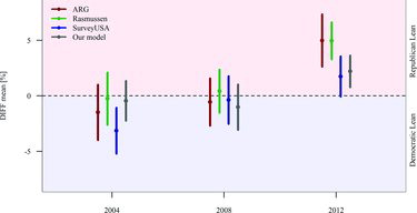
Note that four of the nine polls had mean values that tested significantly different from zero, and did so convincingly with p-values that were less 0.01, indicating significant underestimation of President Obama’s voter preference in the swing states. Also worth noting is that all of the polls in question underestimated Obama’s performance on average. The proposed model, as a result of all of the polls underestimating Obama’s performance, also gave an average estimate that fell short of Obama’s true support.

It is interesting that the nine polling firms fall into two neat categories in terms of how they missed the election results. Rasmussen and ARG both overestimated Romney’s vote share significantly more than any of the other polling firms. The remaining size polling firms, while they did overestimate Romney’s support in the population, they did so much less than the first group. In other words, there may be substance in referring to certain polling firms as either “left-leaning” or “right-leaning.”

Note, however, that this observation depends on which election. In 2008, none of the polling firms differed significantly. In 2004, Rasmussen and ARG were both “left-leaning” firms, especially with respect to Strategic Vision and Quinnipiac University.

5. DISCUSSION

Inspecting Tables 3 through 5 yields some interesting conclusions regarding the polls and how they may have changed over the past three presidential elections. Table 3 shows that both Rasmussen and FOX News performed well in 2004, both showing small bias numbers related to the other polls. In 2008, Rasmussen also showed results very consistent with the election results for the battleground states in which they polled (Table 4). This might come as a surprise to some who think of both entities as typically right-leaning.

However, those who embrace this idea of biasness from these firms could have their suspicions confirmed when looking at the 2012 polling averages (Table 5). FOX News, though still conducting public polls, failed to make our analysis in either 2008 or 2012 due to a lack of available data near Election Day. Rasmussen, on the other hand, showed a heavy bias toward GOP candidate Mitt Romney, missing the actual election results in those battleground states by an average of nearly five percentage points. Is this indicative of a trend for Rasmussen to lean toward the right, or was 2012 just an outlier?

One also has to wonder why the three polls, ARG, Rasmussen, and Romney’s internal numbers, were so different from the remaining polls. Was there a difference in sampling methodology that created this chasm? Simply being different from the other polls is not cause for concern, but being different and inaccurate is problematic.

Our model performed well in 2004 and 2008, which is expected since there were polls that favored the Republican candidate and polls that favored the Democratic candidate in these elections. When combining these polls into one model, the different biases tend to have a cancellation effect. On the other hand, in 2012 all of the polls examined overestimated Romney’s support, so our model likewise overestimated that support. In fact, of the 11 battleground states, our model missed by more than our margin of error four times (Colorado, Michigan, Nevada, and New Hampshire), with our estimate of Michigan missing by approximately two margins of error. Our best prediction was for North Carolina, where we predicted Romney winning with 51.05%; he won with 51.11%.

One approach that should be considered in modeling future presidential elections is to down-weight polls that showed significant bias, as measured by our ANOVA model and the p-values associated with the mean estimates. This is what Silver (2014a) does, although his methodology for weighting pollsters is based on a different measure of bias. These models that are based only on certain polling information would be beneficial only under the assumption that polls that display bias in 2012 would also do so in 2016. This is not an easy assumption to embrace, since the consistency of the polls from election to election is not supported by these data. Furthermore, Silver (2014b) concluded that pollster ratings were not a practically significant factor in predictions.

The fact that all of the polls listed for 2012 missed the election in the same direction (see Table 5 and Figure 3) is intriguing. Conversely, inspection of Tables 3 and 4 shows that some polls are painted red (overestimated the Republican candidate), while others are blue (overestimated the Democratic candidate). This is not true for 2012. What happened?

One explanation is that the election “broke” for Obama. In other words, there were many voters in the swing states that either changed or made up their minds right before the election, eluding detection from the preelection polls. Many pundits speak of elections breaking in this way, and perhaps this was what the Romney camp was confident would happen (albeit, in the other direction). Perhaps Obama’s leadership exhibited in the aftermath of Superstorm Sandy affected these last-minute voters.

5.1 Cellphone-Only Voters

Regardless, one must also worry that this bias, seen across all polls, might have roots in outdated and possibly flawed sampling methodology. Could the polls be underestimating a certain segment of the voting population that tends to vote Democratic?

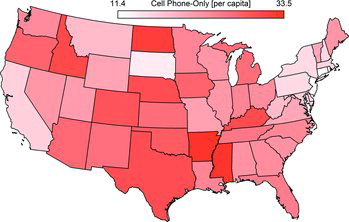
Our cellphone culture may be an explanation (Figure 4). Polling of landlines is easier and less costly. To protect cell phone user from paying for unsolicited calls, pollers must dial cellphone numbers manually. Conversely, landlines can be contacted via computer-generated dialing (Samuelson 2012). However, increasingly U.S. citizens, and therefore, potential voters, are relying solely on cellphones and not maintaining landlines in their homes. According to Marketing Charts (2012), the percentage of households that solely relied on wireless phones from 2008 to 2011 increased from 17.5% to 34.0%. During this same period, the percentage of households with a landline decreased from 79.1% to 63.6%. According to Mokrzycki, Keeter, and Kennedy (2009), face-to-face exit polls from the 2008 election suggest that differences in voting preferences in landline and cellphone-only voters exist, and this difference is not completely attributable to age. Even for older voters, the voting preference difference between these two groups is substantial. Pew Research Center (2010a) concluded:

Cell-only adults are demographically and politically different from those who live in landline households; as a result, election polls that rely only on landline samples may be biased. Although some survey organizations now include cell phones in their samples, many—including virtually all of the automated polls—do not include interviews with people on their cell phones.

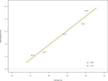
In an effort to assess the relationship between cellphones and polling bias, we created a model regressing the bias variable DIFF on the percentage of cellphone-only for the swing states we used in the analysis of the 2012 election households (Blumberg et al. 2011). The regression coefficient is adjusted for poll, since the observations contained in the regression are not independent and poll-to-poll variation will account for much of the error observed. Figure 5 illustrates this relationship for the five battleground states Romney used for his internal polling.

The relationship of bias to cellphone-only percentage yields an effect estimate of 0.46 (p = 0.005). This means a one percentage point bias toward Romney is observed for every two-percentage increase in cellphone-only percentage, on average.

Do political sampling methodologies need to be enhanced or developed to account for this potential source of bias? Tucker, Brick, and Meekins (2007) suggested that weighting could be used to account for the under-representation of cellphone-only respondents in a telephone survey, but applying their methodology in political polling settings appears to be difficult. Samuelson (2012) suggested that no real solution currently exists to address this problem.

6. CONCLUSION

It is important for anyone assessing the future outcome of an approaching presidential election to account for candidate voter preference on a state-by-state basis. Unfortunately, many focus on national polls to try to understand the state of the campaigns. For any given battleground state, there will be many polls professing to provide the pulse of the election in that state. We have provided an analysis of how these various polls performed, related to the actual statewide results for the presidential elections of 2004, 2008, and 2012. These analyses can be evaluated to determine which polls tended to have bias toward one candidate or the other.

We also created a model that uses the statewide polling information, as well as past and present national polling data, to arrive at more-precise estimates of a candidate’s level of support in each state. Since we used all of the polling information when creating our estimates, our model tends toward the middle in terms of accuracy as related to the other polls. However, certain biased polls, as measured in the 2012 election, could be culled from our estimates in creating estimates in future presidential elections.

Finally, we examined one possible reason for the increase in Republican lean in the polls: declining numbers of landlines. In discussing this, we wonder if the failures of the infamous Literary Digest poll are returning (Squire 1988; Lusinchi 2012). In that poll, the distribution of landlines biased the estimates toward the Republican candidate, Alf Landon, because the possession of a landline was not independent of political candidate support—wealthier people tended to own telephones at a higher rate. In recent years, the number of landlines has decreased, while the population has increased. The youth are more likely to be without a landline than are the elderly. Thus, landline ownership may no longer be independent of political persuasion (Mokrzycki, Keeter, and Kennedy 2009). This bias needs to be better used in election estimates.

REFERENCES

- Associated Press (2012), Obama Turkey Pardon: President Spares Cobbler and Gobbler In Thanksgiving Tradition, Huffington Post. Available at https://www.huffingtonpost.com/2012/11/21/obama-turkey-pardon-2012_n_2170655.html
- Blumberg, S.J., Luke, J.V., Ganesh, N., Davern, M.E., Boudreaux, M.H., Soderberg, K. (2011), “Wireless Substitution: State-level Estimates From the National Health Interview Survey, January 2007-June 2010,” National Health Statistics Reports 39. Center for Disease Control.
- Borenstein, M., Hedges, L.V., Higgins, J. P.T., Rothstein, H.R. (2009), Introduction to Meta-Analysis, Chichester, West Sussex, UK: Wiley.
- DerSimonian, R., Laird, N. (1986), Meta-Analysis in Clinical Trials, Control Clinical Trials, 7, 177–188.
- Erikson, R.S., Wlezien, C. (1999), Presidential Polls as a Time Series: The Case of 1996, Public Opinion Quarterly, 73, 163–177.
- Fuller, W.A. (2009), Sampling Statistics, Wiley Series in Survey Methodology, Hoboken, NJ: Wiley.
- Gallup (2015), How does Gallup Polling Work? Internet, http://www.gallup.com/corporate/177680/gallup.aspx, accessed on February 2, 2015.
- Jackman, S. (2005), Pooling the Polls Over an Election Campaign, Australian Journal of Political Science, 40, 499–517.
- Keeter, S., Kennedy, C., Dimock, M., Best, J., Craighill, P. (2006), Gauging the Impact of Growing Nonresponse on Estimates from a National RDD Telephone Survey, Public Opinion Quarterly, 70, 759–779.
- Linzer, D.A. (2013), Dynamic Bayesian Forecasting of Presidential Elections in the States, Journal of the American Statistical Association, 108, 124–134.
- Lusinchi, D. (2012), ‘President’ Landon and the 1936 Literary Digest’ Poll: Were Automobile and Telephone Owners to Blame? Social Science History, 36, 23–54.
- Marketing Charts (2012), Landline Phone Penetration Dwindles as Cell-Only Households Grow, Internet, http://www.marketingcharts.com/traditional/landline-phone-penetration-dwindles-as-cell-only-households-grow-22577/, accessed on February 2, 2015.
- Mokrzycki, M., Keeter, S., Kennedy, C. (2009), Cell-Phone-Only Votes in the 2008 Exit Poll and Implications for Future Noncoverage Bias, The Public Opinion Quarterly, 73, 845–865.
- Pew Research Center (2010a), Cell Phones and Election Polls: An Update, Internet, http://www.pewresearch.org/2010/10/13/cell-phones-and-election-polls-an-update/, accessed on February 2, 2015.
- ——— (2010b), The Growing Gap between Landline and Dual Frame Election Polls, Internet, http://www.pewresearch.org/2010/11/22/the-growing-gap-between-landline-and-dual-frame-election-polls/, accessed on February 2, 2015.
- Samuelson, R. (2012), Pollsters’ Moment of Truth, Internet, http://www.realclearpolitics.com/articles/2012/10/29/pollsters_moment_of_truth_115945.html, accessed on February 2, 2015.
- Scheiber, N. (2012), The Internal Polls That Made Mitt Romney Think He’d Win, Internet, http://www.newrepublic.com/blog/plank/110597/exclusive-the-polls-made-mitt-romney-think-hed-win, accessed on February 2, 2015.
- Silver, N. (2012), Election Forecast: Obama Begins With Tenuous Advantage, Internet, http://fivethirtyeight.blogs.nytimes.com/2012/06/07/election-forecast-obama-begins-with-tenuous-advantage/, accessed on February 2, 2015.
- ——— (2014a), How FiveThirtyEight Calculates Pollster Ratings, Internet, http://fivethirtyeight.com/features/how-fivethirtyeight-calculates-pollster-ratings/, accessed on February 2, 2015.
- ——— (2014b), How The FiveThirtyEight Senate Forecast Model Works, Internet, http://fivethirtyeight.com/features/how-the-fivethirtyeight-senate-forecast-model-works/, accessed on February 2, 2015.
- Squire, P. (1988), Why the 1936 Literary Digest Poll Failed, The Public Opinion Quarterly, 52, 125–133.
- Tucker, C., Brick, J.M., Meekins, B. (2007), Household Telephone Service and Usage Patterns in the United States in 2004: Implications for Telephone Samples, The Public Opinion Quarterly, 71, 3–22.
- Tukey, J.W. (1949), Comparing Individual Means in the Analysis of Variance, Biometrics, 5, 99–114.
- Washington Post (2012a), Exit Polls 2012: How the Vote Has Shifted, Washington Post. https://www.washingtonpost.com/wp-srv/special/politics/2012-exit-polls/table.html.
- ——— (2012b), Romney Prepared Victory Speech for Election, But Delivered Concession Speech Instead, Washington Post http://www.washingtonpost.com/politics/decision2012/romney-prepared-victory-speech-for-election-but-delivered-concession-speech-instead/2012/11/07/74dd5b96-28a0-11e2-b4e0-346287b7e56c_story.html.
- Wilson, R. (2012), Obama and Romney Teams Top $1 Billion in Ad Spending, National Journal. Available at http://www.nationaljournal.com/politics/obama-and-romney-teams-top-1-billion-in-ad-spending-20121102