A Comparison of Student Growth Percentile and Value-Added Models of Teacher Performance

Abstract

School districts and state departments of education frequently must choose among a variety of methods to estimate teacher quality. This article investigates the consequences of some of these choices. We examine estimates derived from student growth percentile and commonly used value-added models. Using simulated data, we examine how well the estimators can rank teachers and avoid misclassification errors under a variety of assignment scenarios of teachers to students. We find that growth percentile measures perform worse than value-added measures that control for prior year student test scores and include teacher fixed effects when assignment of students to teachers is nonrandom. In addition, using actual data from a large diverse anonymous state, we find evidence that growth percentile measures are less correlated with value-added measures that include teacher fixed effects when there is evidence of nonrandom grouping of students in schools. This evidence suggests that the choice between estimators is most consequential under nonrandom assignment of teachers to students and that value-added measures controlling for teacher fixed effects may be better suited to estimating teacher quality in this case.

• Student achievement
• Teacher evaluations
• Teacher misclassification
• Teacher quality

1. INTRODUCTION

Currently researchers and policymakers can choose among a number of statistical approaches to measuring teacher effectiveness based on student test scores. Given a relative lack of easily accessible information on the pros and cons of different methodological choices, the choice of a method is often based on replicating what others in similar contexts or disciplines have done rather than carefully weighing the relative merits of each approach. Policymakers, for example, will often opt for a procedure that has been used in other states. An example is the increasingly popular student growth percentile (SGP) model, which has been used extensively in Colorado and has now spread to other states such as Indiana and Massachusetts. (Due to its long-term use in Colorado, this method is sometimes referred to as the “Colorado growth model.”) Researchers, on the other hand, have tended to rely on value-added models (VAMs) based on ordinary least-square (OLS) or generalized least-square (GLS) regression techniques. The distinction between growth modeling procedures and OLS-based value-added models in the context of teacher performance evaluation, and the relative merits of each approach, have not been fully explored. This article contributes to this investigation.

Teacher performance measures can be used for different purposes. Typically, researchers or administrators use them to rank a set of teachers in terms of their effectiveness—those in a particular grade or district, for example. Both SGPs and VAMs can be used for this purpose. One distinction between VAMs and SGPs, however, is that the former can produce an estimate of the magnitude of a teacher’s effectiveness in terms of achievement and the latter yield information only on a teacher’s effect on his or her students’ relative position in the growth distribution.¹ When test scores are vertically scaled from 1 year to the next or in a standardized form, VAM estimates can be interpreted as the average amount of achievement growth an individual teacher contributes to his or her students.² This distinction between VAMs and SGPs disappears, however, when percentile scores are used in place of vertically scaled or standardized test scores in value-added regressions.

Since both SGPs and VAMs are primarily used in practice to rank teachers on the basis of their measured effectiveness, we investigate the relative merits of SGPs versus VAMs with regard to their ability to rank teachers accurately. Both types of approaches face a common set of challenges when applied to the task of determining teacher effectiveness rankings. Perhaps the most important of these is the issue of bias under conditions of nonrandom assignment of students to teachers. To compare how well the two approaches deal with this challenge, we use them to rank teachers using simulated data in which the true underlying effects are known. The simulated datasets are created to represent varying degrees of challenge to the estimation process: some of our data-generating processes randomly assign students to teachers, others do so in nonrandom ways. In addition to the simulation study, we compare growth percentile models to VAMs using administrative data from a large district in a southern state.

Previous studies comparing SGPs with VAMs in measuring educational performance have focused on empirical investigations of actual data. Wright et al. (2010) compared the Education Value-Added Assessment System (EVAAS) methodology with student percentile growth models—both of which make the assumption that teacher effects are uncorrelated with the regressors—and found substantial agreement. Goldhaber, Walch, and Gabele (2013) compared a subset of value-added models that treat teacher effects as fixed–meaning the teacher effects can be arbitrarily correlated with the regressors–with student growth percentile models and found varying degrees of divergence depending upon the characteristics of the sample. Ehlert et al. (2014) investigated school-level value-added and found substantial divergence between growth percentile models and certain types of VAMs.

A primary contribution of our study is to use simulations to understand and explain fundamental differences among the estimators and to then target the investigation of empirical data in ways that highlight the conditions under which they diverge as well as how these may affect policy applications regarding teacher value-added. We find that growth percentile models and VAMs rank teachers very similarly when students are randomly assigned to teachers. However, when students are nonrandomly assigned to teachers, VAMs that control for teacher assignment outperform both growth percentile models and other VAMs that assume the regressors and teacher effects are uncorrelated, such as those that average residuals or employ empirical Bayes'. Thus, a key distinction to be made among different models to estimate and rank teacher effectiveness is whether or not they control for teacher assignment.

We begin with a description of the different types of models we consider, beginning with two SGP approaches and following with three types of VAMs. We then apply the various estimators to the task of ranking teachers using simulated data and compare their ability to rank teachers accurately. Following this, we compare teacher rank correlations across the different estimators in real data to investigate the consequences of using one method versus another. This is followed by a discussion and conclusions.

2. DESCRIPTION OF THE MODELS

Both growth percentile and value-added approaches can take various forms. In this article, we consider two SGPs commonly used in practice, both based on the work of Betebenner (2012).³In one case, teachers are rated on the median student growth percentile of their students, and, in the other, teachers are rated on the mean student growth percentile. We also consider more than one type of commonly used value-added model. One is based on a dynamic specification that treats teacher effects as fixed by partialing them out from other covariates. Another computes teacher effects by averaging residuals, thus not partialing out teacher assignment from the covariates. The third is an empirical Bayes' (EB) approach, which uses GLS to estimate the parameters on the covariates and then uses a shrinkage estimator on the GLS residuals to obtain the teacher effects. It, too, does not partial out teacher assignment from the other covariates. The EB approach corresponds to a two-level hierarchical linear model (HLM) with students nested within teachers.

2.1 SGP Estimation Procedure

The SGP creates a metric of teacher effectiveness by calculating the median or mean conditional percentile rank of student achievement in a given year for students in a teacher’s class. For a particular student with current year score A_ig and score history {A_{i, g − 1}, A_{i, g − 2}, …, A_{i, 1}}, one locates the percentile corresponding to the student’s actual score, A_ig, in the distribution of scores conditional on having a test score history {A_{i, g − 1}, A_{i, g − 2}, …, A_{i, 1}}. In short, the analyst evaluates how high in the distribution the student achieved, given his or her past scores. Then teachers are evaluated by either the median or the mean conditional percentile rank of their students.

Here, we briefly describe the estimation procedure used in the SGP model. Details of this approach can be found in Betebenner (2011). Quantile regressions are used to estimate features of the conditional distribution of student achievement. In particular, one estimates the conditional quantiles for all possible test score histories, which are then used for assigning percentile ranks to students. Using the notation in Betebenner (2011), the τth conditional quantile is the value Q_y(τ|x) such that (1) $$\begin{array}{c}\hfill \text{Pr}(y\le Q_y\left(\tau \right|x)|x)=\tau .\end{array}$$(1) The conditional quantiles are then modeled for achievement scores as (2) $$\begin{array}{c}\hfill Q_{A_{ig}}\left(\tau \right|A_{i,g-1},A_{i,g-2},...,A_{i,1})=\sum _{j=1}^{g-1}\sum _{k=1}^3{\phi }_{ik}\left(A_{i,j}\right){\beta }_{ik}\left(\tau \right),\end{array}$$(2) where φ_ik denote B-spline basis functions of prior test scores. Six knots are used at the lowest score, 20th percentile, 40th percentile, 60th percentile, 80th percentile, and the highest score.⁴ As discussed by Betebenner (2011), the B-spline functions are chosen to improve model fit by adding flexibility in the treatment of prior test scores as covariates, primarily in that they allow for nonlinearities in the relationship between current and prior scores. Several available prior year test scores can be used as regressors, if available, and estimation is done using quantile regression. In practice, student and family background variables are not included in the regressions. (There is no technical reason why these other student background variables cannot be included. Future work examining how the omission of these variables affects estimates may be useful, although it is beyond the scope of this study.)

To be specific, 100 quantile regressions are estimated, one for each percentile. (In practice, sometimes more than 100 quantile regressions are estimated. It is more accurate to say that 100 quantile regressions are run for each unique combination of prior year scores. As described in Betebenner (2011), if students are missing prior year scores, then all available scores up to, say, three are used. This means that multiple sets of 100 quantile regressions are computed for the different combinations of available prior year scores.) Regressions are run separately for each grade and year. Conditional test scores are estimated for each percentile by generating fitted values from the regressions as follows: (3) $$\begin{array}{c}\hfill {\widehat{Q}}_{A_{ig}}\left(\tau \right|A_{i,g-1},A_{i,g-2},...,A_{i,1})=\sum _{j=1}^{g-1}\sum _{k=1}^6{\phi }_{ik}\left(A_{i,j}\right){\widehat{\beta }}_{ik}\left(\tau \right).\end{array}$$(3) A student’s conditional percentile rank is then computed by counting the number of conditional percentiles that result in fitted test scores that are smaller than the student’s current grade test score, A_ig. For example, a student has a conditional percentile rank of 20 if there are 20 percentiles estimated lower than or equal to their score, in which case (in this illustration and throughout the article, we allow for the estimation of 100 conditional quantiles for simplicity. In the R SGP software, it is possible to estimate several more intermediate percentiles, such as 0.005, 0.015, etc.): (4) $$\begin{array}{ccc}& & {\widehat{Q}}_{A_{ig}}(0.20|A_{i,g-1},A_{i,g-2},...,A_{i,1})\le A_{ig}<{\widehat{Q}}_{A_{ig}}\hfill \\ & & (0.21|A_{i,g-1},A_{i,g-2},...,A_{i,1}).\hfill \end{array}$$(4) Once conditional percentile ranks are computed for all students, teachers are assigned a score equal to the median or mean conditional percentile rank of the students within their class. These scores cannot reveal how much better students performed in one teacher’s class compared with another, but can be used to form rankings of teachers by their estimated effectiveness. (VAM models attempt to show how much a student’s achievement increases after being exposed to a teacher. SGPs position students on a percentile distribution corresponding to their growth. Therefore, an underlying achievement distribution with a large spread can produce the same teacher ratings for the SGP model as an underlying distribution with a tight spread, so we do not know how much growth is associated with a particular teacher. VAMs using percentile scores instead of actual or standardized achievement scores would also be subject to this limitation, however.)

An attractive feature of growth percentile models is that, once computed, the student growth percentiles can be used to provide a variety of descriptive portraits. Such models were originally developed to provide a description of student growth and were not intended to form the basis for determining the impact of individual teachers (Betebenner 2009). However, it is important to note that these measures have played a role in school accountability policies for several years, particularly in states such as Colorado.

2.2 VAMs

VAMs attempt to model the achievement process over time and are based on the broad notion that achievement at any grade can be modeled as a function of both past and current child, family, and schooling inputs. (See Hanushek 1979 or Todd and Wolpin 2003.) In its most general formulation, the model can be expressed as (5) $$\begin{array}{c}\hfill A_{ig}=f_g(E_{ig},...,E_{i0},X_{ig},...,X_{i0},c_i,u_{ig}),\end{array}$$(5) where A_ig is achievement of student i in grade g, E_ig is a vector of educational inputs such as teacher, school, and classroom characteristics, and, in some cases, a set of teacher indicators, X_ig consists of a set of relevant time-varying student and family inputs, c_i is an unobservable student fixed effect (representing, e.g., motivation, some notion of sustained ability, or some persistent behavioral or physical issue that affects achievement), and the u_ig is an idiosyncratic, time-varying error term. In this very general formulation, the functional form is unspecified and can vary over time.

To estimate this function, several assumptions are generally made. The functional form is considered to be more or less linear and unchanging over time, learning “decay” (i.e., the amount of forgetting that takes place over time) is generally assumed to be constant for the contributions of all inputs over time, and the time-constant student effect is assumed to either be ignorable or, at least, constant in its impact over time. (For a full explication of the assumptions applied in value-added models and the statistical properties of different value-added estimators, see Todd and Wolpin 2003, Harris, Sass, and Semykina 2014, and Guarino, Reckase, and Wooldridge 2015.) The resultant value-added model is typically expressed as follows: (6) $$\begin{array}{c}\hfill A_{ig}=\lambda A_{i,g-1}+E_{ig}\beta +X_{ig}\gamma +c_i+e_{ig},\end{array}$$(6) where A_{i, g − 1} is the prior year achievement score of student i and only current schooling and family inputs are required for estimation. (It is also common to include multiple prior years of achievement, other subject scores, and sometimes polynomial specifications of both as regressors.) When value-added models are used to estimate teacher effects, the E_ig vector often consists of indicator variables for specific teachers. The vector may also consist of exposure variables, such as the fraction of the year that a student spends with a particular teacher.

There are several ways of estimating Equation (5(5) $$\begin{array}{c}\hfill A_{ig}=f_g(E_{ig},...,E_{i0},X_{ig},...,X_{i0},c_i,u_{ig}),\end{array}$$(5) ) to compute teacher effects. We focus on three value-added estimators that form the basis for most of the common procedures currently in use. A potentially useful feature of value-added estimators is that, with a vertical scale, an analyst can not only rank teachers but also judge, subject to sampling variation, how much more one teacher contributes to student achievement than another. Of course, the estimates can also be used simply to order teachers according to their effectiveness.

2.2.1 Dynamic OLS (DOLS)

A simple estimator for Equation (5(5) $$\begin{array}{c}\hfill A_{ig}=f_g(E_{ig},...,E_{i0},X_{ig},...,X_{i0},c_i,u_{ig}),\end{array}$$(5) ) involves OLS regression to estimate λ, β, and γ. We refer to this estimator as “dynamic” OLS, because it contains the lagged test score (or in many applications, more than one lagged score) on the right-hand side of the equation. The DOLS estimator, using our terminology, also contains a full set of teacher indicator variables. Instead of binary indicator variables, one can use fractions indicating a student’s level of exposure to a particular teacher during the course of the year, data permitting. Teacher effect estimates are then constructed from the coefficients on the teacher indicator variables. This estimator ignores the presence of c_i, but the inclusion of teacher indicators in addition to prior year test scores adjusts the teacher effect estimates for nonrandom assignment to students based on prior year scores or any other covariate included in the model, as explained in Guarino, Reckase, and Wooldridge (2015). An additional feature of DOLS is that it allows for the direct estimation of standard errors pertaining to each teacher effect estimate, thus enabling researchers to determine whether a teacher is statistically significantly different from, say, an average teacher. The proper computation of these standard errors is still an under-researched topic and is beyond the scope of this article. See Bibler et al. (2014) for an investigation of this issue. Moreover, it may be possible to compute a type of standard error using bootstrapping techniques for SGP and other models as well, but little work has been done in this area.

2.2.2 Average Residual (AR) and Empirical Bayes (EB)

Another approach to estimating Equation (6(5) $$\begin{array}{c}\hfill A_{ig}=f_g(E_{ig},...,E_{i0},X_{ig},...,X_{i0},c_i,u_{ig}),\end{array}$$(5) ) is to use OLS regression to estimate λ and coefficients on the other covariates without including teacher indicators in the regressions. The student-level residuals from this regression are then averaged for each teacher to provide a measure of teacher effectiveness: hence we refer to this method as the average residual estimator (AR). Since AR does not partial out teacher assignment from the covariates, it relies on the assumption that teacher assignment is not correlated with the regressors—meaning essentially that students are randomly assigned to teachers, which may be a strong assumption if the goal is to isolate the contribution of teachers from other important factors. Ehlert et al. (2013b) argued that methods such as AR, which control for student covariates but do not adjust for teacher assignment, may induce teachers to exert optimal effort and be preferable to methods that more accurately identify individual teachers’ causal impact on learning. However, we maintain that identifying causal effects is an important policy goal and treat it as the object of interest in this article.

Often researchers and policy analysts choose to shrink the average OLS residual measures toward the mean teacher effect, with the shrinkage term being related to the variance of the unshrunken estimator. This is often referred to as an empirical Bayes' approach, although the true empirical Bayes' relies on GLS rather than OLS. See Guarino et al. (2015) for a complete derivation and explanation of the empirical Bayes' estimator in its application to teacher evaluation. As described there, for mechanical reasons, the EB estimator is often much closer to DOLS than is the AR estimator under nonrandom assignment. The variance of the estimator for an individual teacher effect can differ from teacher to teacher because of differences in class size as well as other sources of heteroscedasticity. Estimates for teachers with smaller class sizes will be shrunken more than those with larger class sizes.

2.3 Adjusting for Teacher Assignment

As discussed by Guarino, Reckase, and Wooldridge (2015), the decision not to include teacher indicators in the VAM regression can be costly when the assignment of teachers to students is nonrandom because the correlation between the assignment mechanism (say, prior test scores) and teacher effects is not partialed out of the effect estimates, such as in the case of the estimators that average the residuals. A type of omitted variable bias can affect the teacher effect estimates if we are unable to control for the assignment mechanism. Under random assignment of students to teachers, many omitted variable issues would be considerably mitigated.

Also, under nonrandom assignment of teachers to students, it may no longer be possible to attribute high performance in rankings produced by the SGP estimator to good teaching. To illustrate the reason, consider a case in which the best students are assigned to the best teachers and the worst students are assigned to the worst teachers in a model school district with four teachers and four classrooms:

The four teachers have differing teacher abilities. Let teacher i have teaching ability β_i and $$\begin{array}{c}\hfill {\beta }_1<{\beta }_2<{\beta }_3<{\beta }_4.\end{array}$$Suppose that all students within a classroom are identical. Also, suppose that classroom 1 and classroom 2 have identical initial achievement, A_{1, g − 1} = A_{2, g − 1} and classroom 3 and classroom 4 have identical initial achievement, A_{3, g − 1} = A_{4, g − 1}. $$\begin{array}{c}\hfill A_{1,g-1}=A_{2,g-1}<A_{3,g-1}=A_{4,g-1}\end{array}$$Also, assume for simplicity that teachers are the only input into achievement.

In the SGP approach, students are compared with other students with the same initial achievement levels. Since students in classrooms 1 and 2 are identical at the start of the year, students in classroom 1 and 2 will be compared with one another. Students in classrooms 3 and 4 will be compared with one another as well, since their initial achievement levels are the same. Also, since β₁ < β₂ then all students in class 1 score below students in class 2 at the end of the year. In this case, the median or mean conditional percentile of teacher 1’s students will be below the median for teacher 2’s students. Likewise the median conditional percentile of teacher 3’s students will be below teacher 4’s.

Using the SGP approach, teachers 1 and 3 actually will have the same median conditional percentile and so teachers 1 and 3 will have the same ranking, even though β₁ < β₃. Teacher 3 will also be rated below teacher 2, even though β₂ < β₃. Finally, teachers 2 and 4 will have the same rankings, even though β₂ < β₄.

In this simple illustration, nonrandom assignment of teachers to students can lead to the wrong conclusions in some cases. While this problem could be potentially addressed by including teacher indicators in the quantile regressions, in practice, including these variables can make the estimation procedure very computationally intensive, and quick techniques such as demeaning data do not have theoretical justification in quantile regression. This makes the problem of nonrandom assignment of teachers to students difficult to address in SGP approaches.

3. SIMULATION

3.1 Data-Generating Process

Our data are constructed to represent one elementary grade that normally undergoes standardized testing in a hypothetical district. To mirror the basic structural conditions of an elementary school system for, say, grade 3, we create datasets that contain students nested within teachers nested within schools. Our simple baseline data-generating process is (7) $$\begin{array}{c}\hfill A_{i3}=\lambda A_{i2}+{\beta }_{i3}+c_i+u_{i3},\end{array}$$(7) where A_i2 is a baseline score reflecting the subject-specific knowledge of child i entering third grade, A_i3 is the achievement score of child i at the end of third grade, λ is a time-constant persistence parameter, β_i3 is the teacher-specific contribution to growth (the true teacher value-added effect), c_i is a time-invariant child-specific effect, and u_i3 is a random deviation for each student. We assume independence of u_i3. We assume that the time-invariant child-specific heterogeneity c_i is correlated at about 0.5 with the baseline test score A_i2. In the simulations reported in this article, the random variables A_i2, β_i3, c_i, and u_i3 are drawn from normal distributions. The standard deviation of the teacher effect is 0.25, while that of the student fixed effect is 0.5, and that of the random noise component is 1, each representing approximately 5%, 19%, and 76% of the total variance in achievement gains over the course of the year, respectively.⁵

Our data structure has the following characteristics that do not vary across simulation scenarios:

• 10 schools

• 1 grade (3rd grade), with a base score in 2nd grade

• 4 teachers per grade and school (thus 40 teachers overall)

• 20 students per classroom

• 4 cohorts of students

To create different scenarios, we vary certain key features: the grouping of students into classes, the assignment of classes of students to teachers within schools, and the amount of decay in prior learning from one period to the next. Students are grouped either randomly or dynamically. In the case of dynamic grouping, students are ordered, with some noise included, by their prior year achievement scores and grouped into classrooms. In this scenario, the students with the lowest prior year scores tend to be grouped in classes together, and students with the highest scores tend to be grouped together. The amount of noise built into the assignment process yields patterns of variance that are consistent with what was found by Aaronson, Barrow, and Sander (2007) in their investigation using real data from Chicago public schools. The authors compared the average standard deviation of prior year achievement within classrooms in their data with a simulated average standard deviation in the case in which students are randomly assigned to classrooms. The authors found that the average standard deviation under random assignment is roughly 1.2, while the average standard deviation in their data is roughly 1. In our simulations, the average standard deviation of prior year achievement within classrooms under random assignment is 1, while the average standard deviation under nonrandom assignment is 0.75. Of course, the degree of sorting can greatly vary from school to school, as found by Dieterle et al. (2015). The degree of sorting introduced into this simulation may actually understate the amount of sorting in many schools.

Also, there is random assignment and nonrandom assignment of teachers to the classrooms. There are two nonrandom assignment scenarios. The first is positive assignment, where the best teachers are assigned to the highest performing classrooms. The second is negative assignment, where the worst teachers are assigned to the highest performing classes. We vary the amount of persistence in past test scores, λ, in the data-generating process. We consider a case with full persistence, λ = 1, and a case with partial persistence, λ = 0.5.

Simulations are performed using Stata. One hundred simulation replications are performed for each grouping-assignment-persistence rate combination.

3.2 Simulation Results From Main Analysis

With our simulated data, we estimate teacher effects using the estimators described previously: DOLS, AR, and the two SGP estimators—one based on the median student growth percentile per teacher, SGP-Median, and the other based on the mean, SGP-Mean. We estimate the unshrunken average residual measure rather than empirical Bayes' because we do not vary class size and there are no sources of heteroscedasticity in the simulation. In this special case, therefore, the unshrunken average residuals are perfectly correlated with the shrunken and empirical Bayes' estimates, since the shrinkage factor would be identical for every teacher. In our application of value-added models to actual administrative data in a later section, we examine the empirical Bayes' estimator based on GLS in lieu of AR.

Table 1 displays Spearman rank correlations of the estimated teacher effects with the true teacher effects for each estimator under each grouping and assignment scenario. In addition, we present two measures of misclassification. The measures we choose are the percentage of teachers who have a true teacher effect above the 25th percentile but who are rated in the bottom 25% using the estimated teacher quality measure, and the percentage of teachers who have a true teacher effect below the 25th percentile but are misclassified as above the bottom 25%.

Table 1 Rank correlations and misclassification measures across estimators with simulated data generated with Normal(0,1) errors. Results from 100 replications. Row 1: average rank correlation. Row 2: percentage of teachers above bottom 25% in true effect misclassified in bottom 25%. Row 3: percentage of teachers in bottom 25% in true effect misclassified in top 75%

					Corr DOLS/
Estimator	DOLS	AR	SGP-median	SGP-mean	SGP-median
Assign mech
	λ = 1
RG-RA	0.88	0.88	0.82	0.87	0.93
	8%	8%	10%	8%
	24%	24%	29%	25%
DG-RA	0.87	0.87	0.83	0.87	0.93
	7%	8%	9%	8%
	22%	23%	28%	23%
DG-PA	0.88	0.78	0.71	0.76	0.87
	7%	11%	12%	11%
	23%	33%	37%	33%
DG-NA	0.87	0.77	0.71	0.76	0.87
	8%	10%	12%	10%
	22%	31%	37%	31%
	λ = 0.5
RG-RA	0.88	0.88	0.82	0.87	0.93
	8%	8%	10%	8%
	24%	24%	29%	25%
DG-RA	0.87	0.87	0.83	0.87	0.93
	7%	8%	9%	8%
	22%	23%	28%	23%
DG-PA	0.88	0.78	0.71	0.76	0.87
	8%	11%	12%	11%
	23%	33%	37%	33%
DG-NA	0.87	0.77	0.71	0.76	0.87
	7%	10%	12%	10%
	22%	30%	36%	30%

In the random grouping and random assignment scenario (RG-RA) all of the estimators perform fairly well. The results for λ set to 1 and for λ set to 0.5 are similar. Both VAMs outperform the SGP models, but these latter models still perform reasonably well, with rank correlations of around 0.82 and 0.87. Misclassification rates are around 8% for all estimators, with the exception of the SGP-Median estimator, with a slightly larger misclassification rate of 10%.

In the case of dynamic grouping coupled with random assignment of groups to teachers (DG-RA), the results are quite similar to those for the RG-RA scenario. The rank correlations for DOLS and AR drop only slightly to 0.87, stay the same for the SGP-Mean, and increase one percentage point for the SGP-Median. The misclassification rates are fairly stable as well.

Once assignment of teachers to students is nonrandom, however, the patterns change considerably. In the DG-PA scenario, in which students with the highest prior year achievement level tend to be assigned to teachers with the highest effectiveness, the growth percentile estimators perform far worse than DOLS. The DOLS estimator maintains a rank correlation of 0.88, whereas the rank correlations of the SGP-Median and SGP-Mean estimators fall to 0.71 and 0.76, respectively, in the λ = 1 and λ = 0.5 cases. The rank correlation also decreases markedly for AR, which, like the SGPs, fails to partial out the relationship between teacher and student quality. The results for the dynamic grouping with negative assignment (DG-NA) case look similar to those for the DG-PA scenario. DOLS outperforms the AR, SGP-Median, and SGP-Mean estimators because it partials out the relationship between teacher and student quality.

The misclassification rates show a similar pattern. DOLS does the best in terms of accuracy of classification, while the SGP-Median and SGP-Mean estimators have rates of misclassification in the bottom 25% of the teacher effectiveness distribution that increase roughly 2–3 percentage points compared with the random assignment scenarios. For teachers misclassified in the top 75%, the rates are naturally higher—for example, SGP-Median misclassifies 29% of teachers in the top 75% under random assignment and 37% under nonrandom assignment.

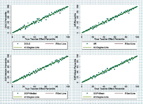
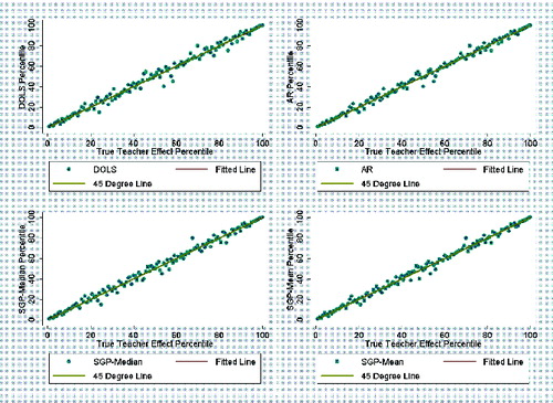
Figures 1 and 2 provide a visual illustration of the results for the random assignment cases. The figures display scatterplots of each teacher’s percentile in terms of their true teacher effect against the teacher’s percentile in terms of their teacher quality estimate. The points on the scatterplot are the average teacher quality estimate (either DOLS, AR, SGP-Median, or SGP-Mean) from across the 100 simulation repetitions, which is then converted to percentiles. Each teacher’s true teacher effect is held constant across the repetitions. The fitted lines are derived from a local polynomial smoother. A 1 degree polynomial is used in the smoothing. Figure 1 displays the RG-RA scenario and Figure 2 displays the DG-RA scenario. As both figures show, all estimators perform more or less equally well in capturing true teacher effects.

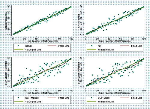
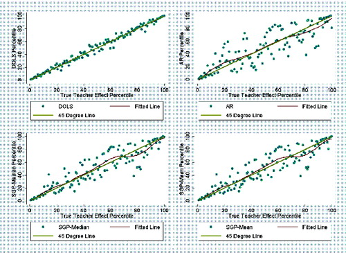
Figure 3 illustrates the marked decrease in the performance of the SGP estimators, as well as the decrease, somewhat less severe, in the performance of the AR estimator under dynamic grouping with positive assignment (DG-PA). The performance of DOLS, on the other hand, looks fairly similar to its performance in the random assignment scenario. Figure 4 illustrates similar differences for the DG-NA scenario.

Figure 1 Plots of true teacher effect percentiles on DOLS, AR, SGP-Median, and SGP-Mean percentiles using simulated data—RG-RA scenario.

3.3 Simulation Results for Sensitivity Analyses

Our simulations are intentionally simplified to highlight the behavior of the estimators we consider under conditions of random and nonrandom assignment. For example, for simplicity, we have thus far used a data-generating process in which the relationship between current and prior scores is linear. To relax this restriction and test the sensitivity of our results to this assumption, we also generated test score data in which a squared prior year test score term is included in the data-generating process. In this case, the SGP estimators can outperform DOLS when the generated coefficient on the squared term is set to an implausibly large number such as 1 (results are not reported but are available upon request). However, the difference is driven simply by the functional form in which prior test scores enter the model. Once the DOLS specification is rendered more flexible by including a polynomial or B-spline function of prior test scores, it regains its status as the best estimator across random and nonrandom assignment scenarios in the simulation.

Figure 2 Plots of true teacher effect percentiles on DOLS, AR, SGP-Median, and SGP-Mean percentiles using simulated data—DG-RA scenario.

Moreover, it is unlikely that nonlinear relationships between current and prior scores are a significant feature of real data. In our actual data, we find that the coefficient on the squared term in a regression of math achievement on math prior achievement, prior achievement squared, other student demographics, and teacher indicators is estimated to be around 0.05 rather than an unrealistically large number like 1. Moreover, when we compare estimated teacher effects from the basic DOLS estimator with those from a DOLS estimator that includes the square and cube of prior year test scores in the real data, we find that the estimates are very highly correlated (around 0.99), signaling that nonlinearities do not occur in real data in a way that impacts teacher quality measures.

Figure 3 Plots of true teacher effect percentiles on DOLS, AR, SGP-Median, and SGP-Mean percentiles using simulated data—DG-PA scenario.

Figure 4 Plots of true teacher effect percentiles on DOLS, AR, SGP-Median, and SGP-Mean percentiles using simulated data—DG-NA scenario.

Also in an effort to keep the simulation simple, we did not include other demographic characteristics of students, such as, say, English Language Learner (ELL) status, in the test-score data-generating process, nor did we sort students on the basis of these characteristics in our simulation. However, it would logically follow that a DOLS-type estimator that also controls for such observables will outperform the other estimators under nonrandom assignment based on these characteristics, since neither the SGP nor the AR models control for teacher assignment and the SGP estimators typically omit student demographics altogether.

One claim that could be made about the SGP approaches is that the teacher rankings may be more robust to outliers, since the quantile regression estimators used in the ranking method are themselves less affected by outliers. If the distribution is thicker tailed, the SGP model may perform better than the estimators based on OLS. As a further robustness check, therefore, we examine the performance of the estimators when the idiosyncratic error term u_i3 is drawn from a t-distribution with 3 degrees of freedom (df). The t-distribution with 3 df has much thicker tails than the normal distribution.

Results are reported in Table 2. Under random grouping and random assignment (RG-RA), the SGP-Median and particularly the SGP-Mean estimators outperform the value-added estimators. The SGP-Median estimator has a rank correlation of 0.72, and the SGP-Mean estimator has a rank correlation of 0.79 in the λ = 1 case. The value-added estimators have a slightly lower rank correlation of 0.71.

Table 2 Rank correlations and misclassification measures across estimators with simulated data generated with (3) errors. Results from 100 replications. Row 1: average rank correlation. Row 2: percentage of teachers above bottom 25% in true effect misclassified in bottom 25%. Row 3: percentage of teachers in bottom 25% in true effect misclassified in top 75%

					Corr DOLS/
Estimator	DOLS	AR	SGP-median	SGP-mean	SGP-median
Assign mech
	λ = 1
RG-RA	0.71	0.71	0.72	0.79	0.85
	13%	13%	13%	12%
	40%	40%	39%	35%
DG-RA	0.72	0.72	0.71	0.78	0.84
	12%	12%	13%	12%
	36%	36%	38%	36%
DG-PA	0.70	0.58	0.57	0.66	0.80
	13%	15%	16%	15%
	39%	46%	48%	44%
DG-NA	0.71	0.59	0.59	0.66	0.80
	13%	14%	15%	14%
	38%	47%	45%	43%
	λ = 0.5
RG-RA	0.71	0.71	0.71	0.79	0.85
	13%	13%	13%	12%
	40%	40%	39%	35%
DG-RA	0.72	0.72	0.71	0.78	0.84
	12%	12%	13%	12%
	36%	36%	38%	35%
DG-PA	0.70	0.58	0.57	0.66	0.80
	13%	15%	16%	15%
	39%	46%	48%	44%
DG-NA	0.71	0.59	0.59	0.66	0.80
	13%	16%	15%	14%
	38%	47%	45%	43%

Under the dynamic grouping and nonrandom assignment (DG-PA and DG-NA) scenarios, however, DOLS again outperforms the SGP estimators, which do not properly partial out the relationship between the covariates and the teacher’s value-added. The rank correlation for DOLS remains relatively stable at 0.70 and 0.71 for the DG-PA and DG-NA scenarios in the λ = 1 case. The rank correlation for the SGP-Median estimator drops to 0.57 and 0.59 for the DG-PA and DG-NA scenarios, and the rank correlation drops to 0.66 and 0.66 for the SGP-Mean estimator.

An important takeaway from this sensitivity analysis is that there may be cases in which using the SGP estimators is preferable. One such case may be when the distribution is thick tailed and there is random grouping and assignment. However, as the simulations show, even in the thick tailed case, nonrandom grouping and assignment still pose a threat to the SGP estimators.

4. EMPIRICAL ANALYSIS

We now examine the correlations between the estimators using real data. A main finding from the simulations was that the DOLS and SGP estimators provide similar rankings under random assignment but somewhat different rankings under nonrandom assignment. Using real data, we would therefore expect to find patterns suggesting a similar relationship between DOLS and SGP estimators when comparing correlations for teachers in schools with little evidence of nonrandom grouping with those for teachers in schools with evidence of nonrandom grouping.

Table 3 Spearman rank correlations across estimators for nonrandom grouping and random grouping schools in administrative dataset. Grades 5 and 6. Years 2002–2007

Variables	DOLS	EB-Lag	SGP-Median	SGP-Mean
Panel A: Random grouping schools
DOLS	1.000
EB-Lag	0.990	1.000
SGP-Median	0.912	0.901	1.000
SGP-Mean	0.929	0.914	0.981	1.000
Teacher/Year Obs	457	457	457	457
Panel B: Nonrandom grouping schools
DOLS	1.000
EB-Lag	0.985	1.000
SGP-Median	0.891	0.875	1.000
SGP-Mean	0.912	0.895	0.982	1.000
Teacher/Year Obs	1061	1061	1061	1061

4.1 Data

We use administrative data from a large and diverse anonymous school district in a southern state. The data consist of 215,411 student year observations from years 2002–2007 and grades 5 and 6. Student-teacher links are provided. Also, basic student information, such as demographic and socio-economic status, are available. The data include vertically scaled achievement scores in reading and math on a state criterion referenced test. Our analysis focuses on effectiveness estimates for mathematics teachers.

We imposed some exclusion restrictions on the data to accurately identify the parameters of interest. Students who cannot be linked to a teacher are dropped, as are students linked to more than one teacher in a school year in the same subject. Students in schools with fewer than 20 students are dropped, and students in classrooms with fewer than 12 students are dropped. Students who did not have two consecutive years of test scores are dropped. Students in charter schools are not included in this analysis, since charter schools may employ a set of teachers who are somewhat different from those typically found in public schools. Characteristics of the final dataset are reported in the appendix. These restrictions eliminated around 22.43% of observations in fifth grade and 20.24% of observations in sixth grade.

4.2 Analysis of Administrative Data

The simulation results indicated that in situations where students were both dynamically grouped based on prior year test scores and nonrandomly assigned to teachers, the DOLS estimator maintained a strong correlation with the true teacher effect, while the SGP estimator performed less well. To examine whether the SGP model differs from DOLS in actual data, we divided teachers into schools with random and nonrandom grouping using a test for nonrandomness developed in Dieterle et al. (2015). The test involves running a student-level multinomial logit regression of classroom assignment on prior year test scores and other observables for each school-grade-year combination in the data. Finding that students’ prior year test scores significantly predict their classroom assignment is taken as evidence that nonrandom grouping based on prior test scores occurs in that particular school-grade-year. Since nonrandom grouping is a precondition for nonrandom grouping and assignment, we focus on teachers in school years that reject the test of random grouping and compare them with teachers in school years that fail to reject. The data contain 305 unique schools with 1025 unique school-year-grade observations for which we could perform the multinomial logit test (more than one classroom per grade is needed to perform the test). Out of the 1025 school-year-grade observations, there is evidence of nonrandom grouping in 845 (60.88%). We report Spearman rank correlations across estimators as well as differences in classification: the fraction of teachers rated in the bottom (or top) 25% in one estimator but not in the other. These comparison measures are presented in Tables 3 through 5. Although our main focus is the comparison between the DOLS and SGP estimators, we also include statistics for the empirical Bayes' estimator, which we abbreviate as EB-Lag, in our comparison. The results for the AR estimator are available upon request. The correlation between the two estimators is 0.998, and the results for the shrunken AR estimator are very similar to those derived from the empirical Bayes' estimator.

The DOLS and EB-Lag models include the student’s free-and-reduced price lunch status, English learner status, gender, and indicators for whether the student is black or Hispanic. Teacher effectiveness estimates for all estimators—DOLS, EB-Lag, and SGP—are computed using data from two student cohorts. We use six years of chronological data, but each teacher estimate is a two year average. We also computed estimates based on one student cohort, but in this case the DOLS specification did not include peer characteristics. The resulting patterns were similar to those presented here and are available upon request. The DOLS and the EB-Lag models include two prior years mathematics scores as controls, as well as the student’s class average prior year test score as a control for peer effects. The SGP models include only the two prior year mathematics scores as controls in the quantile regressions, since this is how the estimator is described in Betebenner (2011). As a sensitivity check we estimate the SGP rankings by including the other student demographics. In another sensitivity check, we estimate the value-added models using only previous test scores as controls. This somewhat alters the correlations, but the main patterns still hold.

Table 4 Fraction of teachers rated in bottom 25% in the initial estimator who are not rated in bottom 25% in another estimator for nonrandom grouping and random grouping schools

Variables	DOLS	EB-Lag	SGP-Median	SGP-Mean
Panel A: Random grouping schools
DOLS	0	0.043	0.174	0.165
EB-Lag	0.043	0	0.157	0.157
SGP-Median	0.174	0.157	0	0.087
SGP-Mean	0.165	0.157	0.087	0
Teacher/Year Obs	457	457	457	457
Panel B: Nonrandom grouping schools
DOLS	0	0.09	0.222	0.18
EB-Lag	0.09	0	0.218	0.203
SGP-Median	0.222	0.218	0	0.09
SGP-Mean	0.18	0.203	0.09	0
Teacher/Year Obs	1061	1061	1061	1061

We separated teachers into the nonrandom grouping and random grouping categories based on the same two cohorts of data used for the teacher quality estimates. The nonrandom grouping category is defined as the set of teachers observations in schools in which the multinomial logit test rejected in both the student cohorts in which his or her teacher’s effectiveness estimate was calculated. The random grouping category is defined as the set of teachers observations in school-grades where the test failed to reject in both cohorts. There were 459 two-cohort school-grade observations that were classified as nonrandom grouping. There were 232 that were classified as random grouping. There were 334 that had mixed grouping over the two cohorts of students.

Table 5 Fraction of teachers rated in top 25% in the initial estimator who are not rated in top 25% in another estimator for nonrandom grouping and random grouping schools

Variables	DOLS	EB-Lag	SGP-Median	SGP-Mean
Panel A: Random grouping schools
DOLS	0	0.079	0.202	0.175
EB-Lag	0.079	0	0.193	0.184
SGP-Median	0.202	0.193	0	0.096
SGP-Mean	0.175	0.184	0.096	0
Teacher/Year Obs	457	457	457	457
Panel B: Nonrandom grouping schools
DOLS	0	0.079	0.211	0.189
EB-Lag	0.079	0	0.249	0.211
SGP-Median	0.211	0.249	0	0.083
SGP-Mean	0.189	0.211	0.083	0
Teacher/Year Obs	1061	1061	1061	1061

Based on the simulations, we expect that the rank correlations across estimators will be higher in schools where there is little or no evidence of nonrandom grouping, and we find evidence to suggest this. As shown in Table 3, the correlation between DOLS and SGP-Median is 0.912 in random grouping schools and 0.891 in nonrandom grouping schools. The corresponding correlations between DOLS and SGP-Mean are 0.929 and 0.912, respectively. The DOLS and EB-Lag estimators are more highly correlated due to the similarity in their specifications—however, these also exhibit a slight decrease in correlation in the nonrandom grouping context. All the reported differences are relatively slight, but it must be remembered that the simulation illustrated that nonrandom grouping became a threat to value-added estimation only when it was coupled with nonrandom assignment of classrooms to teachers. Unfortunately, in real data, we cannot effectively distinguish random and nonrandom assignment cases—we can only detect nonrandom grouping, which is a necessary but not sufficient condition for nonrandom grouping and assignment. Thus, our nonrandom grouping subsample contains a mixture of teachers who have been randomly and nonrandomly assigned to classrooms. It is not possible to know how much positive or negative assignment occurs, but it is certainly plausible that some principals assign ability-grouped classrooms purposefully to teachers based on their effectiveness while others may simply assign such classrooms randomly to teachers each year.

In Tables 4 and 5, we report the extent of disagreement between the estimators in terms of who is classified in the bottom and top 25% of teachers. Similar to the pattern indicated by the rank correlations, there is less disagreement between the estimators for teachers in schools with random grouping. For example, with regard to classification in the bottom 25% of the effectiveness distribution shown in Table 4, 17% of teachers are rated differently by DOLS and the SGP-Median estimator in the random grouping subsample but 22% of teachers are rated differently in the nonrandom grouping subsample. The classification differences at the top of the distribution, shown in Table 5, are slightly less pronounced but nonetheless in the expected direction.

5. CONCLUSIONS

In this article, we compare commonly used value-added estimators to two SGP models: one based on the median student growth percentile for students assigned to the teacher and the other based on the mean.

Simulation evidence indicates that the relative performance of these estimators depends on how students are grouped and assigned to teachers. In cases where students are nonrandomly grouped based on prior year test scores and nonrandomly assigned to teachers, the SGP estimators perform poorly compared with the DOLS estimator, which partials out the relationship between student’s prior year achievement and the teacher assignment.

A key result from the simulation is that DOLS, because it controls for teacher assignment in estimating the parameters on the other covariates, including lagged test scores, outperforms not only SGP estimators but also value-added models that do not control for teacher assignment when assignment is nonrandom.

The performance of the estimators also depends to some extent on the distribution of the error term in the achievement model. When a fatter tailed t-distribution with 3 df is used for the error term in our simulations, DOLS and the other value-added estimators perform worse than the SGP estimators in the random assignment scenario, but only slightly so. DOLS still outperforms the SGP estimators in the nonrandom grouping and assignment scenarios.

Additionally, we compare the estimators using actual data. In accordance with the predictions of the simulation analysis, we detect greater divergence between the DOLS and SGP estimates for teachers in school contexts that exhibit evidence of nonrandom grouping than for teachers in school contexts in which grouping is fairly random.

This article provides evidence that nonrandom grouping and assignment can negatively affect the popular SGP modeling approaches. Care should be taken by practitioners and researchers in evaluating teachers using these approaches when nonrandom grouping and assignment occurs in the school system. More generally, estimators that partial out teacher effects are better equipped to disentangle teacher contributions to student achievement from other factors affecting achievement than estimators that do not adjust for teacher assignment, whether they be SGPs or VAMs.

Additional information

Notes on contributors

Cassandra Guarino

Cassandra Guarino, Department of Educational Leadership and Policy Studies, School of Education, Indiana University, Bloomington, IN 47405 (E-mail: [email protected]). Mark Reckase, Department of Counseling, Educational Psychology, and Special Education, Michigan State University, East Lansing, MI 48824 (E-mail: [email protected]). Brian Stacy, Michigan State University, East Lansing, MI 48824 (E-mail: [email protected]). Jeffrey Wooldridge, Department of Economics, Michigan State University, East Lansing, MI 48824 (E-mail: [email protected]).

Mark Reckase

Cassandra Guarino, Department of Educational Leadership and Policy Studies, School of Education, Indiana University, Bloomington, IN 47405 (E-mail: [email protected]). Mark Reckase, Department of Counseling, Educational Psychology, and Special Education, Michigan State University, East Lansing, MI 48824 (E-mail: [email protected]). Brian Stacy, Michigan State University, East Lansing, MI 48824 (E-mail: [email protected]). Jeffrey Wooldridge, Department of Economics, Michigan State University, East Lansing, MI 48824 (E-mail: [email protected]).

Brian Stacy

Cassandra Guarino, Department of Educational Leadership and Policy Studies, School of Education, Indiana University, Bloomington, IN 47405 (E-mail: [email protected]). Mark Reckase, Department of Counseling, Educational Psychology, and Special Education, Michigan State University, East Lansing, MI 48824 (E-mail: [email protected]). Brian Stacy, Michigan State University, East Lansing, MI 48824 (E-mail: [email protected]). Jeffrey Wooldridge, Department of Economics, Michigan State University, East Lansing, MI 48824 (E-mail: [email protected]).

Jeffrey Wooldridge

Cassandra Guarino, Department of Educational Leadership and Policy Studies, School of Education, Indiana University, Bloomington, IN 47405 (E-mail: [email protected]). Mark Reckase, Department of Counseling, Educational Psychology, and Special Education, Michigan State University, East Lansing, MI 48824 (E-mail: [email protected]). Brian Stacy, Michigan State University, East Lansing, MI 48824 (E-mail: [email protected]). Jeffrey Wooldridge, Department of Economics, Michigan State University, East Lansing, MI 48824 (E-mail: [email protected]).

Notes

This distinction permits policymakers and others to claim that growth models are not value-added models.

Vertically scaled test scores allow for a comparison of student knowledge across years. In theory, with a vertical scale, a student score of 500 in third grade and a score of 550 in fourth grade would indicate that the student made a 50-point learning gain. However, it is sometimes the case that so-called vertical scales produce very similar scores for individual students from year to year, leading one to question whether they truly capture growth over time. The issue of whether the vertical scales can successfully be produced by test developers is controversial. For instance, Ballou (2009) and Barlevy and Neal (2011) critiqued the use of a vertical scale in teacher performance evaluation, and Briggs and Weeks (2009) showed that school-level value-added estimates can be sensitive to different scaling methods.

There are other percentile (or rank) based methods that are similar to the SGP methods, such as the approach proposed by Barlevy and Neal (2011) as a basis for distributing merit pay to teachers and applied by Fryer et al. (2012) in an experimental context, although its use in accountability policies is rare. The method consists of matching students based on their test score histories. Each student is matched to nine other students in, say, the district, with similar prior year test scores, and then teachers are evaluated on how their students compare to the nine other students they are matched with. We have examined the matching estimator proposed by Fryer et al. (2012) using our simulations and found that it performed similarly to the SGP methods evaluated.

These knots were chosen based on a phone conversation with Dr. Damian Betebenner.

These relative effect sizes are based on prior research [e.g., Nye, Konstantopoulos, and Hedges 2004; McCaffrey et al. 2004; Lockwood et al. 2007]. We changed the relative effect sizes in several sensitivity checks and found no substantive differences in resulting patterns. That said, however, the larger the relative size of teacher effects, the more accurately the models capture the true effects. See Guarino, Reckase, and Wooldridge [2015] for a more thorough discussion of these sensitivity checks.

A.1. Appendix of Tables

Appendix A Summary statistics for administrative data

Grade 5
Student-level characteristics
Variable	Mean	Std. Dev.	Min.	Max.
Math scale score	1630.033	239.368	569	2456
Reading scale score	1552.276	321.701	474	2713
Black	0.281	0.45	0	1
Hispanic	0.597	0.491	0	1
Free and reduced price lunch	0.703	0.457	0	1
Limited English proficiency	0.507	0.5	0	1
N	110,970
Teacher-level characteristics
Avg. lag Math score	1456.094	152.644	806.769	1986.808
Prop. FRL	0.718	0.249	0	1
Prop. LEP	0.508	0.259	0	1
Prop. Hispanic	0.584	0.322	0	1
Prop. Black	0.3	0.341	0	1
Number of students per year	24.019	7.929	12	145
Teacher experience	9.374	10.101	0	47
N	4620
Grade 6
Student-level characteristics
Math scale score	1641.693	247.982	770	2492
Reading scale score	1618.179	311.402	539	2758
Math scale standardized score	0.14	0.971	3.707	3.354
Reading scale standardized score	0.192	0.969	4.049	3.526
Black	0.288	0.453	0	1
Hispanic	0.6	0.49	0	1
Free and reduced price lunch	0.705	0.456	0	1
Limited English proficiency	0.511	0.5	0	1
N	104,441
Teacher-level characteristics
Avg. lag Math score	1608.182	143.225	903.733	2053.576
Prop. FRL	0.727	0.218	0	1
Prop. LEP	0.515	0.238	0	1
Prop. Hispanic	0.589	0.31	0	1
Prop. Black	0.307	0.33	0	1
Number of students per year	65.113	42.807	12	216
Teacher experience	7.668	8.978	0	40
N	1604

References

- Aaronson, D., Barrow, L., Sander, W. (2007), Teachers and Student Achievement in the Chicago Public High Schools, Journal of Labor Economics, 25, 95–135.
- Ballou, D. (2009), Test Scaling and Value-Added Measurement, Education Finance and Policy, 4, 351–383.
- Barlevy, G., Neal, D. (2011), Pay for Percentile, NBER Working Paper No. 17194, National Bureau of Economic Research.
- Betebenner, D.W. (2009), Norm-and Criterion-Referenced Student Growth, Educational Measurement: Issues and Practice, 28, 42–51.
- ——— (2011), A Technical Overview of the Student Growth Percentile Methodology: Student Growth Percentiles and Percentile Growth Projections/Trajectories, Technical Report, The National Center for the Improvement of Educational Assessment.
- ——— (2012), Growth, Standards, and Accountability, in Setting Performance Standards: Foundations, Methods & Innovations, ed. G. J. Cizek, New York: Routledge. pp. 439–450.
- Bibler, A.J., Guarino, C.M., Reckase, M.D., Vosters, K.N., Wooldridge, J.M. (2014), Precision for Policy: Calculating Standard Errors in Value-Added Models, unpublished manuscript.
- Briggs, D.C., Weeks, J.P. (2009), The Sensitivity of Value-Added Modeling to the Creation of a Vertical Score Scale, Education Finance and Policy, 4, 384–414.
- Dieterle, S.G., Guarino, C.M., Reckase, M.D., Wooldridge, J.M. (2015), How Do Principals Assign Students to Teachers? Finding Evidence in Administrative Data and the Implications for Value-Added, Journal of Policy Analysis and Management, 34, 32–58.
- Ehlert, M., Koedel, C., Parsons, E., Podgursky, M. (2014), Selecting Growth Measures for School and Teacher Evaluations: Should Proportionality Matter? doi: (in press). 10.1177/0895904814557593.
- ——— (2013b), The Sensitivity of Value-Added Estimates to Specification Adjustments: Evidence From School- and Teacher-Level Models in Missouri, Statistics and Public Policy, 1, 19–27.
- Fryer, R.G., Levitt, S.D., List, J., Sadoff, S. (2012), Enhancing the Efficacy Of Teacher Incentives Through Loss Aversion: A Field Experiment, NBER Working Paper No. 18237, National Bureau of Economic Research.
- Goldhaber, D., Walch, J., Gabele, B. (2013), Does the Model Matter? Exploring the Relationship Between Different Student Achievement-Based Teacher Assessments, Statistics and Public Policy, 1, 28–39.
- Guarino, C. M., Maxfield, M., Reckase, M. D., Thompson, P., and Wooldridge, J. M. ( 2015), An Evaluation of Empirical Bayes Estimation of Value-Added Teacher Performance Measures,” Journal of Educational and Behavioural Statistics, 40, 190–222.
- Guarino, C.M., Reckase, M.D., Wooldridge, J.M. (2015), Can Value-Added Measures of Teacher Performance be Trusted?, Education Finance and Policy, 10, 117–156.
- Hanushek, E.A. (1979), Conceptual and Empirical Issues in the Estimation of Educational Production Functions, Journal of Human Resources, 351–388.
- Harris, D., Sass, T., Semykina, A. (2014), Value-Added Models and the Measurement of Teacher Productivity,” Economics of Education Review, 38, 9–23.
- Lockwood, J., McCaffrey, D.F., Hamilton, L.S., Stecher, B., Le, V.-N., Martinez, J.F. (2007), The Sensitivity of Value-Added Teacher Effect Estimates to Different Mathematics Achievement Measures, Journal of Educational Measurement, 44, 47–67.
- McCaffrey, D.F., Lockwood, J., Koretz, D., Louis, T.A., Hamilton, L. (2004), Models for Value-Added Modeling of Teacher Effects, Journal of Educational and Behavioral Statistics, 29, 67–101.
- Nye, B., Konstantopoulos, S., Hedges, L.V. (2004), How Large are Teacher Effects? Educational Evaluation and Policy Analysis, 26, 237–257.
- Todd, P.E., Wolpin, K.I. (2003), On the Specification and Estimation of the Production Function for Cognitive Achievement, The Economic Journal, 113, F3–F33.
- Wright, S.P., White, J.T., Sanders, W.L., Rivers, J.C. (2010), Sas® Evaas® Statistical Models, SAS White Paper.