Using Graphical Models to Examine Value-Added Models

ABSTRACT

Value-added models (VAMs) of student test scores are used within education because they are supposed to measure school and teacher effectiveness well. Much research has compared VAM estimates for different models, with different measures (e.g., observation ratings), and in experimental designs. VAMs are considered here from the perspective of graphical models and situations are identified that are problematic for VAMs. If the previous test scores are influenced by variables that also influence the true effectiveness of the school/teacher and there are variables that influence both the previous and current test scores, then the estimates of effectiveness can be poor. Those using VAMs should consider the models that may give rise to their data and evaluate their methods for these models before using the results for high-stakes decisions.

KEYWORDS:

• Bayes nets
• Causality
• Directed acyclic graphs
• School effectiveness
• Teacher effectiveness

1. Introduction

Estimating causal effects is important within education. This includes, in many countries, using students’ test scores to estimate the relative causal effects of schools and teachers. A statistical model often used to make these estimates is called the value-added model (VAM) by education researchers in the U.S. This name is perhaps unfortunate because it presumes that the procedure accurately measures the causal impact of schools and teachers whenever the model is applied. The primary goal of this article is to identify if there are situations where this name may not be appropriate.

Using test scores to evaluate schools and teachers is one of the most important and hotly debated policy issues in education because the results from VAMs influence high-stakes decisions. There has been much research comparing VAM estimates from (often slightly) different statistical models, comparing VAM estimates with other measures like observational ratings, and comparing VAM estimates within studies that use random assignment (reviews include: Raudenbush and Willms 1995; Goldstein and Spiegelhalter 1996; Raudenbush 2004; Braun 2005; Baker et al. 2010; Wainer 2011; Foley and Goldstein 2012; McCaffrey 2012; Castellano and Ho 2013; Haertel 2013; Amrein-Beardsley 2014; Goldhaber et al. 2014; Goldstein 2014; Koedel et al. 2015).

The example used throughout this article will be for assessing schools because of the importance placed on measuring school effectiveness due in part to No Child Left Behind and subsequent legislation in the U.S. (e.g., Every Student Succeeds Act), and initiatives in other countries (e.g., House of Commons: Children, Schools and Families Committee 2007–2008; Manzi et al. 2014). This is often discussed with the labels “league tables” and “school effectiveness,” especially outside of the U.S. These methods are also used to assess relative causal effects in other areas including crime and health (Foley and Goldstein 2012).

There has been interest in assessing value-added within education for several decades (Hanushek 1971). Early examples of VAMs include Nuttall et al. (1989) for comparing schools and Sanders and Horn (1994) for comparing teachers. However, since their inception even some of those integral to the development of VAMs have cautioned policy makers not to place too much trust in the procedure: a VAM is “most certainly not a magic wand that will allow us automatically to make definitive pronouncements about differences between individual schools” (Goldstein 1991, p. 91).

The purpose of this article is to examine causal models that might give rise to educational test data and to ask if the causal effect of interest, the direct effect from school effectiveness to students’ test scores, can be accurately measured from a statistical model that is commonly used. As stated, this is a large research area, with many excellent reviews and therefore details will not be repeated. Most of the research has reported the associations between the estimated value-added scores using different models of the test data and using different types of data (e.g., student surveys). Much of the discussion is about whether these associations are large enough to support the measures being used in high-stakes decisions. Here, the focus is on whether the VAM estimates of school effectiveness are similar to the true school effectiveness, not to other estimates that may have similar biases to the VAM estimates to which they are compared. Simulation methods are used to allow access to true school effectiveness values for the model assumed and therefore allow assessment of the validity of the statistical model.

2. Statistical Models

Several different statistical models can be used for modeling school effectiveness, and different notations are used. These vary by discipline (e.g., in statistics, education, economics). The terminology used here follows Goldstein (2011), which described one of the main approaches, using multilevel (also called mixed and hierarchical) models, for predicting student outcomes. It allows a random effect for schools. Other approaches, like treating the school estimates as fixed effects, are popular among economists (Koedel et al. 2015). These approaches usually yield similar estimates (Deming 2014), providing the schools are of similar size. A related model is the student growth model (SGM; Betebenner 2007; Lockwood and Castellano 2015). It uses quantile regressions to compare students with similar prior scores. The effects studied here for multilevel models are relatively analogous to student growth models, but are not studied directly here.

An important development in the 1980s for VAMs was the increased use of multilevel modeling within education (e.g., Aitken et al. 1981; Aitkin and Longford 1986). This approach allows the variability among schools to be estimated in an efficient manner. The question here is whether estimates related to this variability are accurate enough estimates of the true value-added effects to be used in high-stakes decision making and for research purposes. To illustrate the use of a VAM with educational data and to introduce some terminology, suppose that pre and post are scores for students nested within schools, the first occurring prior to when the student arrives at the school and the second when the student leaves the school. The following linear model predicts post scores from pre scores: (1) $$\begin{array}{c}\hfill {\text{post}}_{ij}={\beta }_0+{\beta }_1{\text{pre}}_{ij}+u_j+e_{ij},\end{array}$$(1) where i indexes students and j indexes schools. The e_ij are the student residuals within the school. Further, additional predictors are commonly included on the right-hand side of (1). The term u_j is critical for these models. Estimates of u_j are used to estimate the conditional means (for linear models these are equivalent to the more general term conditional modes). These conditional means are used to estimate how much above or below the average school the jth school’s intercept appears to be conditional on the other variables included in the model (Goldstein 2011). The critical assumption for many decisions based on VAMs is interpreting these conditional means (often called school residuals) as measures of the causal variable often called school effectiveness. These are the estimated value-added scores.

It is standard practice to assume that both e_ij and u_j are normally distributed. There are other assumptions in the regression model shown in (1(1) $$\begin{array}{c}\hfill {\text{post}}_{ij}={\beta }_0+{\beta }_1{\text{pre}}_{ij}+u_j+e_{ij},\end{array}$$(1) ). Of particular relevance to this article, the statistical model assumes ${\text{pre}}_{ij}$ is independent of u_j. However, in the typical value-added situation, ${\text{pre}}_{ij}$ is associated with u_j (Spencer 2008). A goal of this article is to show when this may be problematic.

The VAM in (1(1) $$\begin{array}{c}\hfill {\text{post}}_{ij}={\beta }_0+{\beta }_1{\text{pre}}_{ij}+u_j+e_{ij},\end{array}$$(1) ) uses only the previous test scores as a predictor (or covariate). A VAM with two additional contextual variables, school economic status (SES) and IQ, is (2) $$\begin{array}{c}\hfill {\text{post}}_{ij}={\beta }_0+{\beta }_1{\text{pre}}_{ij}+{\beta }_2{\text{SES}}_j+{\beta }_3{\text{IQ}}_{ij}+u_j+e_{ij}.\end{array}$$(2) The choice of which variables to include will depend on the purpose for conducting the VAM (Raudenbush and Willms 1995). For example, if the goal were to evaluate schools then the analyst might want to condition on environmental factors and financial resources outside of the schools’ control. However, if the goal were to help parents to decide which schools would be best for their children, the analyst might not condition on these variables (though see Leckie 2009; Leckie and Goldstein 2009, for additional problems using VAMs for this purpose). The choice of whether to include these variables changes the meaning of u_j and therefore the meaning of the estimated value-added scores. In this article only the model in (1(1) $$\begin{array}{c}\hfill {\text{post}}_{ij}={\beta }_0+{\beta }_1{\text{pre}}_{ij}+u_j+e_{ij},\end{array}$$(1) ) is used, but the same arguments apply to the more complex statistical models.

It is worth noting that in special circumstances, other methods can be used. For example, situations in which students and teachers move between schools can be treated as a quasi-experiment. However, those students and teachers who move are not representative of all students and teachers. In other situations, there are lotteries for entering schools (e.g., Allen et al. 2013; Kane et al. 2013). Deming (2014) used a lottery situation to test the validity of different VAMs. Although he could not “reject the hypothesis the school effects are unbiased” (p. 406), meaning that the conditional means may be good estimates in this situation, he urged caution because the sample was small and limited to a single district (p. 409). Deming’s results are encouraging, but because lotteries are not common and tend to occur in atypical situations they cannot be used in general to estimate value-added scores (Allen et al. 2013, see also footnote 4).

3. Graphical Models

Although the popularity of graphical methods is increasing in educational assessment (e.g., Almond et al. 2015), the terminology of graphical models is still uncommon in most of the education literature, so deserves some introduction. A graph is a set of nodes connected by edges. These edges can be either directed or undirected. The direction is denoted by having an arrowhead on one end. A path is a series of nodes connected by edges with the restriction that none of the intermediate nodes are included more than once.

Drawing graphs can help to determine if effects can be accurately measured (for reviews, see Pearl 2009; Højsgaard et al. 2012; Elwart 2013; Pearl et al. 2016).¹ Figure 1 shows a causal model that includes the pre and post test scores, the true school value-added $\mathit{VA}$, and two un-measured variables called um1 and um2. The squares denote observed variables; the circles denote un-measured variables. Each node can be a variable or set of variables. For example, pre could represent several previous test scores, which would increase the reliability of the estimates for this node. Here the edges represent causal influences from one node to another in the direction of the arrow.²

Figure 1. A causal graph made with the plotmat function of the R package diagram (Karline Soetaert 2014).

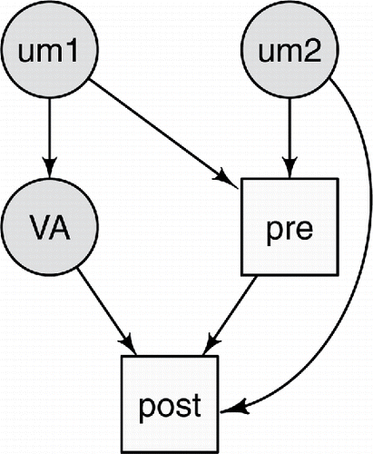
Figure 1 shows a simple model for how the pre and the post test scores might arise. The true value-added, $\mathit{VA}$, is not measured. The purpose of VAMs is to provide good estimates of these values. The primary purpose is not, for example, to try to predict post as accurately as possible. Let um1 be un-measured school-level variables that influence how the school performs. These may include school socio-economic status and neighborhood characteristics. It is assumed that they influence the school value-added and also previous test scores. Let um2 represents un-measured student-level variables, which may include a student’s effort and intelligence, as well as the home environment. It is assumed um2 influences both pre and post scores.

While there will likely be school and student level variables that are measured (i.e., additional squares could be added to the graph), there will always be influences that are not measured. As is true with all models, this is a simplification. For example, um1 and um2 may be related and this could be shown by another variable influencing both of these. More arrows could also be included. The question is whether the statistical model can accurately measure value-added with data created according to this relatively simple data model.

4. Causal Inference and Backdoor Paths

While graphical models can be used for several purposes, when applied to scientific data it is common practice to think of the nodes as variables and to think of directed edges as showing one variable influencing the other. For example, the path associated with the direct value-added effect is VA → post and this implies that what the school does affects post scores. This direct effect cannot be measured in isolation with most education data. The association between VA and post will be influenced by the direct causal path VA → post, but it can be affected by other so-called backdoor paths between VA and post (Pearl 2009, chap. 3). In Figure 1, there are two backdoor paths between VA and post:

(a)	VA ← um1 → pre → post and
(b)	VA ← um1 → pre ← um2 → post.

Much of the VAM literature pertains to path (a), but there is less discussion about path (b). The remainder of this section contrasts these two paths and how conditioning on pre affects them differently.

A path between two variables can either be unblocked or be blocked. If a path is unblocked it means that information can flow through the path. A useful metaphor is of water flowing within a river. If a dam is placed in the river, the path for the water is blocked. If a backdoor path between two variables is unblocked then this can confound the measurement of the direct effect between the variables because information can flow through the backdoor path. If two variables have both a direct path and an unblocked backdoor path, then the correlation between them will be influenced by both of these paths (Simon 1954).

To decide whether a path is blocked or unblocked, it is necessary to distinguish the three types of paths that can connect three variables: X, Y, and Z (which may be single variables or sets of variables). The three types of path are: chains (X → Y → Z), forks (X ← Y → Z), and colliders (X → Y ← Z). Pearl (2009, pp. 16–17) described two rules to test if a path from X to Z is blocked by conditioning on Y.

Rule #1. “The path must contain a chain or fork in which the middle variable is Y.”

Chains and forks are often discussed in the social science literature in relation to the phrases mediation and spurious correlation, respectively. An example of an unblocked chain is that turning on an oven causes the oven to heat up, and this causes food to cook. However, if you stop the oven from getting hot (e.g., leaving the oven door open), then turning on the oven will not cook the food. The causal path between turning the oven on and cooking the food is blocked by controlling the mediator, the heat of the oven. An example of a fork is the positive correlation between ice cream consumption and murder (Harper 2013). This is a spurious correlation because warm weather causes both of these to increase. If you condition on the weather, the path becomes blocked, and the spurious correlation disappears.

Rule #2. “The path contains a collider in which the middle variable (or any variable influenced by it) is NOT Y.”

There is less discussion about colliders within the social sciences. Using the river metaphor, imagine two tributaries arriving from different directions at a deep well. The deep well is the collider. The water from each would not reach the other; the path is blocked. If the well is filled with cement, water would flow between the tributaries and the path would be unblocked. Pearl et al. (2016) gave the example of a university that gives only two types of scholarships: for exceptional musical talent and for exceptional scholastic achievement. The path between musical talent and scholastic achievement has the collider, getting a scholarship, in the middle. The path from musical talent to scholastic achievement begins blocked. Suppose that in university population these two skills are unrelated. Learning that a student does not have exceptional musical talent provides no information about whether the student has exceptional scholastic achievement or not. However, once finding out the student has a scholarship, so conditioning on the collider (receiving a scholarship), it is immediately known that the scholarship student without musical talent must have exceptional scholastic achievement.

If either Rule #1 or Rule #2 is satisfied, then the path is blocked. In the graphing literature this is called d-separation. The first backdoor path, VA ← um1 → pre → post, can be blocked by conditioning on pre because pre is in the middle of a chain (Rule #1). If um1 had been measured, then it also could be used to block this path because it is in the middle of a fork (Rule #1). Most people using VAMs will be aware that conditioning on pre blocks this path. This is often given as one of the reasons for conditioning on pre as opposed to not conditioning on it (what are sometimes called status models).

The second backdoor path has a collider (pre). If a collider and all variables influenced by it (its descendants in causal modeling terminology) are not conditioned on then the path is blocked (Rule #2); information cannot flow along this path from $\mathit{VA}$ to post. But if pre is (or any of its descendants are) conditioned on, then the path becomes unblocked because pre is a collider. This situation is addressed here. According to Pearl’s rules, conditioning on pre can create problems for measuring school value-added scores because it unblocks the backdoor path VA ← um1 → pre ← um2 → post. The estimated value-added scores (i.e., the conditional means) are based on both the direct path VA → post and the unblocked backdoor path VA ← um1 → pre ← um2 → post.

5. Simulation

This section describes the simulation conducted to evaluate which situations are particularly problematic when the backdoor path VA ← um1 → pre ← um2 → post becomes unblocked by conditioning on pre. Using simulation methods is important because the true value of the school effectiveness can be known. With the analysis of real-world data, it is not possible to know the true value-added.

Figure 1 can be represented by the following equations if it is assumed that all the relationships are linear (linearity is not a requirement for Pearl’s rules, but is used here for purposes of illustration and is often assumed for VAMs) and each variable includes its own independent error term: (3) $$\begin{array}{c}\hfill \begin{array}{ccc}{\mathit{\text{VA}}}_j\hfill & =\hfill & {\beta }_1\text{um}{1}_j+e_j,\hfill \\ {\text{pre}}_{ij}\hfill & =\hfill & {\beta }_2\text{um}{1}_j+{\beta }_3\text{um}{2}_{ij}+e_{ij},\hfill \\ {\text{post}}_{ij}\hfill & =\hfill & {\beta }_4\text{um}{2}_{ij}+{\beta }_5{\mathit{\text{VA}}}_j+{\beta }_6{\text{pre}}_{ij}+e_{ij}.\hfill \end{array}\end{array}$$(3) There are no intercepts in these equations. For the simulation reported below, the error terms are all normally distributed with means of zero and standard deviations of one. The exogenous variables, um1 and um2, are also normally distributed.

The direct effect from VA → post is linear and in the simulations β₅ > 0. The correlations between the true value-added scores, VA_j, and the estimated value-added scores, $\widehat{{\mathrm{VA}}_j}$ (the conditional means), measure how accurate this procedure is. Policy makers must decide how high the correlation between these should be to justify using VAMs to allocate resources to schools or to affect teacher employment and morale. For linear models, the correlation is based on the sum of the products of all unblocked path coefficients. Sewall Wright (1934, p. 163) described this:

Any correlation between variables in a network of sequential relations can be analyzed into contributions from all of the paths (direct or through common factors) by which the two variables are connected, such that the value of each contribution is the product of the coefficients pertaining to the elementary paths.

It is predicted therefore that the product of the unblocked path coefficients will be negatively related to the correlation between the true and estimate value-added scores.

Most of the β values in (3(3) $$\begin{array}{c}\hfill \begin{array}{ccc}{\mathit{\text{VA}}}_j\hfill & =\hfill & {\beta }_1\text{um}{1}_j+e_j,\hfill \\ {\text{pre}}_{ij}\hfill & =\hfill & {\beta }_2\text{um}{1}_j+{\beta }_3\text{um}{2}_{ij}+e_{ij},\hfill \\ {\text{post}}_{ij}\hfill & =\hfill & {\beta }_4\text{um}{2}_{ij}+{\beta }_5{\mathit{\text{VA}}}_j+{\beta }_6{\text{pre}}_{ij}+e_{ij}.\hfill \end{array}\end{array}$$(3) ) describe relationships between unmeasured variables. It was decided in the simulation to have these cover a broad range of values for two reasons. First, it is unclear what all the un-measured variables that could be subsumed as part of um1, um2, and VA are. Second, even if the variables were known, estimating the relationships among un-measured variables is difficult. According to Bartholomew et al. (2011), “when we come to models for relationships between latent variables we have reached a point where so much has to be assumed that one might justly conclude that the limits of scientific usefulness have been reached, if not exceeded” (p. 228). Because of the wide range of β’s used, it is likely that realistic values will lie within this range (the range can be extended and this does not affect the conclusions). The results of the simulation reported below show that the association between true value-added scores and the conditional means varies with these β values. The critical assumption by those using VAMs for high-stakes decisions is that the conditional means accurately measure the true value-added scores.

Table 1 shows the values used for the simulation. The coefficients for the effects from the um variables were randomly drawn from a V-shaped distribution that was a distribution that ranged from (−2,2) to (0,0) to (0,2), but did not include points from −0.01 to +0.01. This distribution was used so that the products of the four coefficients were more spread out than if a uniform distribution were used. The values for the effects from VA and pre to post were chosen so that each of the eight combinations of these two factors occurred one-eighth of the time.

Table 1. The β values used to create data for the simulation.

Coefficient	Meaning	Values	How values are chosen
β1	um1 → VA	[−2,2]	V-shaped distribution
β2	um1 → pre	[−2,2]	V-shaped distribution
β3	um2 → pre	[−2,2]	V-shaped distribution
β4	um2 → post	[−2,2]	V-shaped distribution
β5	VA → post	0.1, 0.5, 1, or 2	Equal numbers of each
β6	pre → post	0.2 or 1	Equal numbers of each

This simulation was conducted using the R (v. 3.2.2) statistics environment (R Core Team 2016). The package lme4 (Bates et al. 2015) was used for multilevel estimation and the package triangle (Carnell 2016) was used for creating the V-shaped distribution. There were 20,000 replications. The code is in the supplementary materials. This allows others to replicate the findings and easily adapt the code to address other research questions. Further simulations and analyses, which reach the same main conclusion, are available from the author.

6. Results

Correlations between the true value-added scores and the estimated value-added scores ranged from near −0.9 to near +1.0 across the 20,000 simulated datasets. Seventy-two percent of the correlations were larger than 0.75 and 15% were less than or equal to zero. From Pearl’s rules, it is predicted that the backdoor path VA ← um1 → pre ← um2 → post will be problematic because conditioning on pre unblocks this path: Rule #2 from Pearl (2009, pp. 16–17). This path includes four edges, each with a corresponding β value that was allowed to range from −2 to 2. The correlation between two variables is the sum of the influence of each blocked path. The influence of each unblocked path is the product of the coefficients (e.g., Wright 1934; Loehlin 1998). The influence of the backdoor path, as measured by the product of the coefficients, that becomes unblocked by conditioning on pre, is predicted to be associated with the correlation between the true and estimated value-added scores.

Figure 2 summarizes the findings. The correlations between true and estimated value-added scores are plotted with the product of the backdoor path β values. The curves are 10 degree of freedom cubic splines. These splines were chosen in order that the curves would show the main trends in the data without much over-fitting. They show that the size of the correlation depends on the product of the coefficients of the critical backdoor path. The correlations are all fairly high when the product is negative. The mean correlation is 0.92 when this product was negative. The correlations are lower when the product is positive (the mean is 0.41) and the correlations decrease as the products increase. The dashed lines correspond to having only a small effect from pre to post (β₆ = 0.2) and the solid lines correspond to a large effect (β₆ = 1). The size of this effect makes little difference. This was expected as this edge is only part of a blocked backdoor path. If pre is not included in the model, the magnitude of this effect would matter because the path VA ← um1 → pre → post would be unblocked. The colors show the size of the true value-added effect VA → post. The black curve is the largest effect, the green curve is the next largest effect, and then blue and red. As the size of the true value-added effect increases, the correlations also increase. The means of the correlations when the product of the coefficients is negative are r = 0.82, r = 0.93, r = 0.97, and r = 0.99, for the true value-added (i.e., true school effectiveness) coefficients β₅ being 0.1, 0.5, 1, and 2, respectively. The corresponding means when the product is positive are: r = −0.51, r = 0.41, r = 0.84, and r = 0.97.

Figure 2. Results of the simulation. When the product of the unblocked path coefficients is greater than zero and the true VA effect is small, the estimates tend to be poor.

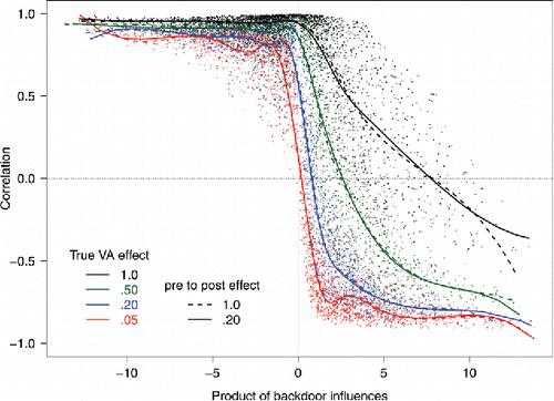
Hypothesis testing statistics support these conclusions. The first statistical model estimated used just the product of these four β’s to predict the correlation. Since the relationship is not assumed to be linear, a cubic regression spline with 10 degrees of freedom was used to draw a flexible curve through the data (other curves can also be used). This model accounted for adjusted R² = 0.27, F(10, 19989) = 750, p < 0.001. There are four levels for the path coefficient for VA → post (0.1, 0.5, 1, 2). If each is allowed its own curve the adjusted R² goes to 0.90, a significant increase in the fit of the model: F(33, 19956) = 3654, p < 0.001. The correlations are larger when the direct effect is larger. There are two levels for the pre → post effect. If each of the eight pre → post by VA → post combinations is allowed its own curve, the adjusted R² remains approximately the same, at 0.90, F(44, 19912) = 0.88.

7. Summary

Many policy makers treat the conditional means from value-added models (VAMs) as estimates of the causal effects of schools and teachers.³ This assumption may turn out to be correct, but historical precedent suggests caution. There are parallels with the movement among many social scientists at the end of the last century accepting, without appropriate caution, coefficients from regressions and structural equation models used on nonexperimental data as if they accurately estimated causal effects. Morgan and Winship (2007, p. 13) stated that this “naive usage of regression modeling was blamed for nearly all the ills of sociology.” Morgan and Winship stressed the fault was not in the regression equations. Their book describes how with care, appropriate data, and some assumptions causal estimates can be made. Their grievance was with the over-optimistic interpretation of these models’ estimates without describing the causal mechanisms. The movement to accept conditional means as estimates of causal effects may be similar.

VAMs are popular among some education policy makers who were promised that VAMs: “identify highly effective teachers and principals” (http://www.sas.com/en_us/industry/k-12-education/evaas.html, September 1, 2014). Further, studies like Deming’s (2014) suggest that VAMs produce estimates similar to those found in lottery studies.⁴ However, many statisticians are skeptical about their value. For example, Goldstein has stressed that VAMs have “some severe limitations that ought to make us think very carefully before using [them]” (1991). Further, Pearl’s (2009) guidelines for measuring causal effects show situations where the measurement of the direct causal effect is hampered by an unblocked backdoor path created by conditioning on previous test scores. A simulation was done to show that there is a relationship between the unblocked backdoor path coefficients and the extent of this problem.

The simulation shows when value-added estimates may be adequate measures of the true value-added and when they are likely to be poor. The estimates are likely to be poor if three conditions are met.

1.	There is an unblocked backdoor path (or multiple unblocked backdoor paths) between actual value-added and the final test scores.
2.	The product of the coefficients of this unblocked backdoor path is positive (and the larger the product is, the less accurate the estimates will likely be).
3.	The actual value-added effect is small compared with the product of the coefficients of the unblocked backdoor path (or the sum of the products of backdoor paths if there are several unblocked backdoor paths).

Regarding condition #1, within the social and educational sciences there will likely always be backdoor paths connecting the cause and the effect with nonexperimental designs. In terms of Figure 1, several additional nodes (which could be sets of measured and un-measured variables) could have been included creating several new backdoor paths. Only um1 and um2 were included here to simplify the data model for illustrative ease. It can be assumed that there will be some unmeasured variables that affect school effectiveness and previous test scores. It can also be assumed that there will be unmeasured variables that affect both pre and post test scores. Thus, it can be assumed that this backdoor path will exist. The current simulation had um1 vary only among schools (which could be neighborhood effects) and um2 vary within schools, but having variables at different levels does not affect the application of Pearl’s rules.

It is worth stressing that in Figure 1 there are only two backdoor paths between VA and post. A more developed model of student test scores will likely be more complex and have more backdoor paths. Careful consideration of how conditioning on covariates blocks or unblocks each of these paths should be considered. This is a difficult task. The American Statistical Association’s statement on VAMs includes: “VAMs are complicated statistical models, and they require high level of statistical expertise. Sound statistical practices need to be used when developing and interpreting them, especially when they are part of a high-stakes accountability system” (American Statistical Association 2014, p. 4). The relationships between variables are affected by unblocked paths. Correlations between conditional means and, for example, demographic variables that could be related to um1 and um2 should be viewed cautiously.

Regarding condition #2, the product of the path coefficients for the backdoor path considered in this article will be positive if the signs of the effects of um1 are the same on school effectiveness and pre scores, and if the signs of the effects of um2 are the same on the pre and on the post scores. Suppose um1 is some unmeasured characteristic that positively affects school quality, like aspects of the neighborhood. It should also positively influence previous schooling and pre scores. Therefore, β₁ and β₂ are likely to have the same sign. Similarly, if um2 is an unmeasured variable related to intelligence or effort, it should affect the pre and the post scores in similar ways. This means that β₃ and β₄ are likely to have the same sign. If β₁ and β₂ have the same sign and β₃ and β₄ have the same sign, then the product of the four of these will be positive.

Regarding condition #3, it is difficult to estimate the size of the true value-added effect, particularly in comparison with the magnitude of the backdoor paths. This is in part because of the difficulty of estimating relationships among un-measured variables (see the Bartholomew et al. 2011, quotation above). While the effects of years of a particular schooling program may be substantial, the simulation reported here should make readers cautious interpreting the results from VAMs if the true value-added effects are unlikely to be large. More research is necessary, but the current exploration of estimating causality using VAMs raises questions. Estimates of the effects for teachers should also be viewed cautiously if based on procedures like those examined here.

In conclusion, many policy makers want accurate measures of school and teacher effectiveness. The results presented here show that the conditional school means are based on both the true school effectiveness, which is the direct VA → post effect, and the unblocked backdoor path VA ← um1 → pre ← um2 → post. What should be done? First, if instrumental variables (here variables that influence only VA) are measured, these can be useful. Imbens and Rubin (2015) and Morgan and Winship (2007) provide good introductions to this approach. Second, because it is difficult to estimate how large the coefficients between un-measured variables are, it is necessary that if policy makers use a VAM that they argue why the potentially biasing effects of any unblocked backdoor paths will be small enough to be ignored. Finally, examining graphical models and using simulations are valuable techniques for assessing the worth of different statistical methods. The code in the supplementary materials can be adapted to explore other causal models. Future research using graphs may lead to better techniques for measuring school effectiveness.

Acknowledgments

The author thanks Judea Pearl, Lynn Mellor, and George Leckie for useful comments. Previously presented at the Texas Universities’ Educational Statistics and Psychometrics (TUESAP) meeting, 2015, University of Texas, Austin, TX, and the Inquiring Minds talk series, 2016, the Public Education Department, Santa Fe, NM.

Supplemental Materials

Code used for the simulation. Supplemental data for this article can be accessed on the publisher's website.

Notes

1 Not everyone finds drawing graphs helpful. Imbens and Rubin (2015) stated: “Pearl’s work is interesting, and many researchers find his arguments that path diagrams are a natural and convenient way to express assumptions about causal structures appealing. In our own work…we have not found this approach to aid drawing of causal inferences” (p. 22).

2 The pre scores themselves will not have a large (if any) influence on the post score. These scores are measures of knowledge at these points in time and it is this knowledge that will influence future knowledge. This graph could be expanded and have these nodes stand for knowledge at these points in time and have arrows from them pointed toward the measurements. The same general findings hold when the simulation is conducted in this way. The curves in Figure 2 (reported later in this article) shift toward r = 0 as the reliability of the scores decreases.

3 The argument to treat these as estimates of associations rather than of causes, but then have policy makers act as if they are causal, is not a good solution.

4 Figure 1 predicts that if random allocation is used then the VAM should be accurate because there will be no backdoor paths from $\mathit{VA}$. Finding that a model provides good estimates when there are no backdoor paths does not show that the model will work well when there are backdoor paths. The influence of backdoor paths is one of the main factors that questions the validity of these models.

References

- Aitken, M., Anderson, D. A., and Hinde, J. P. (1981), “Statistical Modelling of Data on Teaching Styles” (with discussion), Journal of the Royal Statistical Society, Series A, 144, 419–461.
- Aitkin, M., and Longford, N. (1986), “Statistical Modelling Issues in School Effectiveness Studies,” Journal of the Royal Statistical Society, Series A, 149, 1–43.
- Allen, R., Burgess, S., and McKenna, L. (2013), “The Short-Run Impact of Using Lotteries for School Admissions: Early Results From Brighton and Hove’s Reforms,” Transactions of the Institute of British Geographers, 38, 149–166.
- Almond, R. G., Mislevy, R. J., Steinberg, L. S., and Williamson, D. M. (2015), Bayesian Networks in Educational Assessment, New York: Springer.
- American Statistical Association (2014), “ASA Statement on Using Value-Added Models for Educational Assessment,” Technical Report, American Statistical Association. Accessed April 8, 2014, at http://www.amstat.or/asa/files/pdfs/POL-ASAVAM-Statement.pdf
- Amrein-Beardsley, A. (2014), Rethinking Value-Added Models in Education: Critical Perspectives on Tests and Assessment-Based Accountability, New York: Routledge.
- Baker, E. L., Barton, P. E., Darling-Hammond, L., Haertel, E., Ladd, H. F., Linn, R. L., Ravitch, D., Rothstein, R., Shavelson, R. J., and Shepard, L. A. (2010), “Problems with the Use of Student Test Scores to Evaluate Teachers,” Technical Report. Economic Policy Institute. Paper #278.
- Bartholomew, D. J., Knott, M., and Moustaki, I. (2011), Latent Variable Models and Factor Analysis: A Unified Approach (3rd ed.), Chichester, UK: Wiley.
- Bates, D., Mächler, M., Bolker, B., and Walker, S. (2015), “Fitting Linear Mixed-Effects Models Using, lme4” Journal of Statistical Software, 67, 1–48.
- Betebenner, D. W. (2007), Estimation of Student Growth Percentiles for the Colorado Student Assessment Program, National Center for the Improvement of Educational Assessment. Available at https://www.researchgate.net/publication/228822935
- Braun, H. I. (2005), “Using Student Progress to Evaluate Teachers:A Primer on Value-Added Models.” Educational Testing Service, NJ. Available at https://www.ets.org/research/policy_research_reports/publications/report/2005.cxje
- Carnell, R. (2016), triangle: Provides the Standard Distribution Functions for the Triangle Distribution, R Package Version 0.10. Available at https://CRAN.R-project.org/package=triangle.
- Castellano, K. E., and Ho, A. D. (2013), “A Practitioner’s Guide to Growth Models,” Available at http://scholar.harvard.edu/andrewho/publications/practitioners-guide-growth-models.
- Deming, D. J. (2014), “Using School Choice Lotteries to Test Measures of School Effectiveness,” American Economic Review: Papers & Proceedings, 104, 406–411.
- Elwart, F. (2013), “Causal Graphical Models,” in Handbook of Causal Analysis for Social Research, ed. Stephen L. Morgan, New York: Sage Publications, pp. 245–273.
- Foley, B., and Goldstein, H. (2012), Measuring Success: League Tables in the Public Sector, London: British Academy.
- Goldhaber, D., Walch, J., and Gabele, B. (2014), “Does the Model Matter? Exploring the Relationship Between Different Student Achievement-Based Teacher Assessments,” Statistics and Public Policy, 1, 28–39.
- Goldstein, H. (1991), “Better Ways to Compare Schools?” Journal of Educational Statistics, 16, 89–91.
- Goldstein, H. (2011), Multilevel Statistical Models (4th ed.), Chichester, UK: Wiley.
- Goldstein, H. (2014), “Using League Table Rankings in Public Policy Formation: Statistical Issues,” Annual Review of Statistics and its Application, 1, 385–399.
- Goldstein, H., and Spiegelhalter, D. J. (1996), “League Tables and Their Limitations: Statistical Issues in Comparisons of Institutional Performance” (with discussion), Journal of the Royal Statistical Society, Series A, 159, 385–443.
- Haertel, E. H. (2013), “Reliability and Validity of Inferences About Teachers Based on Student Test Scores. The 14th William H. Angoff Memorial Lecture,” Technical Report. Educational Testing Service, NJ. Available at http://www.ets.org/Media/Research/pdf/PICANG14.pdf.
- Hanushek, E. A. (1971), “Teacher Characteristics and Gains in Student Achievement: Estimation Using Micro-Data,” American Economic Review, 61, 280–288.
- Harper, J. (2013), “Ice Cream and Crime: Where Cold Cuisine and Hot Disputes Intersect,” available at http://www.nola.com/crime/index.ssf/2013/07/ice_cream_and_crime_where_hot.html.
- Højsgaard, S., Edwards, D., and Lauritzen, S. (2012), Graphical Models With R, New York: Springer-Verlag.
- House of Commons: Children, Schools and Families Committee., (2007), Testing and Assessment: Third Report of Session (Vol. 2), House of Commons: Children Schools and Families Committee, London, UK.
- Imbens, G. W., and Rubin, D. B. (2015), Causal Inference for Statistics, Social, and Biomedical Sciences: An Introduction, New York: Cambridge University Press.
- Kane, T. J., McCaffrey, D. F., Miller, T., and Staiger, D. O. (2013), “Have We Identified Effective Teachers? Validating Measures of Effective Teaching Using RandomAssignment.” Bill & Melinda Gates Foundation, Seattle, WA. Available at http://k12education.gatesfoundation.org/wp-content/uploads/2015/12/MET_Validating_Using_Random_Assignment_Research_Paper.pdf
- Karline Soetaert (2014), diagram: Functions for visualising simple graphs (networks), plotting flow diagrams. R package version 1.6.3. https://CRAN.R-project.org/package=diagram
- Koedel, C., Mihaly, K., and Rockoff, J. E. (2015), “Value-Added Modeling: A Review,” Economics of Education Review, 2, 1–9. DOI:10.1080/2330443X.2014.962718.
- Leckie, G. (2009), “The Complexity of School and Neighbourhood Effects and Movements of Pupils on School Differences in Models of Educational Achievement,” Journal of the Royal Statistical Society, Series A, 172, 537–554.
- Leckie, G., and Goldstein, H. (2009), “The Limitations of Using School League Tables to Inform School Choice,” Journal of the Royal Statistical Society, Series A, 172, 835–851.
- Lockwood, J. R., and Castellano, K. E. (2015), “Alternative Statistical Frameworks for Student Growth Percentile Estimation,” Statistics and Public Policy, 2.
- Loehlin, J. C. (1998), Latent Variable Models: An Introduction to Factor, Path, and Structural Analysis (3rd ed.), Mahwah, NJ: Erlbaum.
- Manzi, J., Martin, E. S., and Bellegem, S. V. (2014), “School System Evaluation by Value Added Analysis Under Endogeneity,” Psychometrika, 79, 130–153.
- McCaffrey, D. F. (2012), “Do Value-Added Methods Level the Playing Field for Teachers?,” available at carnegieknowledgenetwork.org/briefs/value-added/level-playing-field.
- Morgan, S. L., and Winship, C. (2007), Counterfactuals and Causal Inference: Methods and Principles for Social Research, Cambridge: Cambridge University Press.
- Nuttall, D. L., Goldstein, H., Prosser, R., and Rasbash, J. (1989), “Differential School Effectiveness,” International Journal of Education Research, 13, 769–776.
- Pearl, J. (2009), Causality: Models, Reasoning, and Inference (2nd ed.), New York: Cambridge University Press.
- Pearl, J., Glymour, M., and Jewell, N. P. (2016), Causal Inference in Statistics: A Primer, Chichester, UK: Wiley.
- Raudenbush, S. W. (2004), “What are Value-Added Models Estimating and What Does This Imply for Statistical Practice?” Journal of Educational and Behavioral Statistics, 20, 121–129.
- Raudenbush, S. W., and Willms, J. D. (1995), “The Estimation of School Effects,” Journal of Educational and Behavioral Statistics, 20, 307–335.
- R Core Team (2016), R: A Language and Environment for Statistical Computing, Vienna, Austria: R Foundation for Statistical Computing. Available at https://www.R-project.org/.
- Sanders, W. L., and Horn, S. P. (1994), “The Tennessee Value-Added Assessment System (TVAAS): Mixed Model Methodology in Educational Assessment,” Journal of Personnel Evaluation in Education, 8, 299–311.
- Simon, H. A. (1954), “Spurious Correlation: A Causal Interpretation,” Journal of the American Statistical Association, 49, 467–479.
- Spencer, N. H. (2008), “Models for Value-Added Investigations of Teaching Styles Data,” Journal of Data Science, 6, 33–51.
- Wainer, H. (2011), Uneducated Guesses: Using Evidence to Uncover Misguided Education Policies, Princeton, NJ: Princeton University Press.
- Wright, S. (1934), “The Method of Path Coefficients,” Annals of Mathematical Statistics, 5, 161–215.