Study of Salary Differentials by Gender and Discipline

ABSTRACT

Although it is 45 years since legislation made gender discrimination on university campuses illegal, salary inequities continue to exist today. The seminal work in studying the existence of salary inequities is that of the American Association of University Professors (AAUP), by Scott (1977) and Gray (1980). Subsequently, innumerable analyses based on versions of their multiple regression model have been published. Salary is the dependent variable and is modeled to depend on various independent predictor variables such as years employed. Often, indicator terms, for gender and/or discipline are included in the model as independent predicator variables. Unfortunately, many of these studies are not well grounded in basic statistical science. The most glaring omission is the failure to include indicator by predictor interaction terms in the model when required. The present work draws attention to the broader implications of using these models incorrectly, and the difficulties that ensue when they are not built on an appropriate sound statistical framework. Another issue surrounds the inclusion of “tainted” predictor variables that are themselves gender-biased, the most contentious being the (intuitive) choice of rank. Therefore, a brief look at this issue is included; unfortunately, it is shown that rank still today seems to persist as a tainted variable.

KEYWORDS:

• Model selection
• Regression
• Variable selection

1. Introduction

In 1972, Title IX, part of the Amendments to the Higher Education Act of 1965, required that educational institutions prohibit discrimination by gender. One outcome of this Amendment concerned resolving salary inequities between male and female faculty. This spawned innumerable studies within individual campuses and across the nation as faculty sought to address, and redress, identified salary inequities.

Most studies used a form of multiple regression model, starting with the definitive studies by the American Association of University Professors (AAUP), by Scott (1977) and Gray (1980). Unfortunately, not all these subsequent studies were well grounded in basic statistical science. Our primary goal in the present work is to draw attention to the broader implications of using these models correctly/incorrectly, and the difficulties that ensue when these models are not built on an appropriate sound statistical framework.

In this article, a “unit” could be a department, or discipline, or college division, or a group of units, or the like. Salary studies involve establishing regression models for a particular unit, but can involve several units/groups simultaneously, as described in Section 7.

A multiple regression equation takes the form (1) $$Y={\beta }_0+{\beta }_1{X}_1+\cdots +{\beta }_p{X}_p+e,$$(1) where Y is the dependent response variable, β₀ is the intercept (on the Y-axis), β_j is the regression parameter associated with the independent predictor variable X_j, j = 1, …, p, respectively, and e is the residual or error term. These predictor variables can be linear in and of themselves, for example, X = Years, or quadratic such as X ≡ X² = Years²; or they can be interaction terms, for example, $X\equiv X_j\times X_{j^{\text{'}}},j\ne j^{\text{'}}$, and so on. In the context of salary studies, the dependent variable, Y, is salary (or a transformed function of salary such as log(salary); in this work, we assume Y is salary). A plethora of books exist covering the basics of elementary applied regression analysis, for example, Kleinbaum, Kupper, and Muller (1988), Neter, Wasserman, and Kutner (1992).

One of the predictor variables could be an indicator variable, such as gender = 0/1 (or, equally, discipline). When undertaking studies that include indicator variables, it is important to remember that the interaction of any indicator variable with each of the other predictor variables must be included in the model. When these interaction terms are omitted, parallel regression lines result when perforce the actual lines are usually not parallel. One consequence of this is that any gender (or, discipline) differentials that might exist are made to seem smaller than they actually are especially for higher values of the predictor variables, thereby making it harder to identify real inequities. Unfortunately, there are endless studies in the literature that mistakenly omit these interaction terms, thus unknowingly producing incorrect analyses on which their conclusions are based. This principle is illustrated in Section 2 for gender. The analysis includes, in Section 2.2, a brief inspection of the respective regression residuals whereby we see that the best fits are not in fact attained by those models that ignore the interaction terms; we also compare the resulting equations with appropriate equivalence tests. Section 4 shows the use of indicator variables for different disciplines, while Section 7 considers the situation when indicator variables are used for both gender and discipline. Throughout, we illustrate the principles involved through analyses of actual datasets (deliberately unidentified so as to protect privacy rights).

When salary inequities are identified by any analyses, the next, difficult, question is how to proceed to remove them. Gray and Scott (1980) argued for across-the-board remedies. An across-the-board approach which is simple to implement is presented in Section 3. One aspect of this approach is that it is more just and fairer to both males and females.

Other aspects of salary studies are also touched upon. When the number of faculty in a given unit is too small, it is necessary to group one or more units. This requires care, as it is important that newly formed groups themselves satisfy the usual statistical requirements underlying regression models for valid analyses. Hence, a short discussion on the grouping of units is presented in Section 5. Another issue concerns outlier salaries, usually relating to exceptionally high performers. Therefore, in Section 6, we consider briefly the impact of outlier salaries.

While our primary focus herein is on the scientific integrity of the use of the statistical methodology, given the vast literature on the subject, we also, in Section 8, consider some of the choices and rationales of what predictor variables should be used in those analyses. The most contentious of these issues revolves around whether or not to include rank (or, equally tenure) as predictor variables.

2. Gender Comparisons

2.1. Fitting the Regression Models

Let the relationship of Equation (1(1) $$Y={\beta }_0+{\beta }_1{X}_1+\cdots +{\beta }_p{X}_p+e,$$(1) ) be based on p predictor variables as well as an indicator variable for gender. Then, we have (2) $$\begin{array}{ccc}\hfill Y& =& {\beta }_0+{\beta }_1{X}_1+\cdots +{\beta }_p{X}_p+{\beta }_{p+1}\text{gender}\hfill \\ & & +{\beta }_{p+2}{X}_1\times \text{gender}+\cdots +{\beta }_{2p+1}{X}_p\times \text{gender}+e.\hfill \end{array}$$(2) Thus, in addition to the indicator variable (gender), the predictor variables relate to entities that are thought to influence the salary Y; for example, years since highest relevant degree, years employed (however these years may be defined), number of publications, etc.

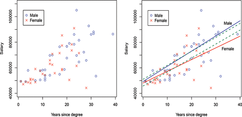
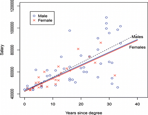
To illustrate the use of this model, take the following example. Suppose the data consist of those values for Y = Salary (in $'s) plotted in Figure 1(a) against the predictor variable X = Years since degree, or simply “years.” It is desired to fit a separate regression equation through each of the male and female data points. Thus, Equation (2(2) $$\begin{array}{ccc}\hfill Y& =& {\beta }_0+{\beta }_1{X}_1+\cdots +{\beta }_p{X}_p+{\beta }_{p+1}\text{gender}\hfill \\ & & +{\beta }_{p+2}{X}_1\times \text{gender}+\cdots +{\beta }_{2p+1}{X}_p\times \text{gender}+e.\hfill \end{array}$$(2) ) can be written as (3) $$\begin{array}{c}\hfill Y={\beta }_0+{\beta }_1\text{years}+{\beta }_2\text{gender}+{\beta }_3\text{gender}\times \text{years}+e.\end{array}$$(3) For these data, the regression equation becomes (4) $$\begin{array}{ccc}\hfill \widehat{Y}& =& 48134.0+917.2\text{years}+1189.4\text{gender}\hfill \\ & & +271.3\text{gender}\times \text{years,}\hfill \end{array}$$(4) where $\widehat{Y}$ is the predicted value of the response Y for given values of the regression variables. Substituting gender = 1 for males, into Equation (4(4) $$\begin{array}{ccc}\hfill \widehat{Y}& =& 48134.0+917.2\text{years}+1189.4\text{gender}\hfill \\ & & +271.3\text{gender}\times \text{years,}\hfill \end{array}$$(4) ), we obtain the male regression equation (5) $$\widehat{Y}=49323.4+1188.5\text{years};$$(5) and substituting gender = 0 for females, into Equation (4(4) $$\begin{array}{ccc}\hfill \widehat{Y}& =& 48134.0+917.2\text{years}+1189.4\text{gender}\hfill \\ & & +271.3\text{gender}\times \text{years,}\hfill \end{array}$$(4) ), we obtain the female regression equation (6) $$\widehat{Y}=48134.0+917.2\text{years}.$$(6)

Figure 1. Salary vs. years, left (a) raw data, right and (b) regression fits by gender—solid lines use indicator interactions and dashed lines do not use indicator interactions.

Note that these fits of Equations (5(5) $$\widehat{Y}=49323.4+1188.5\text{years};$$(5) ) and (6(6) $$\widehat{Y}=48134.0+917.2\text{years}.$$(6) ) were obtained by fitting Equation (3(3) $$\begin{array}{c}\hfill Y={\beta }_0+{\beta }_1\text{years}+{\beta }_2\text{gender}+{\beta }_3\text{gender}\times \text{years}+e.\end{array}$$(3) ) to all the observations (i.e., to the dataset containing both the male and female values). The intercept term (β₀ + β₂ for males and β₀ for females) represents a base, or starting salary; and the slope (β₁ + β₃ for males and β₁ for females) represents the yearly increase in $’s. If no gender inequity existed, then the estimates for the β₂ and β₃ parameters would be close to zero, producing male and female regressions that were not statistically significantly different from each other. In this case, however, Equations (5(5) $$\widehat{Y}=49323.4+1188.5\text{years};$$(5) ) and (6(6) $$\widehat{Y}=48134.0+917.2\text{years}.$$(6) ) are clearly different from each other, as are the divergent regression lines in Figure 1(b). A natural consequence of this widening gap is that with the inherent cumulative effect that results, females are increasingly disadvantaged over time.

Had we separately fitted the model (7) $$Y={\beta }_0+{\beta }_1\text{years}+e$$(7) to the dataset consisting of males only and the dataset consisting of females only, then the resulting equations are exactly the same as in Equations (5(5) $$\widehat{Y}=49323.4+1188.5\text{years};$$(5) ) and (6(6) $$\widehat{Y}=48134.0+917.2\text{years}.$$(6) ), for males and females, respectively, as they should be. The upper blue regression line of Figure 1(b) shows the fit of Equation (5(5) $$\widehat{Y}=49323.4+1188.5\text{years};$$(5) ) for males and the lower red regression line shows the fit of Equation (6(6) $$\widehat{Y}=48134.0+917.2\text{years}.$$(6) ) for females.

While there is a wealth of literature concerned with the study of salary inequities by gender, it is unfortunately the case that often times these studies fail to include the indicator interaction terms. Instead of the model of Equation (3(3) $$\begin{array}{c}\hfill Y={\beta }_0+{\beta }_1\text{years}+{\beta }_2\text{gender}+{\beta }_3\text{gender}\times \text{years}+e.\end{array}$$(3) ), these incorrectly use the model (8) $$Y={\beta }_0+{\beta }_1\text{years}+{\beta }_2\text{gender}+e.$$(8) For the data of Figure 1(a), the resulting regression equation from Equation (8(8) $$Y={\beta }_0+{\beta }_1\text{years}+{\beta }_2\text{gender}+e.$$(8) ) becomes (9) $$\widehat{Y}=46176.8+1064.7\text{years}+2205.9\text{gender}.$$(9) Substituting gender = 1 for males, into Equation (9(9) $$\widehat{Y}=46176.8+1064.7\text{years}+2205.9\text{gender}.$$(9) ), gives a male equation as (10) $$\widehat{Y}=48382.7+1064.7\text{years};$$(10) and substituting gender = 0 for females, into Equation (9(9) $$\widehat{Y}=46176.8+1064.7\text{years}+2205.9\text{gender}.$$(9) ), gives a female equation as (11) $$\widehat{Y}=46176.8+1064.7\text{years}.$$(11) Notice these two equations are parallel, as demonstrated by the green dashed lines in Figure 1(b).

These parallel equations could pertain when both males and females receive the same yearly raise in $’s. That is, Equations (10(10) $$\widehat{Y}=48382.7+1064.7\text{years};$$(10) ) and (11(11) $$\widehat{Y}=46176.8+1064.7\text{years}.$$(11) ), with their equal slopes, imply that the yearly salary increase in $’s is the same for males as for females, and so are unable to capture annual disparities in merit/productivity raises should they exist. Indeed, in this case, the raise amount (here, $1064.7) is a larger percentage of the female base (here, 2.306% = (1064.7/46176.8) × 100%) than it is for the male base (2.201% = (1064.7/48382.7) × 100%) which implies the females received a higher percentage annual raise on average than did the males.

If salary raises are based on productivity measures that are themselves biased against females (see Section 8), then with each passing year and average lower raises for females, the gender salary gap widens with the cumulative effect of these lower raises prevailing. Hence, the relevant regression equations need to reflect this phenomenon. In this case, it is the diverging regressions (of Equations (4(4) $$\begin{array}{ccc}\hfill \widehat{Y}& =& 48134.0+917.2\text{years}+1189.4\text{gender}\hfill \\ & & +271.3\text{gender}\times \text{years,}\hfill \end{array}$$(4) )–(6(6) $$\widehat{Y}=48134.0+917.2\text{years}.$$(6) )) that pertain, rather than the parallel equations (Equations (9(9) $$\widehat{Y}=46176.8+1064.7\text{years}+2205.9\text{gender}.$$(9) )–(11(11) $$\widehat{Y}=46176.8+1064.7\text{years}.$$(11) )).

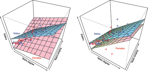
To illustrate briefly the use of two predictor variables, consider the predictor variables X₁ = years since degree (or, “degree”) and X₂ = years employed at current institution (or, “employ”). Then, Equation (1(1) $$Y={\beta }_0+{\beta }_1{X}_1+\cdots +{\beta }_p{X}_p+e,$$(1) ) becomes (12) $$\begin{array}{ccc}\hfill Y& =& {\beta }_0+{\beta }_1\text{degree}+{\beta }_2\text{employ}+{\beta }_3\text{gender}+{\beta }_4\text{gender}\hfill \\ & & \times \text{degree}+{\beta }_5\text{gender}\times \text{employ}+e.\hfill \end{array}$$(12) For these data, the regression equation becomes (13) $$\begin{array}{ccc}\hfill \widehat{Y}& =& 46773.0+581.3\text{degree}+755.4\text{employ}\hfill \\ & & -3085.0\text{gender}+2197.8\text{gender}\times \text{degree}\hfill \\ & & -2583.4\text{gender}\times \text{employ}.\hfill \end{array}$$(13) When the indicator by predictor interaction terms are omitted, we have (14) $$\begin{array}{ccc}\hfill \widehat{Y}& =& 44693.9+1507.2\text{degree}-569.9\text{employ}\hfill \\ & & +6098.7\text{gender}.\hfill \end{array}$$(14) Substituting gender = 1 for males and gender = 0 for females, we obtain the respective equations for males and females. Now, the regressions are planes in three-dimensional space. For the correct model of Equation (13(13) $$\begin{array}{ccc}\hfill \widehat{Y}& =& 46773.0+581.3\text{degree}+755.4\text{employ}\hfill \\ & & -3085.0\text{gender}+2197.8\text{gender}\times \text{degree}\hfill \\ & & -2583.4\text{gender}\times \text{employ}.\hfill \end{array}$$(13) ), these will be diverging planes, as shown in Figure 2(a), whereas for the incorrect model Equation (14(14) $$\begin{array}{ccc}\hfill \widehat{Y}& =& 44693.9+1507.2\text{degree}-569.9\text{employ}\hfill \\ & & +6098.7\text{gender}.\hfill \end{array}$$(14) ), these will be parallel planes as seen in Figure 2(b).

Figure 2. Data and regression surfaces for two predictors model, left (a) with indicator interactions, right (b) without indicator interactions.

Thus, if there are no gender inequities in yearly raises (in $’s), then the parallel equations evolving from Equation (9(9) $$\widehat{Y}=46176.8+1064.7\text{years}+2205.9\text{gender}.$$(9) ) or Equation (14(14) $$\begin{array}{ccc}\hfill \widehat{Y}& =& 44693.9+1507.2\text{degree}-569.9\text{employ}\hfill \\ & & +6098.7\text{gender}.\hfill \end{array}$$(14) ) could be valid. However, if the analysis is designed to identify inequities, then clearly this would not be an appropriate formulation as it presupposes no inequities. Existing inequities can only be identified by the model generated by Equation (3(3) $$\begin{array}{c}\hfill Y={\beta }_0+{\beta }_1\text{years}+{\beta }_2\text{gender}+{\beta }_3\text{gender}\times \text{years}+e.\end{array}$$(3) ) or Equation (12(12) $$\begin{array}{ccc}\hfill Y& =& {\beta }_0+{\beta }_1\text{degree}+{\beta }_2\text{employ}+{\beta }_3\text{gender}+{\beta }_4\text{gender}\hfill \\ & & \times \text{degree}+{\beta }_5\text{gender}\times \text{employ}+e.\hfill \end{array}$$(12) ), which produces the widening disparities that occur over time when inequities do in fact occur.

2.2. Looking at the Fits

The theory behind the calculation of the regression lines is that the estimates of the model parameters (the β_j, j = 0, 1, …, p, of Equation (1(1) $$Y={\beta }_0+{\beta }_1{X}_1+\cdots +{\beta }_p{X}_p+e,$$(1) )) are those values which minimize the sum of squares of the residuals, that is, for observations (Y_i, X_i1, …, X_ip), i = 1, …, n, we minimize (15) $$\begin{array}{ccc}\hfill \sum _{i=1}^n{\text{residual}}_i^2& \equiv & \sum _{i=1}^n{e}_i^2\hfill \\ & =& \sum _{i=1}^n{(Y_i-{\beta }_0-{\beta }_1{X}_{i1}-\cdots -{\beta }_p{X}_{ip})}^2,\hfill \end{array}$$(15) where e_i is the residual for the ith observation, i = 1, …, n. This minimization gives the “best” fitted regression equation through the observations.

For the data used in the one-predictor variable gender comparisons of Section 2.1 (Equations (3(3) $$\begin{array}{c}\hfill Y={\beta }_0+{\beta }_1\text{years}+{\beta }_2\text{gender}+{\beta }_3\text{gender}\times \text{years}+e.\end{array}$$(3) )–(11(11) $$\widehat{Y}=46176.8+1064.7\text{years}.$$(11) )), fitting the regression line Equation (6(6) $$\widehat{Y}=48134.0+917.2\text{years}.$$(6) ) through the female observations gives ∑_iresidual²_i = 2871.2 × 10⁵ ≡ R²₍₆₎, say. The corresponding value when fitting Equation (11(11) $$\widehat{Y}=46176.8+1064.7\text{years}.$$(11) ) through the female observations gives ∑_iresidual²_i = 2925.7 × 10⁵ ≡ R²₍₁₁₎, say. For the regression equations fitted through the male observations, we have R²₍₅₎ = 2802.7 × 10⁵ and R²₍₁₀₎ = 2810.2 × 10⁵ when fitting Equations (5(5) $$\widehat{Y}=49323.4+1188.5\text{years};$$(5) ) and (10(10) $$\widehat{Y}=48382.7+1064.7\text{years};$$(10) ), respectively. Clearly, for each of the male and female regressions, the sum of squared residuals for the incorrect regression equations is larger than that for the correct model. In other words, while intuitively, we can see from the parallel lines of Figure 1(b) that the model Equation (8(8) $$Y={\beta }_0+{\beta }_1\text{years}+{\beta }_2\text{gender}+e.$$(8) ) cannot be correct, these residual comparisons show numerically that using the model without the appropriate interaction terms is misleading.

It is clear from the two sets of fits in Figure 1(b) that omitting the interaction term in the model (the green dashed parallel lines) has the effect of drawing the male and female regression lines closer than they really should be, as years increase, with the result that it appears any inequity is smaller than it really is. The impact on female salaries is therefore particularly egregious for those who have been faculty for some time.

Another aspect of these fits involves so-called tests of coincidences where we want to see if the two regression equations, for males and females, respectively, are statistically significantly different from each other. This is not the same as (the t-test) testing whether any one model parameter is statistically different from zero. Rather this is (an F-test) testing whether all parameters collectively (or, a collective subset of parameters) are different for different values of the indicator model.¹ To achieve this, it is necessary to use the dataset with both male and female observations and to use the indicator equations as in Equation (2(2) $$\begin{array}{ccc}\hfill Y& =& {\beta }_0+{\beta }_1{X}_1+\cdots +{\beta }_p{X}_p+{\beta }_{p+1}\text{gender}\hfill \\ & & +{\beta }_{p+2}{X}_1\times \text{gender}+\cdots +{\beta }_{2p+1}{X}_p\times \text{gender}+e.\hfill \end{array}$$(2) ). To illustrate, consider the two-predictor variable example of Equation (13(13) $$\begin{array}{ccc}\hfill \widehat{Y}& =& 46773.0+581.3\text{degree}+755.4\text{employ}\hfill \\ & & -3085.0\text{gender}+2197.8\text{gender}\times \text{degree}\hfill \\ & & -2583.4\text{gender}\times \text{employ}.\hfill \end{array}$$(13) ). When we test for the effect of the interaction variables,² the resultant p-value is p = 0.0002. That is, there is a significant difference between the “full” model containing all five variables in Equation (13(13) $$\begin{array}{ccc}\hfill \widehat{Y}& =& 46773.0+581.3\text{degree}+755.4\text{employ}\hfill \\ & & -3085.0\text{gender}+2197.8\text{gender}\times \text{degree}\hfill \\ & & -2583.4\text{gender}\times \text{employ}.\hfill \end{array}$$(13) ) and the “reduced” model which omits the interaction variables. It is instructive perhaps to notice that when the focus is on the gender variable alone, we obtain p = 0.6423 which suggests gender per se is not significant. However, as we saw, it is the interaction of gender with the predictor variables which produces significant differences in the models. Had we used the model of Equation (14(14) $$\begin{array}{ccc}\hfill \widehat{Y}& =& 44693.9+1507.2\text{degree}-569.9\text{employ}\hfill \\ & & +6098.7\text{gender}.\hfill \end{array}$$(14) ), we obtain p = 0.0995 for the gender variable, and so we would have erroneously concluded there was no significant difference between the parallel male and female regression equations. Looking at the effect of including all the gender variables in Equation (13(13) $$\begin{array}{ccc}\hfill \widehat{Y}& =& 46773.0+581.3\text{degree}+755.4\text{employ}\hfill \\ & & -3085.0\text{gender}+2197.8\text{gender}\times \text{degree}\hfill \\ & & -2583.4\text{gender}\times \text{employ}.\hfill \end{array}$$(13) ) gives p = 0.0001. That is, all the gender variables, including their interaction terms, are collectively significant and should be included in the full model.

3. Adjustments

The next question is how to make adjustments to the female salaries so as to remove inequities identified by the two differing regression fits. What is clear from Figure 1(b) is that the male salaries are scattered around the male regression equation, as are the female salaries scattered around the female regression equation. The equations themselves represent the respective average male and female salaries for given years. It is recognized that below and above average salaries occur for all sorts of reasons (such as greater/smaller productivity levels, compression and inversion questions,³ different merit scores, etc.) for both males and females. Our issue here is not to resolve those reasons but to focus on departures due to apparent gender inequitable salaries only. As an aside, if the male regression equation is below that for females, then the male salaries should be adjusted; likewise, for other minority groups. For the purposes herein, we assume it is the female salaries that need adjustment.

Gray and Scott (1980) first established the importance of adopting across-the-board adjustments both legally and statistically. Later, the dangers of using a case-by-case approach were echoed by Ferree and McQuillan (1998). That is, it is important not to take a case-by-case approach as would apply, for example, if the female identified as observation #4 in Figure 3 were singled out for consideration. It could well be that the person #1 has been treated more inequitably when all factors are taken into account. Indeed, a detailed examination of a female’s record might well be construed as “discriminatory” if such an analysis were not conducted for all females and all men. It would also likely be somewhat difficult and time consuming to achieve an adequate summary of anyone’s work, particularly as this would require assembling relevant information (such as quantity and quality of publications, conference invitations, grants, student supervisions, etc.) for all predictor variables for all males and females in the unit under study. One such exercise is reported in Barsanti, Billard, and Anderson (1993), in an across-the-board detailed analysis of one college. However, the literature essentially concurs this would be a difficult exercise; see, for example, Haignere (2002). Therefore, as emphasised by Gray and Scott (1980), it is important that all females receive some across-the-board adjustment as a unit if gender inequities have been identified in their salaries.

Figure 3. Salary adjustments: left (a) AAUP; right (b) our recommendation.

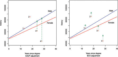
The AAUP recommendation, see Scott (1977), is to shift the female salaries that fall below the male regression equation up to the predicted value for a male with the same predictor variable characteristics. This is in effect the Peters (1941) and Belson (1956) approach. This is also sometimes referred to as the Blinder (1973) and Oaxaxa (1973) method; see, for example, Bura, Gastwirth, and Hikawa (2012), Jann (2008), and Graubard, Sowmya Rao, and Gastwirth (2005). In addition, Gastwirth (1989) considered this issue in a court setting concerned with minorities. A nice summary can be found in Sinclair and Pan (2009), who conclude with a recommendation that further scenarios be explored. One such approach is offered herein.

Figure 3 shows the regression fits for the data of Figure 1 and identifies four particular females for illustrative purposes. The implementation of the AAUP adjustment increases the salary of the two individuals, #3 and #4, to match the male salary, but it leaves the salaries of the individuals #1 and #2 unchanged; see Figure 3(a). When this is implemented for all females, we are left with a situation where no females have a salary below the male equation, but there still remain males with salaries below that line. This set-up, it seems, is unfair to those males with below average salaries, and it is also unfair to those females with above average salaries whose salaries are unchanged by this method.

Instead, based on Billard, Cooper, and Kaluba (1991, 1994), it is proposed here that adjustments be made as follows. The female regression line should be rotated so as to coincide with the male regression line, with the female salaries moved upward correspondingly. This is equivalent to adjusting the female salary by the amount equal to the difference between the predicted male salary and the predicted female salary, obtained from the respective regression equations, for the same predictor variables of each female. Formally, for the one-predictor variable case of Equation (3(3) $$\begin{array}{c}\hfill Y={\beta }_0+{\beta }_1\text{years}+{\beta }_2\text{gender}+{\beta }_3\text{gender}\times \text{years}+e.\end{array}$$(3) ) (multiple p predictor variables are handled similarly), we can write the predicted salary based on the male and female regressions, respectively, from Equation (3(3) $$\begin{array}{c}\hfill Y={\beta }_0+{\beta }_1\text{years}+{\beta }_2\text{gender}+{\beta }_3\text{gender}\times \text{years}+e.\end{array}$$(3) ), as (16) $${\widehat{Y}}_m=({\widehat{\beta }}_0+{\widehat{\beta }}_2)+({\widehat{\beta }}_1+{\widehat{\beta }}_3)\times \text{years},$$(16) (17) $${\widehat{Y}}_f={\widehat{\beta }}_0+{\widehat{\beta }}_1\times \text{years},$$(17) where ${\widehat{\beta }}_i,i=0,\cdots ,3$, are the regression parameters estimated from the data. Thus, for the data of Section 2.1, the adjustment for a female with a given value for years, ${\widehat{Y}}_m-{\widehat{Y}}_f$, becomes (18) $$\begin{array}{ccc}\hfill \text{Adjustment}& =& {\widehat{Y}}_m-{\widehat{Y}}_f={\widehat{\beta }}_2+{\widehat{\beta }}_3\times \text{years}\hfill \\ & =& 1189.4+271.3\times \text{years}.\hfill \end{array}$$(18)

Thus, for our four illustrative females in Figure 3, the adjusted salaries would be as shown in Figure 3(b). Such an adjustment procedure is fairer to all faculty in that unit including those males with below average salaries and to those females with above average salaries, in the following sense.

Salary increases through annual raises are typically made by an academic unit based on assessments of faculty productivity for a given period of time. This assessment can be made by a head/chair or a group/committee of senior faculty or the like, and productivity can be measured by a variety of activities such as publications, conference invitations, grants, and so on; and for the present purposes it is assumed the assessment time-frame is one year (though certainly such assessments could be for a rolling window of say two or more years). All else being equal, males with salaries above the male predicted regression equation (the blue line in Figure 3) have over the years received above average raises due to above average productivity levels compared to their male colleagues in the same unit; likewise, those whose salaries are below the regression equation have been relatively less productive. Similarly, females with salaries above (respectively, below) the female predicted regression equation (the red line in Figure 3) have been assessed as being more (respectively, less) productive than the other females in the unit.

By invoking the AAUP/Peters–Blinder approach (see Figure 3(a)), females with salaries below the male averages are increased to those male averages but males with salaries below the male average are left unchanged. This essentially takes no account of these females as having lower levels of productivity, while the males with lower average salaries retain salaries reflecting their lower levels of productivity. This then is not equitable for those males. By the same token in contrast, (the usually few in number) females with salaries above the male regression equation receive no adjustment by the AAUP method (again see observations #1, 2 in Figure 3(a)). Yet, these females have to have been exceptionally more productive not just compared to their female cohorts but even compared to the males in their unit to have such a relatively higher salary. To leave their salaries unadjusted would be quite unfair to such female faculty, especially if their higher productivity is not rewarded commensurately with their male highly productive counterparts who have been well rewarded with relatively higher salaries. The recommended adjusted method, by rotating the female (red line) regression to coincide with the male (blue line) regression, keeps the relative disparities of the salaries reflecting the cumulative productivity levels the same for both genders as they were before adjustment; that is, a female whose salary is $ S (say) more, or less, than the average predicted for her predictor values (here, years) still has the same $ S salary differential after adjustment. Clearly, the males also retain their respective relative salary differentials.

Since the female regression equation is typically below that for males, one consequence of this recommended adjustment procedure is that the average female adjustment tends to be lower than it might be when the AAUP adjustment method is implemented. For the data of Figure 1, the overall AAUP adjustment average is $6375 compared with our recommended adjustment average of $4789. An administrator might like this, but a female faculty might not. However, since justice and fairness for all faculty, male and female, should be the desired goal, we prefer this recommended adjustment.

A related issue deals with an administration’s response as to how to go forward from this point. Clearly, they are to be applauded for recognizing the legal and practical implications by making adjustments when salary inequities are identified. However, as, for example, Dempsey, Gillies, and Rietveld (2004) have reported, it is usually the case that, even after prior adjustments, gender inequities reemerge in salary levels. The reasons involve the broader issue of discrimination in general, and how women’s productivity measures and contributions are perceived compared to those of men. Gray and Scott (1980) delved into these murky waters. Unfortunately, the problems are still with us; Sandler (2000) explained that institutions still have a long way to go to achieve parity.

4. Comparisons by Disciplines

Including several disciplines into the one analysis can be conducted in the same manner as was done by including both genders. As in Section 2, both indicator variables for discipline and their interaction with predictor variables must be included in the model of Equation (3(3) $$\begin{array}{c}\hfill Y={\beta }_0+{\beta }_1\text{years}+{\beta }_2\text{gender}+{\beta }_3\text{gender}\times \text{years}+e.\end{array}$$(3) ), which now becomes, for p predictor variables, (19) $$\begin{array}{ccc}\hfill Y& =& {\beta }_0+{\beta }_1{X}_1+\cdots +\beta X_p+{\beta }_{p+1}\text{group}+{\beta }_{p+2}\text{group}\hfill \\ & & \times X_1+\cdots +{\beta }_{2p+1}\text{group}\times X_p+e,\hfill \end{array}$$(19) where a particular discipline here is identified by “group.”

This is illustrated for the data shown in Figure 4 where regression fits are made for two groups Group 1 and Group 2 and one predictor variable X₁ = X = years. In this case, Equation (19(19) $$\begin{array}{ccc}\hfill Y& =& {\beta }_0+{\beta }_1{X}_1+\cdots +\beta X_p+{\beta }_{p+1}\text{group}+{\beta }_{p+2}\text{group}\hfill \\ & & \times X_1+\cdots +{\beta }_{2p+1}\text{group}\times X_p+e,\hfill \end{array}$$(19) ) becomes, for one predictor variable years since degree, (20) $$\begin{array}{ccc}\hfill \widehat{Y}& =& 40496.8+1741.2\text{years}+3063.2\text{group}\hfill \\ & & +1267.9\text{group}\times \text{years}.\hfill \end{array}$$(20) When group = 1 is substituted, Equation (20(20) $$\begin{array}{ccc}\hfill \widehat{Y}& =& 40496.8+1741.2\text{years}+3063.2\text{group}\hfill \\ & & +1267.9\text{group}\times \text{years}.\hfill \end{array}$$(20) ) becomes (21) $$\widehat{Y}=43560.0+3009.1\text{years}$$(21) for Group 1; and when group = 0 is substituted, Equation (20(20) $$\begin{array}{ccc}\hfill \widehat{Y}& =& 40496.8+1741.2\text{years}+3063.2\text{group}\hfill \\ & & +1267.9\text{group}\times \text{years}.\hfill \end{array}$$(20) ) becomes, for Group 2, (22) $$\widehat{Y}=40496.8+1741.2\text{years}.$$(22) Were the regression model of Equation (7(7) $$Y={\beta }_0+{\beta }_1\text{years}+e$$(7) ) fitted to the Group 1 data alone, then the resulting equation is exactly as in Equation (21(21) $$\widehat{Y}=43560.0+3009.1\text{years}$$(21) ); likewise, Equation (22(22) $$\widehat{Y}=40496.8+1741.2\text{years}.$$(22) ) is the fitted equation when using the Group 2 data alone.

Figure 4. Comparing Group 1 and Group 2: solid lines use indicator interactions and dashed lines do not use indicator interactions.

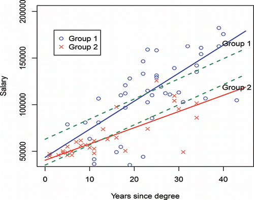
The intercept term (β₀) in each model essentially reflects different base or starting salaries for each discipline, with the regression slope parameter reflecting the average $ raise per year. Fits of these equations to these two groups are displayed in Figure 4, the upper blue line corresponding to Group 1 and the lower red line to Group 2.

When the indicator by predictor interaction terms are omitted from the model, Equation (19(19) $$\begin{array}{ccc}\hfill Y& =& {\beta }_0+{\beta }_1{X}_1+\cdots +\beta X_p+{\beta }_{p+1}\text{group}+{\beta }_{p+2}\text{group}\hfill \\ & & \times X_1+\cdots +{\beta }_{2p+1}\text{group}\times X_p+e,\hfill \end{array}$$(19) ) becomes (23) $$Y={\beta }_0+{\beta }_1{X}_1+\cdots +{\beta }_p{X}_p+{\beta }_{p+1}\text{group}+e.$$(23) For the data of Group 1 and Group 2, the resulting equation is (24) $$\widehat{Y}=35226.6+2158.6\text{years}+27742.0\text{group}.$$(24) Substituting group =1 gives, for Group 1, (25) $$\widehat{Y}=62968.6+2158.6\text{years};$$(25) and substituting group = 0 gives, for Group 2, (26) $$\widehat{Y}=35226.6+2158.6\text{years}.$$(26)

These^{Figure 5}two equations are parallel (see the green dashed lines of Figure 4). Notice in particular this implies each group has the same average increase in salary in $'s (here, 2158.6) each year. For those institutions which provide the same (or, approximately the same) average percentage yearly increases to groups (for allocation to individuals within a group), any regression model which determines equal $ average raises for all groups, as in Equations (24(24) $$\widehat{Y}=35226.6+2158.6\text{years}+27742.0\text{group}.$$(24) )–(26(26) $$\widehat{Y}=35226.6+2158.6\text{years}.$$(26) ), cannot represent the fact that years in service might be compensated differently (in $’s) in the two groups. An equation such as Equation (24(24) $$\widehat{Y}=35226.6+2158.6\text{years}+27742.0\text{group}.$$(24) ) can only be correct if both groups had the same average annual increments in $’s. This is usually not the case in an academic setting. For example, law salaries differ substantially from those for history. A comparison of the relative salary levels across disciplines from 1980 to 2010 can be found in, for example, Academe (2011, Tables G and H) which demonstrates these salary differences by discipline.

When there are more than two groups, Equation (19(19) $$\begin{array}{ccc}\hfill Y& =& {\beta }_0+{\beta }_1{X}_1+\cdots +\beta X_p+{\beta }_{p+1}\text{group}+{\beta }_{p+2}\text{group}\hfill \\ & & \times X_1+\cdots +{\beta }_{2p+1}\text{group}\times X_p+e,\hfill \end{array}$$(19) ) becomes the model (27) $$\begin{array}{ccc}\hfill Y& =& {\beta }_0+{\beta }_{1}X+{\beta }_2{\text{group}}_1+\cdots +{\beta }_g{\text{group}}_{g-1}+{\beta }_{g+1}{\text{group}}_1\hfill \\ & & \times X+\cdots +{\beta }_{2g-1}{\text{group}}_{g-1}\times X+e,\hfill \end{array}$$(27) where we have assumed, for illustrative purposes, that there is only one predictor variable X (such as years). Note there is one less group indicator variable than there are groups; this accommodates the last group Group g as having all zero values for the actual group indicator variables used.

We illustrate this with the raw data shown in Figure 5(a) for three groups. Here, a third Group 3 is added to the two groups Group 1 and Group 2 above. The resulting regression model is (28) $$\begin{array}{ccc}\hfill \widehat{Y}& =& 43131.6+1018.7\text{years}+428.4{\text{group}}_1-2634.8{\text{group}}_2\hfill \\ & & +1990.4{\text{group}}_1\times \text{years}+722.5{\text{group}}_2\times \text{years}.\hfill \end{array}$$(28) Thus, when the indicators group₁ = 1 and group₂ = 0, Equation (28(28) $$\begin{array}{ccc}\hfill \widehat{Y}& =& 43131.6+1018.7\text{years}+428.4{\text{group}}_1-2634.8{\text{group}}_2\hfill \\ & & +1990.4{\text{group}}_1\times \text{years}+722.5{\text{group}}_2\times \text{years}.\hfill \end{array}$$(28) ) becomes, for Group 1, (29) $$\widehat{Y}=43560.0+3009.1\text{years};$$(29) when the indicators group₁ = 0 and group₂ = 1, Equation (28(28) $$\begin{array}{ccc}\hfill \widehat{Y}& =& 43131.6+1018.7\text{years}+428.4{\text{group}}_1-2634.8{\text{group}}_2\hfill \\ & & +1990.4{\text{group}}_1\times \text{years}+722.5{\text{group}}_2\times \text{years}.\hfill \end{array}$$(28) ) becomes, for Group 2, (30) $$\widehat{Y}=40469.8+1741.2\text{years};$$(30) and when the indicators group₁ = 0 and group₂ = 0, Equation (28(28) $$\begin{array}{ccc}\hfill \widehat{Y}& =& 43131.6+1018.7\text{years}+428.4{\text{group}}_1-2634.8{\text{group}}_2\hfill \\ & & +1990.4{\text{group}}_1\times \text{years}+722.5{\text{group}}_2\times \text{years}.\hfill \end{array}$$(28) ) becomes, for Group 3, (31) $$\widehat{Y}=43131.6+1018.7\text{years}.$$(31) Notice that Equations (29(29) $$\widehat{Y}=43560.0+3009.1\text{years};$$(29) ) and (30(30) $$\widehat{Y}=40469.8+1741.2\text{years};$$(30) ) for Group 1 and Group 2 are the same as those calculated in Equations (21(21) $$\widehat{Y}=43560.0+3009.1\text{years}$$(21) ) and (22(22) $$\widehat{Y}=40496.8+1741.2\text{years}.$$(22) ) for these same two groups, respectively. The regression plots for these three groups are displayed in Figure 5(b).

Figure 5. Groups 1–3: left (a) raw data; right (b) regression fits by group.

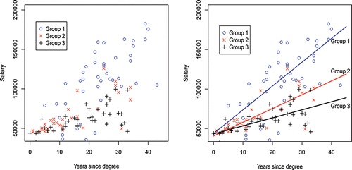
Again, omission of the different group × X interaction terms produces three parallel lines which are clearly incorrect regression equations, unless all groups have the same salary structure which is unlikely, for example, salaries for law, history and biology are quite different from each other.

5. Grouping Disciplines

When sample sizes for gender or disciplinary groups are small (evidenced by large standard deviations for the regression parameters), it might be beneficial to merge units to reach suitable sample sizes for the analyses to be valid.⁴ If the number of observations is too small, then conclusions drawn by the t-tests or F-tests in fitting the regression models have insufficient power. Care is needed when merging units however, as any resulting group should be formed from units that have a similar salary structure.

It is reasonably easy to test for normality of the underlying dataset (e.g., in SAS, invoke “proc univariate data=<name of data-set> normal; var salary; run;”). Four tests for normality are the default (viz., Shapiro–Wilk, Kolmogorov–Smirnov, Cram$\acute{e}$r–von Mises, and Anderson–Darling tests; the specific details are not important to the present discussion).

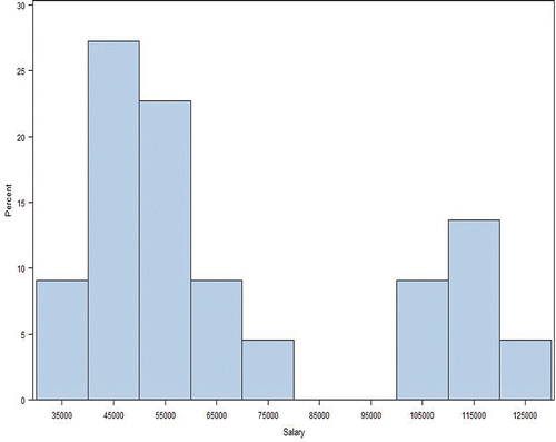
For example, consider two units Group 1 and Group 2, say. Separately each group has a salary structure that is normally distributed. However, when merged into one group, we find that the male salaries of this merged group are normally distributed; but the salaries of the females are not at all normally distributed. In fact, the female salary structure is quite bi-modal, as demonstrated in Figure 6; here, the histogram of the salaries of the Group 1 females is to the left centered around 51,000 whereas the histogram for salaries of Group 2 females lies to the right centered around 115,000. Since the number of females in each of these groups is small, a more suitable grouping has to be found to study gender salary differentials for these individuals.⁵

Figure 6. Bimodal histogram for merged Group 1 and Group 2 females.

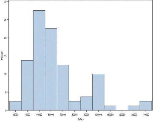
In this particular case, merging Group 1 with a different group, Group 3, is more suitable. The combined histogram plots for this grouping for female and male salaries are shown in Figures 7 and 8, respectively. The normality test results are confirmed.

Figure 7. Normal histogram for merged Group 1 and Group 3 females.

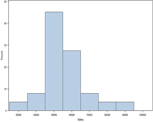
Figure 8. Normal histogram for merged Group 1 and Group 3 males.

6. Outliers

Another issue relates to outlier observations. Consider again the combined Group 1 and Group 3 male salaries, in particular the histogram of male salaries shown in Figure 8. There appear to be outlier salaries above 125,000. On even further inspection, one of these observations relates to a salary for a male with a very high value for the predictor variable, years. On further investigation, his salary is well within two standard deviations of the predicted salary for someone with his years. Therefore, this observation should be retained in any analysis. On the other hand, the other observations for which the salary >125,000 are outside the two standard deviation range for their respective years, and so are real outliers. A detailed investigation of the influence of outliers has been made by Cook and his colleagues, see, for example, Thomas and Cook (1989, 1990); we omit that discussion here. It is also important that any process to exclude outliers be such that it does not provide an opportunity for bias to intrude.

The effect of including these outliers in the analysis is shown by the upper dotted regression line in Figure 9. The male regression line obtained by ignoring the outliers is the heavy blue line in Figure 9, and the female regression fit is the heavy red line of Figure 9. Clearly, in this case, by ignoring outliers, it would seem that there is no gender salary inequity between the males and females of this grouping (Group 1 and Group 3 combined).

Figure 9. Regression fits by gender for merged Group 1 and Group 3. Upper dashed line for males includes two outliers.

The difference between the two fitted regression lines for male salaries raises another issue that frequently prevails. When outliers do occur, it behooves the institution to take a careful look at them and the conditions which produced them, even if only to assure themselves that they are not unwittingly perpetuating discrimination. Occasionally, there are easily identified outlier salaries that evolved from a faculty member having received a truly outstanding recognition such as a Nobel Prize. This is not something to which any given faculty member generally might aspire. More frequently, an institution will reward high-flying faculty with large substantial salary adjustments in response to their being awarded some prestigious recognition or election to a prestigious professional society presidency and the like. It is not unexpected that such faculty have exceptionally high salaries. However, if male high-flyers are rewarded and female high-flyers are not so rewarded, then there is an inherent inequity to the salaries of those females. Often however, there might be relatively high male salaries (even ones identified as outliers) because of current or prior appointments to administrative positions such as department heads/chairs or directors of centers. When more males than females serve in these positions, there results a built-in bias against female faculty with a commensurate relative negative effect on salary. There is also again, perhaps inadvertently, inequity if the salaries of women who are appointed to such positions are not upgraded to the same extent as for males when they are appointed. Outliers, or “lower-level” outliers such as these, can exist for all sorts of reasons, and should be handled carefully and in a way that is not itself discriminatory.

If there is true gender equity, then there should also be some female high salaries. Therefore, if outliers exist for male salaries but not for female salaries, to help redress those difficulties, it can be argued that it is the equation obtained by the full set of male salaries (the dotted line of Figure 9) that should be used when making adjustments to the female salaries (see Section 3). Indeed, Gastwirth (1988) discussed a court case that argued that these outliers should be included even though the higher male salaries related to prior administrative duties.

7. Gender and Discipline Indicators

As intimated in Section 4, it is well known that different disciplines experience different average salary structures. An omnibus model can involve both discipline and gender differences. In the same way that indicator variables are used for gender (see Section 2) and for discipline or groups (see Section 4), indicator variables for both gender and groups can be inserted into the same regression analyses. Again, care must be taken to include the indicator by predictor interaction terms. These interaction terms must also include indicator interaction terms. These principles are illustrated in the following example.

The dataset consists of the salaries and the predictor variable years, for males and females in two disciplines Group 4 and Group 5 and are displayed in Figure 10. The regression model of Equation (1(1) $$Y={\beta }_0+{\beta }_1{X}_1+\cdots +{\beta }_p{X}_p+e,$$(1) ) becomes, by combining the principles of Equations (2(2) $$\begin{array}{ccc}\hfill Y& =& {\beta }_0+{\beta }_1{X}_1+\cdots +{\beta }_p{X}_p+{\beta }_{p+1}\text{gender}\hfill \\ & & +{\beta }_{p+2}{X}_1\times \text{gender}+\cdots +{\beta }_{2p+1}{X}_p\times \text{gender}+e.\hfill \end{array}$$(2) ) and (19(19) $$\begin{array}{ccc}\hfill Y& =& {\beta }_0+{\beta }_1{X}_1+\cdots +\beta X_p+{\beta }_{p+1}\text{group}+{\beta }_{p+2}\text{group}\hfill \\ & & \times X_1+\cdots +{\beta }_{2p+1}\text{group}\times X_p+e,\hfill \end{array}$$(19) ), for one predictor variable years, (32) $$\begin{array}{ccc}\hfill Y& =& {\beta }_0+{\beta }_1\text{years}+{\beta }_2\text{gender}+{\beta }_3\text{gender}\times \text{years}\hfill \\ & & +{\beta }_4\text{group}+{\beta }_5\text{group}\times \text{years}+{\beta }_6\text{gender}\times \text{group}\hfill \\ & & +{\beta }_7\text{gender}\times \text{group}\times \text{years}+e.\hfill \end{array}$$(32)

Figure 10. Groups 4 and Group 5: regression fits by gender and group left (a) correct regressions; right (b) incorrect regressions—yellow and green lines (for Group 4) and blue and red lines (for Group 5) represent the male and female regressions, respectively.

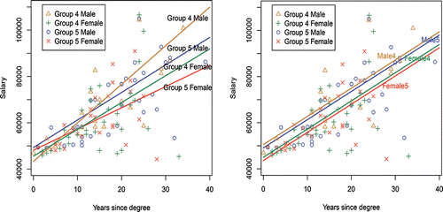
For the data of Figure 10, the fitted model is (33) $$\begin{array}{ccc}\hfill \widehat{Y}& =& 48134.0+917.2\text{years}+1189.4\text{gender}+271.3\text{gender}\hfill \\ & & \times \text{years}-2550.7\text{group}+241.0\text{group}\times \text{years}\hfill \\ & & -3446.5\text{gender}\times \text{group}+234.7\text{gender}\times \text{group}\hfill \\ & & \times \text{years}.\hfill \end{array}$$(33) Substituting group = 1 for Group 4, and gender = 1, 0 for males and females, respectively, into Equation (33(33) $$\begin{array}{ccc}\hfill \widehat{Y}& =& 48134.0+917.2\text{years}+1189.4\text{gender}+271.3\text{gender}\hfill \\ & & \times \text{years}-2550.7\text{group}+241.0\text{group}\times \text{years}\hfill \\ & & -3446.5\text{gender}\times \text{group}+234.7\text{gender}\times \text{group}\hfill \\ & & \times \text{years}.\hfill \end{array}$$(33) ), we obtain (34) $$\begin{array}{ccc}\hfill \widehat{Y}& =& 43326.2+1664.2\text{years}\hfill \end{array}$$(34) and (35) $$\begin{array}{ccc}\hfill \widehat{Y}& =& 45583.3+1158.2\text{years}\hfill \end{array}$$(35) as the male and female regression equations, respectively. Likewise, substituting group = 0 for Group 5, and gender = 1, 0 for males and females, respectively, into Equation (33(33) $$\begin{array}{ccc}\hfill \widehat{Y}& =& 48134.0+917.2\text{years}+1189.4\text{gender}+271.3\text{gender}\hfill \\ & & \times \text{years}-2550.7\text{group}+241.0\text{group}\times \text{years}\hfill \\ & & -3446.5\text{gender}\times \text{group}+234.7\text{gender}\times \text{group}\hfill \\ & & \times \text{years}.\hfill \end{array}$$(33) ), gives (36) $$\begin{array}{ccc}\hfill \widehat{Y}& =& 49323.4+1188.5\text{years}\hfill \end{array}$$(36) and (37) $$\begin{array}{ccc}\hfill \widehat{Y}& =& 48134.0+917.2\text{years}\hfill \end{array}$$(37) as the male and female regression equations, respectively. As an aside, this Group 5 happens to be the same academic grouping used in the gender discussion in Section 2; therefore, the regressions here of Equations (36(36) $$\begin{array}{ccc}\hfill \widehat{Y}& =& 49323.4+1188.5\text{years}\hfill \end{array}$$(36) ) and (37(37) $$\begin{array}{ccc}\hfill \widehat{Y}& =& 48134.0+917.2\text{years}\hfill \end{array}$$(37) ) are identical to those calculated in Equations (5(5) $$\widehat{Y}=49323.4+1188.5\text{years};$$(5) ) and (6(6) $$\widehat{Y}=48134.0+917.2\text{years}.$$(6) ). These regression lines are shown in Figure 10(a). As is customary in academia, the group regressions widen as years increase, reflecting different salary scales by different disciplines. When male and female salaries within a given discipline (group) diverge, there is evidence of salary inequities by gender.

If the indicator interaction terms are omitted from the model, these data produce the equation (38) $$\begin{array}{ccc}\hfill \widehat{Y}& =& 43451.2+1222.6\text{years}+5515.1\text{gender}\hfill \\ & & +1428.6\text{group}.\hfill \end{array}$$(38) Setting group = 1 for Group 4, and gender = 1, 0 for males and females, into Equation (38(38) $$\begin{array}{ccc}\hfill \widehat{Y}& =& 43451.2+1222.6\text{years}+5515.1\text{gender}\hfill \\ & & +1428.6\text{group}.\hfill \end{array}$$(38) ), produces (39) $$\begin{array}{ccc}\hfill \widehat{Y}& =& 50524.9+1222.6\text{years},\text{and}Y=45009.8\hfill \\ & & +1222.6\text{years}\hfill \end{array}$$(39) as the male and female respective fits; and likewise, with group = 0 for Group 5, we obtain, from Equation (38(38) $$\begin{array}{ccc}\hfill \widehat{Y}& =& 43451.2+1222.6\text{years}+5515.1\text{gender}\hfill \\ & & +1428.6\text{group}.\hfill \end{array}$$(38) ), (40) $$\begin{array}{ccc}\hfill \widehat{Y}& =& 49096.2+1222.6\text{years},\text{and}Y=43581.2\hfill \\ & & +1222.6\text{years}\hfill \end{array}$$(40) as the male and female respective fits. These fits are shown in Figure 10(b). As was evident in the discussions in Sections 2 and 4, these are parallel lines, representing equal $ salary increases each year. This phenomenon is clearly inaccurate for different disciplines and different genders unless both disciplines and/or both genders have the same starting salaries and receive the same average increases in $’s per year, which factor hardly prevails in academic environments (see, e.g., Academe 2011).

8. Predictor Variables

The literature is replete with studies on salary inequity issues. Most of these are either reviews of other studies and/or reporting on the results at some specific institution. Almost all use the multiple regression model of Equation (1(1) $$Y={\beta }_0+{\beta }_1{X}_1+\cdots +{\beta }_p{X}_p+e,$$(1) ) in some form or another. All deal with their choices of predictor variables to use in their study.

A common thread is the standard choice of years since the doctoral degree (corresponding to the X ≡ X₁ variable used earlier in Sections 2, 4, and 7). Rather than doctorate degree, the degree may be an appropriate “highest” degree credential, such as a Masters of Fine Arts, or a Doctor of Veterinary Medicine.

A predictor variable variously described as “experience” representing years employed is often included. This frequently appears as years employed at current institution as information on years employed at previous institutions may be difficult to ascertain. Occasionally, this is estimated by versions of current year minus degree year; however, this could be comparable to the years since degree variable and so would be redundant. Also, how to account for years not served in faculty ranks may be difficult to assess. Such questions clearly need further study. However, it may be defined, studies usually use this experience variable as a linear predictor though some also add a squared experience term to their model on the grounds that compression and declining productivity with age are factors affecting faculty salaries (e.g., Moore, Newman, and Turnbull 1998; Brown and Woodbury 1998; Bratsberg, Ragan, and Warren 2003).

8.1. Rank

Use of rank as a predictor variable is contentious and controversial at best; Haignere (2002) referred to this as the “most hotly debated” issue. Where used, it tends to be used as a proxy for unavailable productivity variables. The AAUP, Scott (1977), is clear when it says “rank (and tenure) should not be employed as predictor variables of salary” especially since their use will underestimate any inequity that might exist. Scott (1977) elucidated how these entities are so closely related, especially when, as is usually the case, it is the same unit, same faculty, making both promotion and salary decisions.

While not the purview of the present article to make a definitive study, it is well documented that it is harder for women to publish than it is for men (though this can be mitigated if double-blind reviewing predominates); see, for example, Eagly and Carli (2003) and the Goldberg (1968) paradigm, Sandler (1986), and Jagsi et al. (2006). Often forgotten in this debate is the pervasive effect on teaching evaluations where female faculty are judged by higher standards in the classroom than are male instructors (see, e.g., the discussion in Laube et al. 2007). Gray (1993) has an extensive detailed review of what types of difficulties are encountered when trying to assign measures to productivity entities. That is, the underlying difficulty here is that rank and productivity measures are themselves gender-biased, or “tainted” variables. There is a universal acceptance that tainted or biased variables should not be used in salary regression analyses, as they underestimate the level of inequity; see, for example, Luna (2006), Johnson, Riggs, and Downey (1987), Barbezat (1991, 2002). Indeed, Finkelstein (1980), who coined the term, in his review of the judicial responses to these models is adamant that “If there has been discrimination in promotions, salary is likely to be a tainted variable, the effect of its inclusion being to conceal discrimination with respect to awards of salary.” As earlier suggested by Scott (1977), Finkelstein (1980) concurred that “including rank as an explanatory variable could incorrectly explain away discrimination in salary even if the differences between men and women with respect to awards of rank were not statistically significant.”

Nevertheless, the intuitive appeal to use rank and time in rank in lieu of productivity is strong. Several studies, by using a variety of datasets, consider models which do, and do not, include a rank variable; see, for example, Hoffman (1976), Barbezat (1991), Toutkoushian and Conley (2005), and Boudreau et al. (1997). In all cases, when rank was included, apparent salary inequities were reduced, thus corroborating the warning of the earlier AAUP conclusions in Scott (1977) and Finkelstein (1980) against the use of rank.

The AAUP study reported by Haignere (2002) sums up these sentiments best by asserting that those who control rank also control salaries, so if bias exists in one it exists in the other. Haignere (2002) said that if rank is to be used as a predictor variable, then performance measures should also be used to assess its appropriateness, further adding that it is unwieldly if not impossible to collect such data, and so elected not to collect performance data in their studies. This circles us back to the original AAUP study of Scott (1977) which demonstrated that within a given institution and discipline, since productivity measures are relatively homogeneously defined, adding productivity measures even if easily attainable adds little to the predictor equations.

Actual studies on ascertaining whether or not rank is itself gender biased are hard to achieve, primarily because of the difficulties in assessing productivity measures to compare performances. One study by Smart (1991) showed that rank was gender related. The Johnson, Riggs, and Downey (1987) study observed that predicted levels of tenure and rank for women were higher than those actually achieved. They suggested that these predicted values should be used as the predictor variables if the analyst wants to use rank in the regression model; the reader is cautioned however of the need to account for the variability of the predicted rank and that often the same variables are used as in the salary regression model with the effect that adding the predicted ranks may not add any additional information. Toutkoushian (1999) documented how this rank bias still persists. Euben (2001) reported on a case which showed a considerable gap (7.38 years longer in lower ranks) in promotion for females. An editorial on the slowness of promotions for women is in Shaw (2007).

Perceptions are that such disparities no longer exist. Unfortunately, as seen from Figure 11 (an updated version of Figure 4 in Billard and Kafadar 2015), the percentage differential between men and women who have been awarded tenure is unchanged since 1972, the year that Title IX became law. This disparity with tenure relates at least to some extent with promotion out of the Assistant Professor rank. Figure 12 shows the percentage of males and of females at each of the Full Professor, Associate Professor and Assistant Professor ranks. From the (a) plots (full blue lines) in Figure 12, we observe that, as for tenure, there is an approximately constant percentage differential between men and women, with an average of 46% of men and 21% for females at the Full Professor level over the years 1994–2015. Further, in contrast, from the corresponding (c) plots (dashed red lines) for the Assistant Professors, the percentage of females in the Assistant Professor rank is higher than that for males (averages of 31% and 20%, respectively); and while the percentage gap (dot-dash-dot green (b) lines) at the Associate Professor level is narrower (28% and 26% for females and males, respectively), it is clear from the (b) and (c) plots in Figure 12 that these gaps have persisted for the last twenty years. These observations are for Category I doctoral institutions as published annually in Academe.

Figure 11. Percent tenure rates by gender.

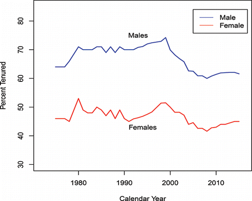
Figure 12. Percentage male and female by rank.

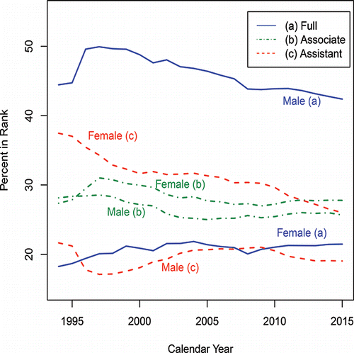
Whatever caveats may be imposed upon these data, there is no avoiding the conclusion that females are still not moving up the ranks as fast as males are. Earlier arguments that females have not been in the pipelines long enough to achieve the fruits of promotion are no longer germane. Indeed, West and Curtis (2006) concurred that this “ceiling remains most rigid” and that “inequities persist in the career progression of faculty women.” That is, rank continues to be a gender-biased tainted variable.

As a separate issue, since, as these data suggest, females are staying in the lower ranks longer than males are, it is important for institutions to undertake critically directed studies seeking ways to ask why the females at their particular institution are not being equitably promoted. Pragmatic approaches are needed. Gray and Scott (1980) discussed at length ways to address this issue. They also explain why it is so difficult to conduct gender-free biases when studying productivity entities, which entrenched difficulties no doubt help explain why these inequities in rank and salary persist still today. Unfortunately, these biases have a propensity to creep in no matter how hard institutions try to avoid them. Indeed, as Handelsman et al. (2005) summarized, removal of these invisible biases will take a concerted effect by an entire administration.

8.2. Beware of Collinearity

Collinearity can occur when two or more predictor variables indirectly contribute the same information to the prediction of the response dependent variable (Y). Little attention seems to have been given to the question of collinearity among the choices of predictor variables, despite the fact that several of the variables used would intuitively seem to be highly correlated. Luna (2006) suggested collinearity problems were insufficient to undermine a legal case being reviewed. Earlier, Billard, Cooper, and Kaluba (1994) showed that for a particular dataset, the use of one or both of the predictor variables, X₁ = years since degree and X₂ = years employed at the current institution, produced very similar predictions. Obtaining total years in the employment sector can be problematical. One solution has been the use of surrogate years employed such as years elapsed since the doctoral degree; however this measure is clearly correlated to the years since degree variable and so it is advisable to avoid this usage. Moore (1993) opined the effect of collinearity is minimal.

9. Conclusion

This study is an expansion of an earlier report by Billard, Cooper, and Kaluba (1994). It would have been hoped that by now analytical issues would no longer be an issue. As Sandler (2000) said at the conclusion of her history of the enactment of Title IX, “the struggle for educational equity is by no means over.” One aspect of this problem is the failure to use statistically adequate regression models when attempting to study salary levels. Unfortunately, too often, incorrect models are still used in too many analyses, even though they may be accepted by the courts, albeit erroneously. The most glaring error is the omission of the indicator interaction terms, whether these be indicators for gender and/or for discipline, or even rank. As has been illustrated in Sections 2, 4, and 7, failure to use a statistically correct formulation for the model results in parallel regression lines, which lines make any inequities between genders (and/or disciplines) seem smaller than they really are. These are scientific errors.

Other regression models may be more applicable for some data, such as logistic regression models (e.g., Fairlie 2005; Hikawa, Bura, and Gastwirth 2010), nonlinear regression models (e.g., Sinning, Hahn, and Bauer 2008), survival analysis ideas (Pan and Gastwirth 2005), or spline models (in which the overall regression consists of fits by components across subsets of the predictor variables; see, e.g., Wahba 1990). The principles described in the present article still pertain. In particular, it is important to include the indicator interaction terms; and adjustments to salary as suggested in Equation (18(18) $$\begin{array}{ccc}\hfill \text{Adjustment}& =& {\widehat{Y}}_m-{\widehat{Y}}_f={\widehat{\beta }}_2+{\widehat{\beta }}_3\times \text{years}\hfill \\ & =& 1189.4+271.3\times \text{years}.\hfill \end{array}$$(18) ), $\text{Adjustment}={\widehat{Y}}_m-{\widehat{Y}}_f$, still apply but where now the predicted male ${\widehat{Y}}_m$ salary and female salary ${\widehat{Y}}_f$ are calculated from the obtained fitted model/s.

Other components of the regression models may be more along philosophical lines, such as debates over which particular predictor variables should, or should not, be included in the model.

Comment: The datasets used in these analyses are based on actual datasets, from years past. However, the salary values per se have been transformed so that no one individual or unit can be identified. Some observations, such as outliers, have also been omitted. However, for the Group 1/3 analysis (see Figure 9), some outliers were included so as to illustrate their influence in an analysis. Finally, these analyses were done using the SAS and R packages.

Notes

1 This is easily tested in many regression packages, for example, in SAS, add the instruction “test < list of predictor variables>;”  when using the “proc reg” regression procedure.

2 Use “test gender ×degree, gender×employ.”

3 “Compression” and “inversion” occur when starting salaries are increasing faster than are merit raise increases; for “compression,” the lower ranked faculty person still has a salary lower than the longer serving faculty but the gap is shrinking, while “inversion” occurs when the starting salary has surpassed the salary of longer serving current faculty.

4 The often-used “rule of thumb” is to have about five times as many observations as there are predictor variables in the model; some authors, for example, Neter, Wasserman, and Kutner (1992) suggested 6 to 10.

5 As an aside, we caution that it could be that the two “groups” in Figure 6 may refer to some individuals who have fewer years and another group who have served many years so that these apparent differences merely reflect differences in longevity. The regression diagnostics should inform as to whether these differences are because of a non normality merging or simply because of longevity differences.

References

- Academic (2011), “It’s Not Over Yet, The Annual Report on the Economic Status of the Profession 2010–2011,” Academe, 97, 4–36.
- Barbezat, D. A. (1991), “Updating Estimates of Male-Female Salary Differentials in the Academic Labor Market,” Economic Letters, 36, 191–195.
- ——— (2002), “History of Pay Equity Studies,” New Directions for Institutional Research, 115, 9–39.
- Barsanti, J. A., Billard, L., and Anderson, D. P. (1993), “Gender Bias in Veterinary College Faculty Salaries? One University’s Approach,” Journal of Veterinary Medicine Education, 20, 45–49.
- Belson, W. A. (1956), “A Technique for Studying the Effects of a Television Broadcast,” Applied Statistics, 5, 195–202.
- Billard, L, Cooper, T. R., and Kaluba, J. A. (1991), “A Statistical Remedy to Gender and Race Based Salary Inequities,” Technical Report, University of Georgia.
- ——— (1994), “A Statistical Adjustment to Gender and Race Based Salary Inequities,” Technical Report, University of Georgia.
- Billard, L., and Kafadar, K. (2015), “Women in Statistics: Scientific Contributions Versus Rewards,” in Advancing Women in Science, eds. W. Pearson Jr., L. M. Frehill, and C. L. McNeely, New York: Springer, 201–214, 233.
- Blinder, A. S. (1973), “Wage Discrimination: Reduced Form and Structural Estimates,” Journal of Human Resources, 8, 436–455.
- Boudreau, N., Sullivan, J., Balzer, W., Ryan, A. M., Yonker, R., Thorsteinson, T., and Hutchinson, P. (1997), “Should Faculty Rank Be Included as a Predictor Variable in Studies of Gender Equity in University Faculty Studies?” Research in Higher Education, 38, 297–312.
- Bratsberg, B., Ragan Jr, J. F., and Warren, J. T. (2003), “Negative Returns to Seniority: New Evidence in Academic Markets,” Industrial and Labor Relations Review, 56, 306–323.
- Brown, B. W., and Woodbury, S. A. (1998), “Seniority, External Labor Markets, and Faculty Pay,” The Quarterly Review of Economics and Finance, 38, 771–798.
- Bura, E., Gastwirth, J. L., and Hikawa, H. (2012), “The Use of Peters-Belson Regression in Legal Cases,” in Nonparametric Statistical Methods and Related Topics: A Festchrift in Honor of PK Bhattacharya on the Occasion of His 80th Birthday, eds. J. Jiang, G. G. Roussas, F. J. Samaniego, World Scientific Publishers, pp. 213–232.
- Dempsey, M., Gillies, A., and Rietveld, B. (2004), The Path to Parity for Women at Oregon State University, President’s Commission on the Status of Women, 77 pp.
- Eagly, A. H., and Carli, L. L. (2003), “The Female Leadership Advantage: An Evaluation of the Evidence,” The Leadership Quarterly, 14, 807–834.
- Euben, D. (2001), “‘Show Me the Money’ Pay Equity in the Academy,” Academe, 87, 30–33.
- Fairlie, R. W. (2005), “An Extension of the Blinder-Oaxaca Decomposition Technique to Logit and Probit Models,” Journal of Economic and Social Measurement, 30, 305–316.
- Ferree, M. M., and McQuillan, J. (1998), “Gender-Based Pay Gaps: Methodological and Policy Issues in University Salary Studies,” Gender and Society, 12, 7–39.
- Finkelstein, M. O. (1980), “The Judicial Reception of Multiple Regression Studies in Race and Sex Discrimination Cases,” Columbia Law Review, 80, 737–754.
- Gastwirth, J. L. (1988), Statistical Reasoning in Law and Public Policy: Tort Law, Evidence and Health, San Diego: Academic Press.
- ——— (1989), “A Clarification of Some Statistical Issues in Watson V. Fort Worth Bank and Trust,” Jurimetrics, 29, 267–284.
- Goldberg, P. (1968), “Are Women Prejudiced Against Women?” Transaction, 5, 316–322.
- Graubard, B. I., Sowmya Rao, R., Gastwirth, J. L. (2005), “Using the Peters–Belson Method to Measure Health Care Disparities From Complex Survey Data,” Statistics in Medicine, 24, 2659–2668.
- Gray, M. W. (1980), Achieving Pay Equity on Campus, Washington, DC: American Association of University Professors.
- ——— (1993), “Can Statistics Tell Us What We Do Not Want To Hear? The Case of Complex Salary Structures,” Statistical Science, 8, 144–179.
- Gray, M. W., and Scott, E. L. (1980), “A ‘Statistical’ Remedy for Statistically Identified Discrimination,” Academe, 66, 174–181.
- Haignere, L. (2002), Paychecks: A Guide to Conducting Salary-Equity Studies for Higher Education Faculty (2nd ed.), Washington, DC: American Association of University Professors.
- Handelsman, J., Cantor, N., Carnes, M., Denton, D., Fine, E., Grosz, B., Hinshaw, V., Marrett, C., Rossner, S., Shalala, D., and Sheridan, J. (2005), “More Women in Science,” Science, 309, 1190–1191.
- Hikawa, H., Bura, E., and Gastwirth, J. L. (2010), “Local Linear Logistic Peters-Belson Regression and Its Application in Employment Cases,” Statistics and its Interface, 3, 125–144.
- Hoffman, E. R. (1976), “Faculty Salaries: Is There Discrimination By Sex, Race, and Discipline? Additional Evidence,” American Economic Review, 66, 196–198.
- Jagsi, R., Guancial, E. A., Worobey, C. C., Henault, L. E., Chang, Y., Starr, R., Tarbell, N. J., and Hylek, E. M. (2006), “The ‘Gender Gap’ in Authorship of Academic Medical Literature: A 35-Year Perspective,” New England Journal of Medicine, 355, 281–287.
- Jann, B. (2008), “The Blinder–Oaxaca Decomposition for Linear Regression Models,” The Stata Journal, 8, 453–479.
- Johnson, C. B., Riggs, M. L., and Downey, R. G. (1987), “Fun With Numbers: Alternative Models for Predicting Salary Levels,” Research in Higher Education, 27, 349–362.
- Kleinbaum, D. G., Kupper, L. L., and Muller, K. E. (1988), Applied Regression Analysis and Other Multivariate Methods (2nd ed.), Boston, MA: PWS-KENT Publishing Company.
- Laube, H., Massoni, K., Sprague, J., and Ferber, A. L. (2007), “The Impact of Gender on the Evaluation of Teaching: What We Know and What We Can Do,” NWSA Journal, 19, 87–104.
- Luna, A. L. (2006), “Faculty Salary Equity Cases: Combining Statistics With the Law,” The Journal of Higher Education, 77, 193–224.
- Moore, N. (1993), “Faculty Salary Equity: Issues in Regression Model Selection,” Research in Higher Education, 34, 107–126.
- Moore, W. J., Newman, R. J., and Turnbull, G. K. (1998), “Do Academic Salaries Decline With Seniority?” Journal of Labor Economics, 16, 352–366.
- Neter, J., Wasserman, W., and Kutner, M. H. (1992), Applied Linear Statistical Models (3rd ed.), Irwin, Illinois.
- Oaxaxa, R. (1973), “Male–Female Differentials in Urban Labor Markets,” International Economic Review, 14, 693–709.
- Pan, Q., and Gastwirth, J. L. (2005), “The Appropriateness of Survival Analysis for Determining Lost Pay in Discrimination Cases: Application of the ‘Lost Chance’ Doctrine to Alexander v. Milwaukee,” Law, Probability and Risk, 12, 13–35.
- Peters, C. C. (1941), “A Method of Matching Groups for Experiments With No Loss of Populations,” Journal of Educational Research, 34, 606–612.
- Sandler, B. R. (1986), “The Campus Climate Revisited: Chilly for Women Faculty, Administrators, and Graduate Students,” Project on the Status and Education of Women, Association of American Colleges, pp. 1–28.
- ——— (2000), “‘Too Strong for a Woman’—The Five Words That Created Title IX,” Equity and Excellence in Education, 33, 9–13.
- Scott, E. L. (1977), Higher Education Salary Evaluation Kit, Washington, DC: American Association of University Professors.
- Shaw, I. S. (2007), “Issues After Tenure,” NSWA Journal, 19, 7–14.
- Sinclair, M. D., and Pan, Q. (2009), “Using the Perters–Belson Method in Equal Employment Opportunity Personnel Evaluations,” Law, Probability and Risk, 8, 95–117.
- Sinning, M., Hahn, M., and Bauer, T. K. (2008), “The Blinder–Oaxaxa Decomposition for Nonlinear Regression Models,” The Stata Journal, 8, 480–492.
- Smart, J. C. (1991), “Gender Equity in Academic Rank and Salary,” The Review of Higher Education, 14, 511–526.
- Thomas, W., and Cook, R. D. (1989), “Assessing Influence on Regression Coefficients in Generalized Linear Models,” Biometrika, 76, 741–749.
- ——— (1990), “Assessing Influence on Regression Predictions From Generalized Linear Models,” Technometrics, 32, 59–65.
- Toutkoushian, R. K. (1999), “The Status of Academic Women in the 1990s. No Longer Outsiders, But Not Yet Equals,” The Quarterly Review of Economics and Finance, 39, 679–698.
- Toutkoushian, R. K., and Conley, V. M. (2005), “Progress for Women in Academe, Yet Inequities Persist: Evidence From NSOPF:99,” Research in Higher Education, 46, 1–28.
- Wahba, G. (1990), Spline Models for Observational Data, Philadelphia, PA: Society for Industrial and Applied Mathematics Publisher.
- West, M. S., and Curtis, J. W. (2006), AAUP Faculty Gender Equity Indicators 2006, Washington, DC: American Association of University Professors, 85 pp.