The Role of Prior Information in Inference on the Annualized Rates of Mass Shootings in the United States

ABSTRACT

While public debate over gun control in the United States has often hinged on individual public mass shooting incidents, legislative action should be informed by knowledge of the long-term evolution of these events. We present a new Bayesian model for the annualized rate of public mass shootings in the United States based on a Gaussian process with a time-varying mean function. While we present specific findings on long- and short-term trends of these shootings in the U.S., our focus is on understanding the role of model design and prior information in policy analysis. Using a Markov chain Monte Carlo inference technique, we explore the posterior consequences of different prior choices and explore correlations between hyperparameters. We demonstrate that the findings about the long-term evolution of the annualized rate of public mass shootings are robust to choices about prior information, while inferences about the timescale and amplitude of short-term variation depend sensitively on the prior. This work addresses the policy implications of implicit and explicit choices of prior information in model design and the utility of full Bayesian inference in evaluating the consequences of those choices.

KEYWORDS:

• Bayesian modeling
• Gaussian process
• Gun control
• Prior information

1. Introduction

Recent high-profile public mass shootings in the United States like the events at the Emanuel AME Church in Charleston; San Bernadino, CA; Orlando, FL; Las Vegas, NV; and Parkland, FL have raised public awareness of the dangers posed by this type of crime and raised sociological interest in understanding the motivations and occurrence rates of such events. A particular question facing elevated public, political, and scholarly scrutiny is whether the rate of public mass shootings has increased significantly over time and how that rate responds to policy interventions.

High-profile disagreements between researchers indicate the pivotal role that choices in both data selection and model design play in the policy interpretation of this history. A 2013 US Federal Bureau of Investigation (FBI) report on public mass shootings relied on descriptive statistics to show a 150% increase in the annualized rate of events they classify as “Active Shooter Incidents” between the periods 2000–2006 and 2007–2013 (Blair and Schweit 2013). Lott (2014) responded directly to the FBI report, using a linear regression approach while also reevaluating sources of bias, reviewing data consistency, and redefining the period under consideration to conclude that no statistically significant increase is identifiable. Lott’s work has been the subject of persistent controversy. Using a statistical process control (SPC) analysis of the duration between successive events, Cohen et al. (2014) found that therate of public mass shootings has tripled over the 4-year period 2011–2014.

Inherent to each of these disparate approaches are inevitable and important model design assumptions such as the time period and timescale over which changes should occur, as well as choices about what type of events and incidents to include. While the latter has been the subject of extensive debate (see Fox and Levin 2015 for a recent discussion), the role of the model design choices has not been systematically studied. In particular, no previous study has applied a Bayesian methodology to explicitly define the prior information about timescales used to explain the annualized rate observations and provide a self-consistent basis for comparison between alternate assumptions. Furthermore, Bayesian nonparametric approaches have enhanced capabilities for analyzing short timescale variation in the response function, like responses to policy interventions, compared to linear or low-dimensional parametric or nongenerative modeling approaches.

We introduce a Bayesian statistical framework for modeling the rate of public mass shootings, using prior distributions over the hyperparameters of a nonparametric Gaussian process component to specify prior information about the underlying generative process. We use these hyperpriors to supply two starkly different probabilistic constraints on the timescale parameter and explore the impact from this choice on inferences.

We adopt a commonly cited public mass shooting dataset and definition from Mother Jones and perform inference under our Gaussian process model using a probabilistic programming language. We show that the choice of prior on the timescale parameter has a minimal effect on inferences about long timescale variations, but a substantial effect on inference about short timescale variation like those relevant to isolating changes in response to policy interventions. We discuss how the amount of prior information asserted about the timescale for variation mediates a relationship between sensitivity and uncertainty in the measured mass shooting rate, indicating that analysts or policymakers must express a belief about the relevant timescale for policy changes to have effect to make judgments about outcomes from available data.

2. Data

The definition of a public mass shooting is not universally agreed upon, and even when a firm definition is adopted there can be ambiguity in how to apply it to the complex and uncertain circumstances of these chaotic events. In this work, we do not present original data on occurrences in the United States, address the myriad considerations inherent in defining a mass shooting event, or seek to resolve the causal issues of why the growth rate may have changed over time. Instead, we adopt the Mother Jones database (http://www.motherjones.com/politics/2012/12/mass-shootings-mother-jones-full-data; retrieved for this study on February 24, 2018 and complete through the end of 2017; incomplete 2018 data not considered for this study) of public mass shootings, with criteria for inclusion described in Follman (2014):

“[The database] includes attacks in public places with four or more victims killed, a baseline established by the FBI a decade ago. We excluded mass murders in private homes related to domestic violence, as well as shootings tied to gang or other criminal activity.”

Follman (2014) discussed their motivations for these criteria and provided some examples of prominent incidents excluded by the criteria, such as the shooting at Ft. Hood in April 2014. Note that the federal threshold for investigation of public mass shootings was lowered to three victim fatalities in January of 2013, and the Mother Jones database includes shootings under this more expansive definition starting from that date. To maintain a consistent definition for public mass shootings throughout the studied time period, we only consider shootings with four or more victim fatalities.

Our primary dataset is the count of incidents reported in this database per calendar year from 1982 through the end of 2017. We include incidents labeled as both “Mass” or “Spree” by Mother Jones.

3. Models

We present an original Bayesian model for the annualized occurrence rate of public mass shooting events. Our model design merges a parametric model, with straightforward interpretations of posterior marginalized parameter inferences, with a nonparametric model that captures and permits discovery of unspecified trends.

We adopt a Gaussian process model (see, e.g., Rasmussen and Williams 2005; Roberts et al. 2013 for reviews or Rothe 2010; Heaton 2014; Sun et al. 2014 for recent applications in the policy and politics domains) as a nonparametric description of the time evolution of the annualized occurrence rate. The Gaussian process describes deviations from a mean function by a covariance matrix that controls the probability of the deviation as a function of the time differential between points.

We measure the time vector x in years since 1982 and the outcome vector z as the number of occurrences per year. Our likelihood assumes that the occurrence rate y is specified by exponentiated draws from the mean and covariance functions, and the observed outcome data are negative binomial-distributed according to the rate: (1) $$\begin{array}{c}\hfill y\left(x\right)\sim \mathrm{N}(\mu \left(\mathrm{x}\right),\mathrm{k}{\left(\mathrm{x}\right)}^2)\end{array}$$(1) (2) $$\begin{array}{c}\hfill z\left(x\right)\sim \mathrm{NB}\left(\exp \right(\mathrm{y}\left(\mathrm{x}\right)),\varphi ),\end{array}$$(2) where N is the normal (with scale parameterized by the standard deviation) and NB is the negative binomial distribution (with scale parameterized by the overdispersion relative to a Poisson distribution).

We adopt a linear mean function and a squared-exponential covariance function. The mean function μ(x) is simply: (3) $$\begin{array}{c}\hfill \mu \left(x\right)={\mu }_0+{\mu }_{b}x.\end{array}$$(3)

Note that, because of the exponent in the likelihood, the linear mean function corresponds to an exponential function for the evolution of the rate of shootings per year.

The squared-exponential covariance function is expressed as (4) $$\begin{array}{c}\hfill k{\left(x\right)}_{i,j}={\eta }^2\text{exp}\left(-{\rho }^2\sum _{d=1}^D{(x_{i,d}-x_{j,d})}^2\right)+{\delta }_{i,j}{\sigma }^2,\end{array}$$(4) where the hyperparameter η controls the overall strength of covariance, ρ controls the timescale over which functions drawn from the process vary, σ controls the baseline level of variance, and D = 1 for this one-dimensional problem.

The role of each component of the Gaussian process will depend largely on the timescale parameter ρ, where ρ^{− 1} is measured in years. When the timescale is short, the model effectively divides the response into a long-term (timescale of the range of the data, i.e., decades) parametric effect and a short-term (timescale of order the spacing of the data, i.e., years) nonparametric effect. This approach gives us the full flexibility of the Gaussian process for predictive applications, while still allowing us to make interpretable, parametric inferences on the long-term evolution of the system.

We apply the following prior and hyperprior distributions to provide weak information (see, e.g., Gelman et al. 2009) about the scale of the relevant parameters in the adopted unit system: $$\begin{array}{ccc}\hfill {\rho }^{-1}& \sim & \Gamma ({\alpha }_{\rho },{\beta }_{\rho })\hfill \\ \hfill {\eta }^2& \sim & \mathrm{C}(2.5)\hfill \\ \hfill {\sigma }^2& \sim & \mathrm{C}(0,2.5)\hfill \\ \hfill {\mu }_0& \sim & \mathrm{N}(0,2)\hfill \\ \hfill {\mu }_b& \sim & \mathrm{N}(0,0.2)\hfill \\ \hfill {\varphi }^{-1}& \sim & C(0,5),\hfill \end{array}$$where Γ is the gamma distribution; C is the half-Cauchy distribution; the parameters η², σ², and φ^{− 1} are constrained to be positive; and we apply the constraint ρ^{− 1} > 1 to enforce timescales > 1 year (the spacing of our data).

We fit the model to the 35 annual observations of the Mother Jones dataset and do model interpolation and prediction over a grid of 176 quarters from 1980 to 2024. We describe the configuration and performance of the simulation used to generate samples from the model posterior in the supplementary materials.

3.1. Choice of Prior Distribution

We explore the consequences of different choices for the prior distribution on ρ^{− 1}. To facilitate that analysis, we fit the model twice with two different hyperparameter specifications provided as data. We will visualize and discuss these hyperprior choices in the next section.

We express these choices using the α and β parameters of the gamma hyperprior on ρ^{− 1}, labeled as α_ρ and β_ρ. In particular, we explore (α_ρ, β_ρ) = (4, 1) and (1, 1/100). These correspond to prior distributions with standard deviations of 2 and 100 years, respectively. On top of the linear trend in the mean function, the former represents a “strong” prior expectation that the annualized rate of public mass shootings evolves on a timescale of a few years, and the latter represents a “weak” (nearly flat) expectation for variations on timescales from a few years to a few centuries.

We consistently make explicit in the text and title figures to indicate which of the two models we refer to throughout this article.

3.2. Posterior Simulations

To assess goodness of fit, we inspect simulated draws of the Gaussian process from the posterior. Posterior predictive checks and further tests of the fitted model are described in the online supplementary materials. Here, we examine the model for the underlying public mass shooting rate in detail.

In Figure 1, we plot the posterior predictive distribution for the annualized mass shooting rate from the model with the strong prior on ρ^{− 1}. The figure shows simulations across a grid of timepoints subsampled between years and extending beyond the last year included in the dataset (2017), effectively interpolating between and extrapolating from the observations for illustrative purposes.

Figure 1. The posterior predictive distribution of the Gaussian process for the annualized mass shooting rate under the strong prior on ρ^{− 1}. The mean of the posterior predictive distribution of the Gaussian process is shown with the solid blue line, and the shaded region shows the 16 and 84th percentile intervals of the posterior. The red lines represent random draws from the mean function to visualize the inference on the long-term time evolution of the mass shooting rate.

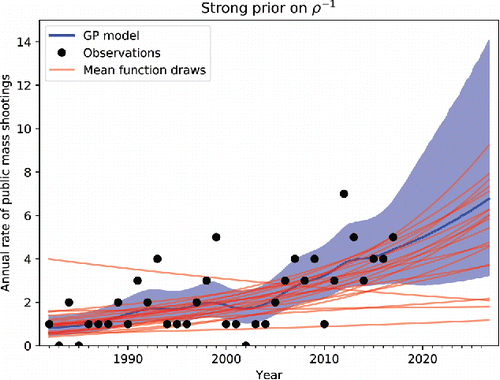
The Gaussian process captures an increase in the mass shooting rate over the decades and some fluctuations against that trend during certain periods. The model does not show any evident deviations from the evolution of the observational time series, although comparison to the data highlights several years with outlying mass shooting totals (e.g., 1993 and 1999). The extrapolated period (> 2017) suggests a range of possible future rates of growth from the 2017 level.

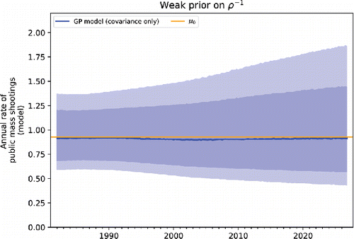
In Figure 1, the comparison between draws of the mean functions (red) and the model posterior (blue) suggests that the mean function captures most of the modeled variation in the shooting rate over time. We can understand the behavior of the Gaussian process covariance function by isolating it from the mean function, as shown in Figure 2. The fact that the interquartile contours never cross the mean (μ₀) indicates that there is never > 75% probability that the annualized trend deviates from the linear mean function. However, there are times when the interquartile range approaches the mean.

Figure 2. Visualization of the observed rate of public mass shootings over time (top) and Gaussian process covariance function for the model with the strong prior on ρ^{− 1} (bottom), isolated by subtracting the mean function from the posterior predictive distribution of the simulated Gaussian process rates (y₂). The shaded regions show the interquartile and [16–84]th percentile ranges.

Next, we visualize the latent Gaussian process under the weak prior for ρ^{− 1} in Figure 3. The figure shows that the Gaussian process does not capture significant short-timescale variations, a direct consequence of loosening the prior to admit longer-timescale covariance functions. This model also generally expresses lower uncertainty in the annual public mass shootings rate. Averaged over the years on which we do prediction, the model with the strong prior has a 5% higher uncertainty in the annualized mass shooting rate than the model with the weak prior. Consistent with the reliance on the parametric, linear mean function, the extrapolated predictions do not account for any substantial probability of decrease in the rate of public mass shootings after 2017. Figure 4 underscores the dominance of the mean function over the covariance function in this model by visualizing the isolated Gaussian process covariance function, which shows virtually no deviation from the mean.

Figure 3. Posterior distribution of the Gaussian process for the annualized mass shooting rate under the weak prior on ρ^{− 1}. Plotted elements are as in Figure 1, except that the random draws (red lines) are omitted for clarity.

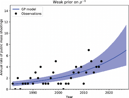
Figure 4. Visualization of the isolated Gaussian process covariance function for the model with the weak prior on ρ^{− 1}, as in Figure 2.

3.3. Posterior Correlations

Because we adopt a fully Bayesian approach, we can interrogate samples from the posterior distribution to understand correlations and dependencies between parameters in our model. We fit a simple linear model to understand relationships between key parameters in the multivariate posterior distribution.

First, we fit a model for ρ^{− 1} as a function of the other major parameters of the model with the strong prior on ρ^{− 1}. Table 1 shows that the most significant correlation is between ρ^{− 1} and η. When we visualize this correlation (Figure 5), we observe that the level of posterior curvature associated with these two variables is small in this model, though significant. The implication is that our choice of prior on ρ^{− 1} implies some constraint on the amplitude of short timescale variations the Gaussian process will recover. The results show that ρ^{− 1} is effectively independent of the intercept for the mean function (μ₀) and only very weakly dependent on the mean function slope (μ_b), as well as the dispersion parameters (σ and ${\mathrm{NB}}_{{\varphi }^{-1}}$). This indicates that our choice of prior will not substantially affect inferences on these parameters or the aspects of the Gaussian process they control.

Figure 5. Visualization of a two-dimensional slice, for η and ρ^{− 1}, of the posterior from the model with the strong prior on ρ^{− 1}. The red shading indicates the density of posterior samples.

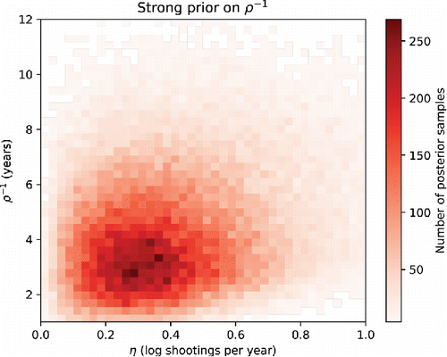
Table 1. Linear model regression coefficients summarizing posterior dependencies in the model with the strong prior on ρ^{− 1}. The predictors have been standardized so the coefficients of the linear model are directly comparable.

Coefficient	Value	Std. error	Sign.
Intercept	0.000	0.003
η	0.243	0.003	^**
μ0	0.032	0.006	^**
μb	0.036	0.006	^**
${\mathrm{NB}}_{{\varphi }^{-}1}$	0.014	0.003	^**
σ	0.014	0.003	^**

However, the above correlation results apply only to the range of ρ^{− 1} values admitted by our strong prior. The relationships between variables may differ in posteriors that have support over larger ranges of ρ^{− 1}, as in our model with the weak prior.

When we explore the same correlation in the posterior of the model with a weak prior on ρ^{− 1}, as shown in Table 2 and Figure 6, we find somewhat different results. Again, η is the parameter most significantly correlated with ρ^{− 1}, but now the 2D posterior visualization shows that this correlation is substantially nonlinear. In particular, for this model, η is constrained to much smaller values when the timescale ρ^{− 1} is small. In other words, in models that permit variations from the mean function on timescales smaller than the observational range (∼ 35 years), the amplitude of those variations is constrained to be very small. As a result, as we have seen, the importance of the covariance function is minimized under this prior regardless of the value of ρ^{− 1}. As in the first model, the ρ^{− 1} has a negligible dependence on the other model parameters.

Figure 6. Same as Figure 5, but for the model with the weak prior on ρ^{− 1}.

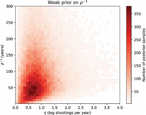
Table 2. Regression coefficients for the model with the weak prior on ρ_{− 1}, as in Table 1.

Coefficient	Value	Std. error	Sign.
Intercept	0.000	0.003
η	0.166	0.003	^**
μ0	0.008	0.004	^**
μb	−0.036	0.004	^**
${\mathrm{NB}}_{{\varphi }^{-}1}$	−0.014	0.003	^**
σ	−0.007	0.003	^**

4. Results

4.1. Parameter Inferences

In Figure 7, we show the marginalized posterior distributions of the parameters of the Gaussian process under the strong prior on ρ^{− 1}. The comparison of the posterior and prior distributions shows strong evidence from the data to identify most hyperparameters. The posterior for μ₀ shows a concentration around a baseline rate of exp ( − 1) ∼ 0.4 to exp (1) ∼ 3 public mass shootings per year at the start of the dataset, 1982, reflecting a variance much smaller than the corresponding prior. The negative binomial overdispersion parameter (φ^{− 1}) is concentrated toward very small values ≪ 1, indicating that the Poisson distribution is a good approximation to the variance in the observations. The amplitude of the Gaussian process covariance function, η, is strongly shifted from the mode of the prior distribution, to a mean of exp (0.5) ∼ 1.6 public mass shootings per year. The variance of the Gaussian process covariance function, σ, has a posterior variance much smaller than the prior distribution.

Figure 7. Sampled posterior distribution for the hyperparameters of the model with the strong prior on ρ^{− 1} (histogram) and corresponding hyperprior distribution (blue line).

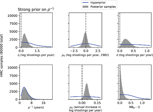
The posterior distribution of ρ^{− 1} is a notable exception. It shows no visual deviation from the prior distribution, indicating that this parameter is not identified by the observations. Therefore, as we have seen, the choice of prior on this parameter will have significant consequences on the posterior.

Next we explore the same marginalized posteriors under the weak prior on ρ^{− 1}, in Figure 8. In this model, most parameters have posterior distributions nearly identical to their distributions under the strong prior on ρ^{− 1}. In particular, the conclusions about the mean function parameters (μ₀ and μ_b), φ, and σ seem robust to the choice of prior. This is consistent with our findings in Section 3.3.

Figure 8. Like Figure 7, but for the model with the weak prior on ρ^{− 1}.

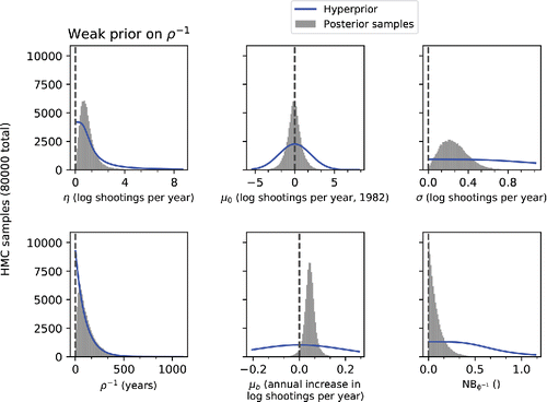
Importantly, the ρ^{− 1} parameter is again largely nonidentified. Its posterior distribution generally follows the weaker prior, although the likelihood suppresses the posterior density for the very smallest values of ρ^{− 1}. The consequence is that the models sampled from the Gaussian process have very long timescales for their covariance function. As we saw in Section 3.3, the weaker prior also has some effect on the amplitude, η, which skews toward larger values than in the first model.

These results validate our decision in Section 3.1 to focus on ρ^{− 1} as a means of understanding the role of prior information in this problem.

4.2. Predictions

We calculate the posterior probability that the annualized rate of public mass shootings has increased in the US since 1982 (μ_b > 0). For the model with the strong prior on ρ^{− 1}, this probability is 98%; for the model with the weak prior, it is 97%. This indicates strong statistical evidence for a long-term increase in the annualized rate of public mass shootings over the past three decades, regardless of our choice of prior for the timescale parameter, ρ^{− 1}.

In linear terms, the mean percentage increase in the rate of public mass shootings is found to be 390 [150, 910]% for the model with the strong prior on ρ^{− 1} and 390 [150, 890]% for the model with the weak prior (quoted ranges are 1σ). While the uncertainty interval is large, the 1σ estimate suggests at least a doubling in the annualized rate of public mass shootings over these three decades, and more likely a quintupling or greater increase. Again, this result is effectively independent of the choice of prior.

For comparison, the U.S. population has grown from ∼ 231 million to 323 million residents (see WorldBank data, http://data.worldbank.org/indicator/SP.POP.TOTL?cid=GPD_1&end=2016&locations=US&start=1982), an increase of 40%, over that same period. The model posterior suggests that the growth rate of public mass shootings has surpassed the rate of population growth with high confidence: 95% for the model with the strong prior on ρ^{− 1} and 95% for the model with the weak prior.

However, any inferences about the response to events or policy interventions within this period may depend on design choices because they will focus on small timescale variations that are sensitive to the prior information provided on ρ^{− 1} (see Section 3.2).

Perhaps the most salient short timescale variation captured by the model with the strong prior on ρ^{− 1} is a dip in the annualized rate of public mass shootings in the years from about 2000 to 2005 (see Figure 2). The model has no features that would seek to explain the causal origin of this dip, but does constrain its size. There is a notable juxtaposition in timing with the Columbine High School massacre (1999), which is understood to have spawned dozens of “copycat” threats and attacks over time (Kostinsky et al. 2001; Simon 2007; Larkin 2009). Apparently this phenomenon did not translate to elevated nationwide incidence of public mass shootings beyond the underlying long-term trend captured by the mean function. Under the model with the weak prior on ρ^{− 1}, there is no short timescale response (Figure 4).

The largest positive deviation from the mean function under the strong prior occurs between about 1988 and 1993 (Figure 2). During that time, the mean function itself is very small (Figure 1), so this does not represent a large absolute deviation.

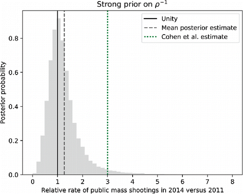
Figure 2 does also show a small elevation from the mean function between about 2011 and 2014. Cohen et al. (2014) reported a tripling in the rate of mass shootings during this same time frame on the basis of an SPC methodology. While we have reported that the increase in the rate of public mass shootings over the past three decades is likely to be a factor of several, we find much less evidence for such a dramatic increase over this 4 year period. Our model with the strong prior on ρ^{− 1} predicts better than even odds (60%) that there was an increase during that time, but the probability that it was as high as a tripling is small (3%). The mean of the posterior predictive distribution for the 3 year increase in the annualized mass shooting rate under this model is 27% (see Figure 9).

Figure 9. Comparison of estimates for the relative annualized rate of mass shootings between 2014 and 2011. The shaded distribution shows the posterior from our model with the strong prior on ρ^{− 1}. The dotted line shows the result of Cohen et al. (2014).

As noted in Section 3.2, there is also a tradeoff between the sensitivity to identifying short timescale variation in the evolution of the mass shooting rate and the level of uncertainty in the year-to-year estimate of the annualized mass shooting rate, controlled by the expression of prior information on the timescale parameter. In this case, the impact of the prior choice on the uncertainty is small (5% as quoted in Section 3.2) and manifests as only minor difference between the probabilities we report for the two models in this section.

These findings illustrate that, for analysis of timeseries data in low-frequency event domains like mass shootings, it is critical to a policy analyst’s role to carefully and consciously assert prior information about the relevant timescale for interventions to have an effect to support policymaking through assessment of available data. As we have shown, failing to assert significant prior information about the timescale parameter can lead inevitably to the conclusion that short timescale variation does not occur. In a policymaking context, this is a recipe for inaction.

4.3. Comparison to SPC Methodology

The comparison between the SPC and Gaussian process methodologies is an interesting contrast in approach to timeseries modeling of rare events. In this context, the SPC methodology can be viewed as a sequence of hypothesis tests for a change in the frequency of an event type (see Woodall 2018 for a discussion). Adopting a common heuristic, Cohen et al. interpret nine or more sequential occurrences where the time between events is lower than the previous running average of time between events as evidence for a significant shift in the underlying frequency.

The most fundamental difference between the approaches is the quantity targeted for analysis: time between events versus annualized rate. While the Gaussian process methodology requires some timescale for binning of the raw data, the SPC methodology has sensitivity to frequencies on any timescale because it directly analyzes the time between events. However, the choice of significance threshold (how the running average is constructed and the threshold of number of deviant events in sequence) effectively expressed prior information about the timescale for change in the measured rate.

Another contrast is between the hypothesis testing framework of SPC and the generative modeling framework of the Gaussian process. The generative model supports hypothesis testing of posterior quantities, while also providing a continuous model of the underlying evolution of the test quantity. A fundamental benefit of the generative model is the opportunity to assess uncertainty of test statistics from the fully Bayesian posterior distribution, as well as the opportunity to perform inference on model parameters (see Section 4.2). The generative model can also be used for additional tasks such as interpolation, to predict the probability distribution of rates at any arbitrary time, and extrapolation, to predict the probability distribution of rates outside of the observed time range.

A more subtle distinction between the two approaches is the data effectively included in hypothesis tests for changes in frequency. SPC implies a sequential approach, where each contiguous segment of observations is compared only to some average across observations directly preceding it. The Gaussian process model fit is constrained by all observations simultaneously, so that the estimate of the underlying event rate is influenced by the nearest observed annualized rate as well as all observations before and after.

This discussion contrasts two of a myriad of approaches to extract insight from timeseries data. More generally, we advocate for the use of generative models, which explicitly specify all elements of model design including prior information as in Section 3.1. Further, we recommend the use of fully Bayesian inference, so that the consequences of choices about prior distributions including parameter correlations can be straightforwardly explored as in Section 3.3. The model we define in Section 3 has the added benefit of combining parametric and nonparametric components, to allow for direct inference on salient model parameters as well as the capture of subtle nonlinearities in empirical data as in Section 4.2.

5. Conclusion

We have designed and implemented a negative binomial regression model for the annualized rate of public mass shootings in the United States based on a Gaussian process with a time-varying mean function. This design yields a predictive model with the full nonparametric flexibility of a Gaussian process to explain short timescale variation, while retaining the clear interpretability of a parametric model by isolating and jointly modeling long-term (timescale of decades) evolution in the shooting rate. We have applied this model to a commonly cited historical dataset of U.S. public mass shootings and explored the implications of explicit choices about the prior information provided on the timescale parameter for the Gaussian process covariance function in this model. Our primary conclusions are as follows:

• We use posterior simulations and predictive checks to demonstrate the efficacy of the Gaussian process model in generating and fitting the observations of the annual mass shooting rate from the Mother Jones database.

• With a 98% probability, we find that the annualized rate of public mass shootings has risen over the past three decade. The posterior mean estimate for the increase in the public mass shooting rate since 1982 (390 [150, 910]%) suggests at least a doubling, and more likely a quintupling, of the annualized rate over that time.

• We explore the effects of prior choices on the posterior and visualize posterior curvature between hyperparameters. We demonstrate that the choice of prior has negligible impact on inferences about the long timescale variation of mass shooting events, but significant impact on inferences about short timescale variations that may be relevant to evaluating policy interventions.

• We contrast our generative modeling approach using fully Bayesian inference to the statistical process control (SPC) methodology, and discuss wider implications for choices in model design for policy analysis of timeseries data.

As future work, we would like to expand the model for public mass shootings presented here to address causal relationships with policy-relevant factors. In particular, the Gaussian process can be expanded to incorporate additional predictors such as data from multiple countries or indicators of policy changes like firearm sales rates. A multi-output Gaussian process could also model covariant outcomes like number of fatalities or type of weapon used. Combined with a review of the choices in data collection and a careful analysis of the role of prior information in determining the model posterior, this work can lead to policy recommendations to help control the occurrence of these events in the future.

Supplementary Materials

MCMC Simulation: Additional description and diagnostics related to the Markov chain Monte Carlo simulations used to make inferences under the model described in Section 3 (PDF).

Data and Code: All data and code associated with this project has been posted to a git repository located at https://github.com/nesanders/spp-massshootings (Repository).

Acknowledgments

The authors gratefully acknowledge Michael Betancourt, Amy Cohen, Deb Azrael, and Matt Miller for their insightful feedback on versions of this manuscript and the statistical techniques applied, the organizers and attendees of StanCon 2017 for providing feedback on a draft version of this work, and the two anonymous reviewers for their feedback.

References

- Blair, J. P., and Schweit, K. W. (2013), “A Study of Active Shooter Incidents in the United States Between 2000 and 2013,” Texas State University and Federal Bureau of Investigation, U.S. Department of Justice.
- Cohen, A. P., Azrael, D., and Miller, M. (2014, October 15), “Rate of Mass Shootings has Tripled Since 2011, Harvard Research Shows,” Mother Jones. Available at https://www.motherjones.com/politics/2014/10/mass-shootings-increasing-harvard-research/.
- Follman, M. (2014, October 21), “Yes, Mass Shootings are Occurring More Often,” Mother Jones. Available at https://www.motherjones.com/politics/2014/10/mass-shootings-rising-harvard/.
- Fox, J. A., and Levin, J. (2015), “Mass Confusion Concerning Mass Murder,” The Criminologist, 40, 8–11.
- Gelman, A., Jakulin, A., Grazia Pittau, M., and Su, Y.-S. (2009), “A Weakly Informative Default Prior Distribution for Logistic and Other Regression Models,” The Annals of Applied Statistics, 2, 1360–1383.
- Heaton, M. J. (2014), “Wombling Analysis of Childhood Tumor Rates in Florida,” Statistics and Public Policy, 1, 60–67.
- Kostinsky, S., Bixler, E., and Kettl, P. (2001), “Threats of School Violence in Pennsylvania After Media Coverage of the Columbine High School Massacre: Examining the Role of Imitation,” Archives of Pediatrics & Adolescent Medicine, 155, 994–1001.
- Larkin, R. W. (2009), “The Columbine Legacy: Rampage Shootings as Political Acts,” American Behavioral Scientist, 52, 1309–1326.
- Lott, J. R. (2014, October 6), “The FBI’s Misrepresentation of the Change in Mass Public Shootings,” Academy of Criminal Justice Sciences Today, March 2015. DOI: http://dx.doi.org/10.2139/ssrn.2524731
- Rasmussen, C. E., and Williams, C. K. I. (2005), Gaussian Processes for Machine Learning, Cambridge, MA: The MIT Press.
- Roberts, S., Osborne, M., Ebden, M., Reece, S., Gibson, N., and Aigrain, S. (2013), “Gaussian Processes for Time-Series Modelling,” Philosophical Transactions of the Royal Society A, 371, 20110550.
- Rothe, C. (2010), “Nonparametric Estimation of Distributional Policy Effects,” Journal of Econometrics, 155, 56–70.
- Simon, A. (2007), “Application of Fad Theory to Copycat Crimes: Quantitative Data Following the Columbine Massacre,” Psychological Reports, 100, 1233–1244.
- Sun, A. Y., Wang, D., and Xu, X. (2014), “Monthly Streamflow Forecasting Using Gaussian Process Regression,” Journal of Hydrology, 511, 72–81.
- Woodall, W. H. (2018), Controversies and Contradictions in Statistical Process Control, Journal of Quality Technology, 32(4), 341–350, DOI: 10.1080/00224065.2000.11980013.