On Racial Disparities in Recent Fatal Police Shootings

Abstract

Fatal police shootings in the United States continue to be a polarizing social and political issue. Clear disagreement between racial proportions of victims and nationwide racial demographics together with graphic video footage has created fertile ground for controversy. However, simple population level summary statistics fail to take into account fundamental local characteristics such as county-level racial demography, local arrest demography, and law enforcement density. Using data on fatal police shootings between January 2015 and July 2016, I implement a number of straightforward resampling procedures designed to carefully examine how unlikely the victim totals from each race are with respect to these local population characteristics if no racial bias were present in the decision to shoot by police. I present several approaches considering the shooting locations both as fixed and also as a random sample. In both cases, I find overwhelming evidence of a racial disparity in shooting victims with respect to local population demographics but substantially less disparity after accounting for local arrest demographics. I conclude the analyses by examining the effect of police-worn body cameras and find no evidence that the presence of such cameras impacts the racial distribution of victims. Supplementary materials for this article are available online.

KEYWORDS:

• Bootstrap/resampling
• Police shootings
• Racial bias

1 Introduction

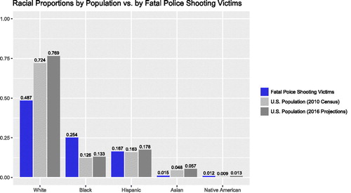
The extensive media coverage of fatal police shootings in recent years in the United States has fueled political debate and sparked widespread controversy. Due in part to this increased attention as well as concerns regarding federal data collection methods (Kobler (1975), Fyfe (2002), Klinger (2012), Nix et al. (2017), Klinger and Slocum (2017), Williams, Bowman, and Jung (2019), Cesario, Johnson, and Terrill (2019), Klinger et al. (2016), and White (2016)), The Washington Post began compiling data on each fatal police shooting taking place in the United States beginning in 2015 (Washington Post 2016). By raw totals, White victims far outweigh all other racial groups, accounting for nearly half (733) of the 1505 documented shootings between January 1, 2015 and July 11, 2016.¹ However, when we compare the proportions of fatal shootings to the population demographics in the United States (United States Census Bureau 2016), we see that the proportion of fatal shootings of Blacks is substantially higher than the population proportion, whereas the proportions of White and Asian fatal shooting victims fall below their respective population proportions; see Figure 1.

Fig. 1 Racial proportions by total US population vs. by fatal shooting victims. Fatal shooting proportions were tabulated directly from the data provided by The Washington Post (2016) dataset; population proportions are shown according to the United States Census Bureau (2016).

If key population characteristics such as racial demography and law enforcement density could be assumed to be relatively uniform throughout the United States, this information alone could be considered sufficient to reasonably conclude that the racial proportions (and totals) of fatal police shootings are different from what would be expected under the assumption that race is independent of an officers decision to take potentially lethal action with a firearm. This assumption, however, is simply not reasonable for a large, diverse area like the United States. Thus, given the number of fatal police shootings that occurred between January 1, 2015 and July 11, 2016, the key questions I seek to address in the remainder of this article are: Taking into account local characteristics, how many individuals from each race would be reasonable to expect if the fatal shooting victims could be seen as a random sample from the localized population and are the observed victim totals in line with such expectations.

In attempting to answer these, I make use of the fatal police shootings dataset compiled by the Washington Post as well as datasets containing county-level racial demography, law enforcement density, and local arrest demography. Importantly, I stress that I examine the database of fatal police shootings in totality. In particular, I make no attempt to segment these shootings into those which might be considered “justified” or “nonjustified” and I do not consider whether or with what the victim may have been armed at the time of the shooting. Though the dataset from the Washington Post does contain some information of this sort, it is difficult to determine in many instances whether a suspect “armed” with, for example, a cell phone or a tape measure, actually attempted to present these items as weapons or whether they simply happened to be in their possession at the time of the incident.

Studies related to police shootings and the use of force have long produced a tremendous amount of literature; for a small sample of research from the past two decades, see, for example, Adams et al. (1999), Alpert and Dunham (2004), Alpert and Dunham (1997), Ariel, Farrar, and Sutherland (2015), Fridell and Lim (2016), Legewie and Fagan (2016), Smith (2014), Lim, Fridell, and Lee (2014), Paoline and Terrill (2007), Kop and Euwema (2001), Ridgeway (2016), and Fryer (2016). As already eluded to, however, reliable data on this topic has proven extremely difficult to obtain with numerous studies continually finding underreporting in federal databases by as much as 50% (Kobler 1975; Fyfe 2002; Klinger 2012; Nix et al. 2017; Klinger and Slocum 2017; Williams, Bowman, and Jung 2019; Cesario, Johnson, and Terrill 2019; Klinger et al. 2016; White 2016). Indeed, in line with this already well-established finding, the data from the Washington Post used here contains information on 515 fatal police shootings through July of 2016, whereas the FBI’s Supplemental Homicide Report (United States Federal Bureau of Investigation 2019) contains only 439 incidents for the entire year. As remarked by Fyfe (2002) and later recalled by Klinger and Slocum (2017), it remains the case that “the best data on police use of force come to us not from the government or from scholars, but from the Washington Post.” In light of this, researchers have recently begun focusing on more complete data provided by large journalistic outlets. As one example, Nix et al. (2017) utilized the Washington Post data from 2015 to investigate incidents they determined to be “threat-perception failures” and concluded that certain minority groups were less likely to be attacking an officer and/or armed at the time of the shooting. Klinger and Slocum (2017) take issue with this study, however, for reasons much in line with those noted in the preceding paragraph. The authors argue that even unarmed individuals can pose a potentially serious threat and point to at least four separate incidents in which officers were attacked with objects that might be otherwise innocuous (e.g., metal pole, tree branch) and yet victims were categorized as “unarmed” in the data provided by the Washington Post. I emphasize that the work referenced above merely scratches the surface of all research on police-involved shootings. For a more thorough accounting of existing research in this area, the interested reader is referred to the literature reviews provided in Ridgeway (2016) and Nix et al. (2017) as excellent potential starting places.

Perhaps, the study most similar in spirit to the work presented here was published very recently by Cesario, Johnson, and Terrill (2019). Here too the authors point out the potential issues with seeking to identify bias by comparing the racial proportions of police shooting victims to nationwide racial demographics. The authors instead argue that police are more likely to use deadly force in crime-related interactions and therefore utilize federal crime data to estimate national rates of criminal involvement for both Blacks and Whites. Using police shooting data collected by The Guardian, they then compute the odds of both races being shot, ultimately concluding that no racial disparity exists relative to the estimated rates of criminal involvement.

As noted above, the work here pushes beyond simple comparisons of nationwide proportions. Instead, using the data collected by the Washington Post, I focus on local characteristics of the populations where police shootings actually took place in 2015 and 2016. Furthermore, I use a resampling approach that allows us to estimate the entire distribution of the number of expected victims from each race under various setups rather than obtaining only a single number summary. This approach thus allows us to more fully characterize the likelihood of observing the various counts actually observed during those years.

The remainder of this article is laid out as follows. A brief overview of the datasets is provided in Section 2 with a more thorough description and accounting given in the Appendix. Section 3 employs a resampling scheme to estimate the distributions of total fatal police shooting victims by race, conditional on the locations where the observed shootings took place. Section 4 considers an alternative scheme wherein the locations are selected at random and weighted according to the relative law enforcement density and Section 5 incorporates local arrest demography into the analysis. Section 6 compares the racial proportions of police shooting victims in incidents where the responding officers were wearing body cameras to those in which no body camera was present. Finally, Section 7 concludes with a careful discussion of these results. In addition to the details provided in the Appendix, an accompanying R file is also provided to reproduce all results and calculations.

2 Data Overview

The analyses in the following sections make use of a total of five different publicly accessible datasets. Here, I provide a short overview of each. Appendix B contains more detailed information including access instructions as well as a thorough accounting of modifications and corrections made to the original data in order to perform the analyses. The abbreviations and numeric citations listed indicate how each individual dataset will be referenced in future sections.

• (WP) Washington Post (2016): The primary dataset of interest here, containing information on recent fatal police shootings as collected and reported by the Washington Post. Note that this dataset contains only instances of fatal shootings; nonfatal shootings and other police encounters resulting in death are not included. In addition to the date, city, and state of these fatal shootings, the dataset also contains a number of other features such as what (if anything) the victim was armed with, an indicator for whether the responding law enforcement officers were wearing body cameras, an indicator for whether the victim displayed signs of mental illness, the victim’s (estimated) threat level, in what fashion (if at all) the victim was fleeing, as well as age, gender, and race of the victim.² Based on the city and state information, county information was later imputed according to information provided by the National Association of Counties (NACo) National Association of Counties (2016).

• (DEM) United States Census Bureau (2016): This dataset contains information on county-level racial demographics in the United States based on the 2010 U.S. Census. Information is provided for a total of 3142 counties or parishes. For each county or parish, the total population is provided along with the total population of a particular race. The races included are: White (W), Black (B), Native American and/or Alaskan Native (NA), Asian (A), Native Hawaiian and Other Pacific Islander (NH), and finally “Two or More” (T). While it’s generally easier to refer to this dataset as a single object, in each of the resampling analyses, I make explicit use of two separate datasets containing this demographic information: one based on the 2010 census data itself and another based on the projected demographics in 2016.

• (LEE) Federal Bureau of Investigation (2016): This dataset contains information on county-level Law Enforcement Employment collected by the FBI through the 2011 Uniform Crime Reporting (UCR) Program. Information is provided for a total of 2797 counties or parishes. For each county or parish, the total number of law enforcement employees is provided and broken down by officers and civilians. From the FBI data disclosure, “the UCR Program defines law enforcement officers as individuals who ordinarily carry a firearm and a badge, have full arrest powers, and are paid from governmental funds set aside specifically to pay sworn law enforcement” whereas “civilian employees include full-time agency personnel such as clerks, radio dispatchers, meter attendants, stenographers, jailers, correctional officers, and mechanics”.

• (ARREST) United States Department of Justice (2017): This dataset contains information on local, county-level arrests by age, sex, and race in 2013. For each reporting county, a number of different offenses are reported and for each offense type, the total number of arrests made according to age, sex, and race demographics is provided. In total, 2754 counties report at least one crime. The races included in this dataset are White (W), Black (B), Native American and/or Alaskan Native (NA), and Asian (A). County information is provided by FBI UCR numeric code instead of name.

• (CODES) ICPSR (1999): This dataset contains state, county, and parish names along with Uniform Crime Reports (UCR) and Federal Information Processing Standards (FIPS) numeric codes. The primary purpose of this dataset is to facilitate linking between the ARREST data which contains only UCR county codes and the WP, DEM, and LEE datasets which contain only the county or parish names.

3 Local Population Demographics

We now begin the resampling analyses to investigate how unlikely the observed racial distributions of fatal police shooting victims between January 2015 and July 2016 would be if the victims of these shootings could be considered a random sample from the local population in which the shootings took place and no racial biases were present. As discussed above, it can be readily seen from Figure 1 that the racial proportions of victims appear out-of-line with the nationwide racial demographics; here I use the WP and DEM datasets to determine whether the same can be said after taking into account the local racial demographics.

Of the 1505 fatal shootings in the WP dataset, only one shooting location did not appear in the DEM dataset; this was WP ID number 686 which occurred in Las Cruces, NM in Doña Ana County. Furthermore, there are a total of 77 additional victims in the WP dataset for which race information is missing. After removing these, there are a total of 1427 victims for which both the race of the victim and the county-level racial demographics are known. Of these, 733 (51.4%) were White, 382 (26.8%) were Black, 251 (17.6%) were Hispanic, 18 (1.3%) were Native-American, 22 (1.5%) were Asian, and 21 (1.5%) are listed as “Other.”

To investigate the plausibility of this observed racial distribution, I performed 1000 simulations in which an individual race was selected at random from each shooting location according to the racial proportions in the county in which the shooting occurred. That is, if a particular shooting occurred in a county in which the proportions were 50% White, 20% Black, 5% Native American, and 5% Asian, then W, B, N, or A would be selected with probabilities 0.5, 0.2, 0.05, and 0.05, respectively. The total number of victims from each race were then summed and the entire process repeated 1000 times. Thus, for each race, we obtain an estimated distribution of victim totals under the assumption that fatal shooting victims can be considered a random sample from the racial demographics of the county in which the shooting occurred.

Before undertaking these simulations, we first need to address the disagreement in racial categories between the WP and DEM datasets: the WP dataset contains the racial categories W, B, NA, A, H, and O while the DEM datasets contain the categories W, B, NA, A, NH, and T. Beyond these racial categories, the DEM datasets also contain information on how many residents of each race are Hispanic. Given this additional information, accounting for the Hispanic (H) population in our resampling procedure is straightforward: once a race is selected, we either keep that race or replace it by “Hispanic” with probability weighted according to the local Hispanic population. More formally, let H_ij denote the proportion of race i that is Hispanic in county j. Supposing that race i is that which is first randomly selected, we record a victim belonging to that race with probability $1-H_{ij}$ and instead record a race of “Hispanic” with probability H_ij.

We now finally need to determine whether the O classification in the WP dataset roughly corresponds to the combined NH and T classifications in the DEM datasets. Looking at these datasets, we see that the average proportion of the population classified as either NH or T is approximately 2.48% according to the 2010 census and 2.86% according to the 2016 projections. According to the U.S. Census Bureau (2016) Quickfacts, W, B, NA, and A made up approximately 76.9%, 13.3%, 1.3%, and 5.7% of the population, respectively, leaving 2.8% of the population for an “Other” category. Since this is in close agreement with the raw averages from the DEM datasets, we proceed accordingly treating NH and T in the DEM datasets as the equivalent of the O classification in the WP dataset. That is, whenever either NH or T is selected in the resampling procedure, we first randomly determine whether to count the observation as Hispanic and if not, we count the observation as Other (O).

Figure 2 shows the total number of police shooting victims by race for each of the six classifications given in the WP dataset along with the expected totals with respect to both the 2010 census data and the 2016 projections. These expected totals for each race were computed by simply taking the mean of the 1000 resampled victim counts and rounding to the nearest integer. Here we see the same general pattern as in Figure 1: while the total number of Native-American victims seems to be in line with what would be expected, the observed totals are fewer than expected for Whites and Asians while much greater than expected for Blacks. In fact, according to these results, more than twice as many Blacks were fatally shot by police than would be expected if the shooting victims could be considered a random sample from the local population. Note that Figure 2 describes only how the true victim totals compare to the mean of the observed empirical distribution; density estimates for total victims of each race are shown in Figure 3 in Section 4.

Fig. 2 Fatal police shooting victim totals vs. expected totals by local racial demographics assuming a fixed shooting location.

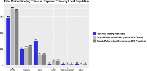
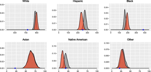
Fig. 3 Kernel density estimates for victim totals by race assuming fixed shooting locations (gray) or random locations (red) with respect to the 2010 census data on local racial demographics. Blue points along each horizontal axis correspond to the observed victim totals in the WP dataset.

In order to formalize these results, we can obtain p-value estimates to assess whether the observed victim totals are significantly different from what would be expected by comparing the observed total to the totals found in our resampling procedure and counting the number of resampled totals that were more extreme than that observed. The probability of observing a victim total more extreme than that observed is calculated as follows:$${\widehat{p}}_r=2\times \frac{\min \{\#\text{greater}\text{than}{T}_r,\#\text{less}\text{than}{T}_r\}}{N},$$where T_r denotes the observed victim total for race r so that $\#$ greater (or less) than T_r counts the number of estimates of victim totals out of the N = 1000 that resulted in a victim count more (or less) than the observed total. These estimates take the form of binomial random variables and thus have standard deviation $\sqrt{p_r(1-p_r)/N}$. We don’t know the true (exact) p-value p_r but the standard deviation is bounded above by $\frac{1}{2\sqrt{N}}\approx 0.015$. For a further discussion on these errors the reader is referred to Efron and Tibshirani (1994); Good (2005); Ojala and Garriga (2010).

A table of such p-values is shown in Table 1. Note that p-values are all 0 for Whites, Blacks, and Asians with respect to both the 2010 census and 2016 projected racial demographics indicating that the observed victim totals are significantly different from what would be expected. On the other hand, we see highly nonsignificant results for Native Americans while for Hispanics and Other, we see significant results at an α-level of 0.05 based on the 2016 projected racial demographics, but not according to the 2010 census. Results remaining significant after a Bonferroni correction are shown in bold.

Table 1 P-values based on the empirical distribution of victim totals from each race based on the 2010 census data and 2016 projections.

	Fixed locations		Random locations
	2010 Census	2016 Proj.	2010 Census	2016 Proj.
White	0	0	0	0
Hispanic	0.078	0.002	0.333	0.836
Black	0	0	0	0
Asian	0	0	0	0
Native Am.	0.97	0.984	0.018	0.024
Other	0.102	0.02	0.239	0.056

NOTE: Results remaining significant after a Bonferroni correction are shown in bold.

Remark: The p-value formula above of the form m/N represents the standard unbiased estimate where N denotes the total number of resamples and m denotes the number of resulting statistics more extreme than that originally observed. In permutation/randomization-test settings, some (see, e.g., Phipson and Smyth 2010) have instead advocated for a biased estimate of the form $(m+1)/(N+1)$ that accounts for the original statistic in order to ensure that the estimated p-value does not inflate the Type I error rate of the resulting test. All tests performed in this article involves a large number of resamples ($N\ge 1000$) and thus the two estimates are nearly equivalent, but nonetheless, estimates of the latter form can be easily calculated from the tables of p-values given throughout the remainder of this article.

4 Treating the Shooting Locations as Random

The preceding analysis suggests strongly that the racial proportions of fatal police shooting victims are not representative of the racial demography of the counties in which those shootings occurred. It may be reasonable, however, to consider that there is some randomness involved with the shooting locations themselves. For example, if police are led on a high-speed chase across counties that ends with the suspect dead after a shootout, this would count as a fatal police shooting that occurred in that final county and would ignore information about the county in which the incident originated. As another example, it is entirely possible that around the same time when some of these incidents occurred, other unrelated nonfatal shootings occurred under similar circumstances elsewhere in the United States. Since the WP dataset contains only information on fatal police shootings, these other possible incidents remain unaccounted for in the previous analysis.

Thus, let’s now consider a setup whereby the locations of the 1427 shootings are taken as a random sample from all U.S. counties, weighted by law enforcement officer employment. That is, instead of choosing a race according to the local racial demographics of the counties in which these shootings actually occurred, we instead select counties at random with those employing a larger number of law enforcement officers being more likely to be selected.

In order to perform this kind of resampling, we make use of the LEE dataset described in Section 2 that contains law enforcement employment totals for both officers and civilians. In this procedure, we resample according to the law enforcement officer employment as these individuals are specifically defined as those who “ordinarily carry a firearm and a badge” (Federal Bureau of Investigation 2016). Note that while we could instead weight the resampling by total law enforcement employment, we do not expect that this alternative approach would produce significantly different results as the correlation between officer employment and total employment is exceptionally high at 0.97.

The remainder of the resampling procedure is identical to that laid out in Section 3, except that this time we employ a total of 2000 simulations—double the previous number—in order to account for the additional randomness involved in selecting a location. The same reasoning as the previous section gives that the standard deviation of the resulting p-value estimates should be bounded above by $\frac{1}{2\sqrt{2000}}\approx 0.011$. The empirical densities of victim totals by race with respect to the 2010 census data are shown in Figure 3. The densities with respect to the 2016 projections are extremely similar and the corresponding plots are thus reserved for Appendix C. Note that for the Asian and Other races, the densities of victim totals based on fixed locations are nearly identical to those where locations were selected at random. For the White and Black races, the densities based on random locations appear shifted slightly right (higher expected totals), while for the Hispanic and Native American races, the densities based on random locations are shifted more substantially left (lower expected totals).

Though the densities appear to shift a bit for some races when considering the shooting locations as random, overall the same general patterns appear to be presented: for the Hispanic, Native-American, and Other races, the observed victim totals (blue points in Figure 3) appear more reasonable based on the empirical distributions while for the White, Black, and Asian races, the observed totals lie far from the densities estimated via the resampling procedures. To examine this more formally, we can compute p-values in the same fashion as described in Section 3 with respect to these new densities based on random shooting locations. A table of these p-values along with those calculated assuming a fixed shooting location is shown in Table 1.

Looking at Table 1, it is immediately clear that taking into account local population demographics does not help explain the victim totals observed for Whites, Blacks, and Asians. Assuming a level of $\alpha =0.05$, for Hispanics and Others, we would reject the null hypothesis that the observed victim totals could have come from the distributions based on the 2016 projections with fixed shooting locations, while we fail to reject in every other case. For Native-Americans, we fail to reject the null hypothesis for the densities based on fixed shooting locations, but would reject it according to the densities estimated assuming random shooting locations.

5 Local Arrest Demographics

In the previous analyses, we investigated how many victims from each race might be expected if the victims were thought of as a random sample from the local population. For some races—White, Black, and Asian, in particular—the expected victim totals were far from what was observed in the WP dataset, suggesting that this assumption is a bit too naïve and unreasonable. In very recent work, Cesario, Johnson, and Terrill (2019) make a similar point, arguing that disparities in police shooting rates across race should be investigated relative to rates of criminal involvement. The authors attempt to estimate nationwide crime rates for both Blacks and Whites, focusing in particular on murder/nonnegligent manslaughter, violent crime, and weapons violations. Such crimes, they claim “are the most aggressive in terms of interpersonal violence and, as such, are appropriate proxies for exposure to those situations during which police may be more likely to use deadly force” (Cesario, Johnson, and Terrill 2019). The authors ultimately find no evidence of anti-Black disparities relative to their estimated crime rates.

Here, rather than estimate a single nationwide rate of criminal involvement for each race, we make use of the ARREST data described in Section 2 which contains information on local, county-level arrests by offense, age, sex, and race. Since county information is provided only by FBI UCR numeric codes, the CODES dataset was also used to impute county names to allow for cross-reference with the datasets used in the previous analyses. The objective here is to employ the same sort of resampling scheme used in the previous analyses except that instead of sampling victim races by weighting with respect to local population demographics, here we weight samples according to local arrest demographics.

Complicating matters is the fact that the ARREST dataset consists of only four racial categories: W, B, NA, and A. If we were to sample from only these races, we would necessarily overestimate the victim totals for each race and thus we need to be sure to account for the additional racial categories—Hispanic (H) and Other (O)—appearing in the WP dataset. Though somewhat unsatisfying, the most reasonable way to accommodate this given the data is to make the assumption that the proportion of arrests in each county of individuals belonging to these additional races are the same as the population proportions. Thus, under this setup, we expect the distributions for H and O to be similar to what was seen in the previous analyses. Fortunately, however, as seen in those previous analyses, the Hispanic and Other races were two in which the number of observed victims seemed to be reasonable with respect to local population demographics. For these reasons, we focus our attention here more heavily on those races—W, B, NA, and A—for which we have the arrest data.

It’s also worth pointing out that to employ this sort of resampling procedure, we need for every location in the WP dataset to contain information in the ARREST dataset and also, because we need to impute information from the DEM dataset into the arrest dataset (to account for the H and O populations), we need entries in the ARREST dataset to have information in the DEM dataset. Because of the disagreement in county information across these three datasets, we need to further subset the WP data to include a total of only 1249 fatal police shooting victims (W (654), B (314), NA (12), A (21), H (229), and O (19)). Further details are provided in the Appendix and the accompanying R file.

We also need to consider how the population of arrestees should be sampled. Given the breakdown by race for each type of offense, we could consider some sort of weighted approach whereby, for example, violent offenses have a higher chance of being selected in a similar spirit to Cesario, Johnson, and Terrill (2019). Indeed, we could potentially assume that individuals previously arrested for violent crimes would be more likely to present a substantial threat to police officers and/or that officers may be more likely to perceive a threat from such known individuals. However, this approach would necessarily involve not only making this additional assumption, but would also require a subjective judgment with regard to what crimes should be considered and how those crimes should be weighted. The decision by Cesario et al. (2019) to focus on “murder/nonnegligent manslaughter, violent crime, and weapons violations” appears to be largely based on personal belief rather than being grounded in hard evidence. There have certainly been numerous highly visible instances in recent years in which fatal police shootings have occurred following what began as relatively routine encounters. While in theory such assumptions could be checked against a national database like the FBI’s Supplemental Homicide Report (2019), as discussed in the introduction, such records are notoriously incomplete and likely suffer from bias as a result of voluntary self-reporting. Given the lack of strong empirical evidence suggesting that all or even the vast majority of police shooting victims are violent criminals, we elect to not make such assumptions and instead aggregate arrest totals across offense types creating a single row of data for each county corresponding to the total number of arrests per race in that county.

As in the previous analyses, we consider resampling procedures based on the fixed locations in which the observed shootings took place and also consider the randomized approach whereby counties are selected according to police employment totals. Because information needs to be imputed for the H and O populations, each procedure was also run twice: once using the 2010 census data to perform the imputation and once using the 2016 demographic projections. The resulting density estimates calculated with respect to the 2010 census data are shown in Figure 4; the densities calculated using the 2016 projections are very similar and thus are reserved for Appendix C.

Fig. 4 Kernel density estimates for victim totals by race assuming fixed shooting locations (gray) or random locations (red). Blue points along each horizontal axis correspond to the true (observed) victim totals from that race in the WP dataset. Victim races selected according to local arrest demographics with races missing arrest totals (Hispanic and Other) sampled according to the 2010 census data.

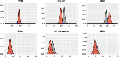
It is immediately clear based on a quick visual inspection that the observed victim totals appear much more reasonable with respect to these distributions than with respect to those based only on local population demographics as investigated in Sections 3 and 4. To be thorough, we compute p-values in the same fashion as in those previous sections with respect to these new densities. A table of these p-values is shown in Table 2. Note that Hispanic and Black are the only races for which a significant result is found at the $\alpha =0.05$ level and even for these races, the estimated totals are significant with respect to only two distributions and not significant with respect to the other two. No results remain significant after a Bonferroni correction.

Table 2 P-values based on the empirical distribution of victim totals from each race based on the 2010 census data and 2016 projections.

	Fixed locations		Random locations
	2010 Census	2016 Proj.	2010 Census	2016 Proj.
White	0.266	0.936	0.333	0.925
Hispanic	0.540	0.046	0.003	0.116
Black	0.004	0.008	0.229	0.287
Asian	0.220	0.198	0.209	0.212
Native Am.	0.412	0.478	0.509	0.409
Other	0.186	0.064	0.334	0.116

NOTES: No results remain significant after a Bonferroni correction.

Furthermore, examining these p-values alone can be somewhat misleading. For both the Black and Hispanic races, we can see visually from the densities in Figure 4 (also see Figure 6 in the onlines appendices) that the observed victim totals seem to lie “in between” the densities based on fixed vs. random locations. Thus, while the observed Hispanic victim total is somewhat higher than might be expected if the locations are assumed to be random, it is somewhat lower than what would be expected if the locations are seen as fixed. For Black victims on the other hand, the opposite is true: the number of victims observed is on the very high end of what would be expected assuming fixed locations, but on the low end of what would be expected if the shooting locations are seen as random. In the way of final confirmation that these distributions are more appropriate, Table 4 in the Appendix shows the number of standard deviations the observed totals lie from the expected totals with respect to each distribution estimated in these and previous analyses. For Whites, Asians, and Blacks, the observed totals fall at least 6, 5, and 14 standard deviations from the expected totals when the resampling is done with respect to local population demographics. When the resampling is done instead with respect to local arrest demographics, the observed totals lie mostly within 1 to 2 standard deviations of what would be expected.

6 Body Camera Effects

Finally, yet another interesting feature of the WP dataset is an indicator variable for whether the officers involved were wearing body cameras. Recall that of the 1505 total fatal shootings recorded in the WP dataset, 1428 contain the (known) race of the victim. Among these instances, the officers involved were wearing body cameras 132 times and thus no body cameras were present in the majority (1296) of instances. The breakdown by race and body camera is shown in Table 3 as a standard ${\chi }^2$ contingency table.

Table 3 Race vs. Body Camera ${\chi }^2$ contingency table.

	W	B	NA	A	H	O	Total
BodCam	64 (67.8)	38 (35.3)	4 (1.7)	1 (2.0)	24 (23.3)	1 (1.9)	132
No BodCam	669 (665.2)	344 (346.7)	14 (16.3)	21 (20.0)	228 (228.7)	20 (19.1)	1296
Total	733	382	18	22	252	21	1428

NOTES: Race abbreviations are White (W), Black (B), Native-American (NA), Asian American (AA), Hispanic (H), and Other (O). Cell values contain counts with expected values in parentheses.

I conclude this analyses by assessing whether there is a difference in the racial proportions of victims when body cameras were being worn by the officers involved. A quick look at Table 3 reveals that the observed and expected cell counts appear to be very close and carrying out the ${\chi }^2$ test (degrees of freedom $(2-1)(6-1)=5$) confirms these suspicions (test statistic value of 5.17; p-value $=0.395$). According to this test and these data, there is no evidence that would suggest a significant difference in the racial proportions of victims whenever a body camera is in use. It’s worth noting however that the small expected counts for Native Americans, Asian Americans, and Others in the body camera group are something of a concern as these expected count values should generally be larger in order for the ${\chi }^2$ distribution to serve as a good approximation.

Remark: Here, we are specifically interested in whether the distribution of victims across race remains the same when police-worn body cameras are vs. are not in use and thus a standard ${\chi }^2$ testing approach is most natural. While in theory a similar approach could be used to evaluate the hypotheses in previous sections, this would result in an extremely large contingency table with $6\times 2797=16,782$ cells—one per race for each of the 2797 counties in the LEE dataset—the vast majority of which would necessarily have a count of 0 given that we have only 1428 total shootings. For a recent overview of the difficulties and various approaches to dealing with these and related high-dimensional testing issues, we refer the interested reader to Balakrishnan and Wasserman (2018). For completeness, in addition to the ${\chi }^2$ test above, we also provide a randomization test similar to those in previous sections for assessing the effect of body cameras in Appendix D. The randomization tests suggest a significant effect at the 0.05 level only for Native Americans; no significant results remain after a Bonferroni correction.

7 Discussion

Summary of Findings: The primary goal of this work was to investigate the plausibility of the observed racial distributions of police shooting victims in recent years under various assumptions. In Section 3 and 4, we saw that for most races—White, Black, and Asian, in particular—the number of shooting victims observed was not at all reasonable to expect based on local population demographics, even when the shooting locations themselves are considered as random. In Section 5, however, we saw that the observed victim totals are more or less in line with what would be expected when such victims are considered as a random sample from local arrestee populations. Finally, in Section 6 we observed that the racial distribution of shooting victims appeared to be the same regardless of whether the police officers involved were wearing body cameras.

On the surface, these results appear largely in line with recent findings (e.g., Cesario, Johnson, and Terrill 2019). However, unlike the vast majority of previous work on this topic of which we are aware, the resampling approach employed allows us to consider the issue in a greater detail. Rather than considering only nationwide demographics, the finer-scale approach allows us to incorporate localized information about the populations where these shootings actually took place. Furthermore, by examining the resampling distributions in their entirety, we can see for example that not only is the proportion of Black victims “significantly” different from local racial demographics, but that the total number of Black police shooting victims is more than 19 standard deviations larger than expected (see Table 4 in the Appendix). Perhaps even more surprisingly, incorporating local arrest data shifts this distribution by nearly 17 standard deviations making the observed victim total appear far more in-line.

While these findings certainly highlight the stark disparities in arrest rates, they are not intended to suggest a racial bias (or lack thereof) on behalf of the police. On one hand, the reasonably close agreement between observed and expected victim totals when the resampling is done with respect to local arrest demographics might lead one to believe that no such bias exists. On the other hand, we emphasize the fact that we are utilizing arrest rates and not crime rates. Thus, if certain races receive increased attention from law enforcement, then this could, at least in part, potentially explain both higher arrest rates as well as higher proportions of shooting victims. Stated differently, these findings would support the notion that whatever biases may exist on the arrest level also carry through to the level of fatal shootings. An enormous amount of work has attempted to examine the relationship between race, crime rates, and arrest rates; see D’Alessio and Stolzenberg (2003); Smith, Visher, and Davidson (1984); Beckett, Nyrop, and Pfingst (2006) for just a few examples.

Public Policy Implications: Perhaps the most obvious and pressing concern arising in relation to this analysis is the lack of a comprehensive national database on police use of deadly force. As a result, studies at the national level investigating situational factors most likely to lead to deadly use of force, the kinds of officers most likely to resort to deadly force, and characteristics of individuals most like to have such force used against them are nearly impossible. Indeed, while some such studies have been carried out at the local level (e.g. Ridgeway (2016)), the biases and woeful underreporting present in current national data largely precludes most larger scale studies. Here we can only join the chorus of previous researchers (e.g., Kobler 1975; Fyfe 2002; Klinger 2012; Nix et al. 2017; Klinger and Slocum 2017; Williams, Bowman, and Jung 2019; Cesario, Johnson, and Terrill 2019; Klinger et al. 2016; White 2016 to name just a few) in calling for such data to be collected and made public.

Shortcomings and Potential Alternative Approaches: The WP dataset we rely on contains information on fatal police shooting incidents but neither on other forms of fatal police encounters nor on police shootings in which the victim survived. It is impossible to know or even speculate as to whether the results observed here would extend to this larger set of encounters. Of minor concern is the slight disagreement between county information contained in the different datasets. Though every effort was made to correct for spelling, capitalization, and other minor grammatical disparities, some county information remained missing and thus had to be removed or otherwise imputed in the other datasets (see the appendix and included R file for a complete accounting). A more significant concern is the differing racial categories across the WP, DEM, and ARREST datasets. As described throughout, whenever necessary, race categories were imputed according to the U.S. Census Bureau (DEM) data and the relative proportions compared to ensure relatively close agreement. Nonetheless, because of this disagreement, it is impossible to know to what extent individuals may be labeled differently in the different datasets. For example, if an individual is White and Hispanic, presumably all of this information would be contained in the DEM dataset but it is unclear and potentially arbitrary as to whether that individual would be categorized as White (W) or Hispanic (H) in the WP dataset as only a single race is provided in each instance.

Also note that in considering the county locations as a random sample, we employed a resampling procedure in which locations were selected according to police officer employment rates. In doing so, we are, to a degree, making the implicit assumption that the more police officers employed in a given county, the greater the likelihood of a fatal shooting. Though we felt that this was the most appropriate manner in which to select locations, one could make a reasonable argument that county locations could have instead been resampled according to other characteristics like local arrest rates, violent crime rates, or density of 911 calls for service. Interestingly, officer employment and arrest totals are positively correlated, though to a lesser degree than one might think at just 0.55. The same remains true in examining the correlations between officer employment and arrest rates with respect to the individual races included in the ARREST dataset: W (0.55), B (0.46), NA (0.09), and A (0.59). The code made available with this work may serve as a helpful starting place for researchers wishing to investigate such alternative setups in the future.

As a final note, it is worth stressing that the preceding sections make no claims or statements involving calculations of the form$$P(\text{Suspect}\text{is}\text{Fatally}\text{Shot}\text{by}\text{Police}|\text{Suspect}\text{Belongs}\text{to}\text{Race}r).$$

That is, we do not investigate statements such as “members of race r_i are x times more/less likely to be shot by police than members of race r_j.” While statements of this sort are quite commonly made in popular media outlets, it’s rarely if ever clear how such calculations are made and furthermore, it’s not clear that such statements could be reliably made given data of the kind utilized here. Presumably, the intended claim being made with such statements is that given two races—r_i and r_j—and many similar interactions between police and members of these different races, police are more likely to escalate the situation to the point of deploying potentially lethal force if the suspect is of race r_i. Thus, in order to evaluate such claims, one needs data on many police encounters under a variety of situations and outcomes and across each race. Given enough information of this form, one could presumably evaluate whether the probability of police escalation depends on victim race after taking into account other relevant situational information. For an alternative analysis that takes this kind of approach, we refer the reader to interesting recent work by Fryer (2016).

Supplemental Materials

An online appendix is provided that includes a glossary of abbreviations, a thorough accounting of the data and access instructions, additional figures and tables, and details on the randomization test for the body camera effect. An R file with code to replicate all calculations, plots, and analyses is also provided.

Notes

¹The version of the Washington Post dataset used here was accessed on July 12, 2016; the most recent shooting recorded at that time was said to have occurred on July 11, 2016. The updated database can be found at https://github.com/washingtonpost/data-police-shootings.

²Note that as can be inferred from Figure 1, the WP dataset treats ‘Hispanic’ as a possible race rather than as an ethnicity that crosses racial categories, as defined in the census data.

Acknowledgments

A very sincere thank-you to the Washington Post for compiling and providing open access to the dataset of fatal police shootings. This project was motivated in large part by the availability of such data and likely could not have been completed without such access. Thank you as well to numerous colleagues and students for providing helpful feedback on early versions of this work.

References

- Adams, K., Alpert, G., Dunham, R., Garner, J., Greenfeld, L. A., Henriquez, M. A., Langan, P. A., Maxwell, C. D., and Smith, S. K. (1999), Use of Force by Police: Overview of National and Local Data. US Washington, DC: Department of Justice, National Institute of Justice Research Report.
- Alpert, G. P., and Dunham, R. G. (1997), “The Force Factor: Measuring Police Use of Force Relative to Suspect Resistance,” Washington, DC: Police Executive Research Forum.
- Alpert, G. P., and Dunham, R. G. (2004), Understanding Police Use of Force: Officers, Suspects, and Reciprocity. Cambridge, UK: Cambridge University Press.
- Ariel, B., Farrar, W. A., and Sutherland, A. (2015), “The Effect of Police Body-worn Cameras on Use of Force and Citizens? Complaints Against the Police: A Randomized Controlled Trial,” Journal of Quantitative Criminology, 31, 509–535. DOI: 10.1007/s10940-014-9236-3.
- Balakrishnan, S., and Wasserman, L. (2018), “Hypothesis Testing for High-dimensional Multinomials: A Selective Review,” The Annals of Applied Statistics, 12, 727–749. DOI: 10.1214/18-AOAS1155SF.
- Beckett, K., Nyrop, K., and Pfingst, L. “Race, Drugs, and Policing: Understanding Disparities in Drug Delivery Arrests,” Criminology, 44, 105–137, 2006. DOI: 10.1111/j.1745-9125.2006.00044.x.
- Cesario, J., Johnson, D. J., and Terrill, W. (2019), “Is There Evidence of Racial Disparity in Police use of Deadly Force? Analyses of Officer-Involved Fatal Shootings in 2015–2016,” Social Psychological and Personality Science, 10, 586–595. DOI: 10.1177/1948550618775108.
- D’Alessio, S. J., and Stolzenberg, L. (2003), “Race and the Probability of Arrest,” Social forces, 81, 1381–1397. DOI: 10.1353/sof.2003.0051.
- Efron, B., and R. J. Tibshirani, (1994), An Introduction to the Bootstrap. Boca Raton, FL: CRC Press.
- Federal Bureau of Investigation (2016), “FBI Uniform Crime Reporting Program. Table 80: Full-time Law Enforcement Employees, by State by Metropolitan and Nonmetropolitan Counties, 2011.” Available at https://ucr.fbi.gov/crime-in-the-u.s/2011/crime-in-the-u.s.-2011/tables/table-80/view.
- Fridell, L., and Lim, H. (2016), “Assessing the Racial Aspects of Police Force Using the Implicit-and Counter-bias Perspectives,” Journal of Criminal Justice, 44, 36–48. DOI: 10.1016/j.jcrimjus.2015.12.001.
- Fryer, R. G. Jr(2016), “An Empirical Analysis of Racial Differences in Police Use of Force,” Technical report. Cambridge, MA: National Bureau of Economic Research.
- Fyfe, J. J. (2002), “Too Many Missing Cases: Holes in Our Knowledge About Police Use of Force,” Justice Research and Policy, 4, 87–102. DOI: 10.3818/JRP.4.1.2002.87.
- Good, P. (2005), Permutation, Parametric and Bootstrap Tests of Hypotheses, New York: Springer.
- Inter-university Consortium for Political, Social Research. (1999), UNIFORM CRIME REPORTS (UCR) AND FEDERAL INFORMATION PROCESSING STANDARDS (FIPS) STATE AND COUNTY GEOGRAPHIC CODES, 1990: UNITED STATES. ICPSR ed. Ann Arbor, MI: Inter-university Consortium for Political, Social Research [producer, and distributor], 10.3886/ICPSR02565.v1.
- Klinger, D. A. (2012), “On the Problems and Promise of Research on Lethal Police Violence: A Research Note,” Homicide Studies, 16, 78–96. DOI: 10.1177/1088767911430861.
- Klinger, D., Rosenfeld, R., Isom, D., and Deckard, M. (2016), “Race, Crime, and the Micro-ecology of Deadly Force,” Criminology & Public Policy, 15, 193–222. DOI: 10.1111/1745-9133.12174.
- Klinger, D. A., and Slocum, L. A. (2017), “Critical Assessment of an Analysis of a Journalistic Compendium of Citizens Killed by Police Gunfire,” Criminology & Public Policy, 16, 349–362. DOI: 10.1111/1745-9133.12283.
- Kobler, A. L. (1975), “Figures (and Perhaps Some Facts) on Police Killing of Civilians in the United States, 1965–1969,” Journal of Social Issues, 31, 185–191. DOI: 10.1111/j.1540-4560.1975.tb00750.x.
- Kop, N., and Euwema, M. C. (2001), “Occupational Stress and the Use of Force by Dutch Police Officers,” Criminal Justice and Behavior, 28, 631–652. DOI: 10.1177/009385480102800505.
- Lim, H., Fridell, L. A., and Lee, H. (2014), “The Impact of Supervision and Neighborhood Context on Police Use of Less-lethal Force: A Multi-level Analysis,” Journal of Police Studies, 14, 155–182.
- Legewie, J., and Fagan, J. (2016), “Group Threat, Police Officer Diversity and the Deadly Use of Police Force,” Columbia Public Law Research Paper, no. 14-512.
- National Association of Counties, “NACo County Explorer.” http://explorer.naco.org/\#.
- Nix, J., Campbell, B. A., Byers, E. H., and Alpert, G. P. (2017), “A Bird’s Eye View of Civilians Killed by Police in 2015: Further Evidence of Implicit Bias,” Criminology & Public Policy, 16, 309–340. DOI: 10.1111/1745-9133.12269.
- Ojala, M., and Garriga, G. C. (2010), “Permutation Tests for Studying Classifier Performance,” Journal of Machine Learning Research, 11, 1833–1863.
- Paoline III, E. A., and Terrill, W. (2007), “Police Education, Experience, and the Use of Force,” Criminal justice and behavior, 34, 179–196. DOI: 10.1177/0093854806290239.
- Phipson, B., and Smyth, G. K. (2010), “Permutation p-values Should Never Be Zero: Calculating Exact p-Values When Permutations are Randomly Drawn,” Statistical Applications in Genetics and Molecular Biology, 9. DOI: 10.2202/1544-6115.1585.
- Ridgeway, G. (2016), “Officer Risk Factors Associated With Police Shootings: A Matched Case–Control Study,” Statistics and Public Policy, 3, 1–6. DOI: 10.1080/2330443X.2015.1129918.
- Smith, B. W. (2004), “Structural and Organizational Predictors of Homicide by Police,” Policing: An International Journal of Police Strategies & Management, 27, 539–557. DOI: 10.1108/13639510410566262.
- Smith, D. A., Visher, C. A., and Davidson, L. A. (1984), “Equity and Discretionary Justice: The Influence of Race on Police Arrest Decisions,” The Journal of Criminal Law and Criminology (1973-), 75, 234–249. DOI: 10.2307/1143211.
- United States Census Bureau (2016), “County Population by Characteristics Datasets: 2010-2016.” Available at https://www.census.gov/data/datasets/2016/demo/popest/counties-detail.html.
- United States Census Bureau (2016), “U.S. Census Bureau Quickfacts: United States (V2016).” https://www.census.gov/quickfacts/fact/table/US/PST045216.
- United States Department of Justice (2017), Federal Bureau of Investigation. Uniform Crime Reporting Program Data: Arrests by Age, Sex, Race, 2013. ICPSR36115-v1. Ann Arbor, MI: Inter-university Consortium for Political, and Social Research [distributor], 2015-10-07. 10.3886/ICPSR36115.v1.
- United States Federal Bureau of Investigation (2019), Uniform Crime Reporting Program Data: Supplementary Homicide Reports, United States, 2016. Ann Arbor, MI: Inter-university Consortium for Political and Social Research [distributor], 2018-06-28. 10.3886/ICPSR37064.v1.
- Washington Post (2016), “Washington Post Database of Police Shootings.” https://www.washingtonpost.com/graphics/national/police-shootings/. (Access Date: 07/12/2016).
- White, M. D. (2016), “Transactional Encounters, Crisis-driven Reform, and the Potential for a National Police Deadly Force Database,” Criminology & Public Policy, 15, 223–235. DOI: 10.1111/1745-9133.12180.
- Williams, H. E., Bowman, S. W., and Jung, J. T. (2019), “The Limitations of Government Databases for Analyzing Fatal Officer-Involved Shootings in the United States,” Criminal Justice Policy Review, 30, 201–222. DOI: 10.1177/0887403416650927.