Mathematics of Nested Districts: The Case of Alaska

ABSTRACT

In eight states, a “nesting rule” requires that each state Senate district be exactly composed of two adjacent state House districts. In this article, we investigate the potential impacts of these nesting rules with a focus on Alaska, where Republicans have a 2/3 majority in the Senate while a Democratic-led coalition controls the House. Treating the current House plan as fixed and considering all possible pairings, we find that the choice of pairings alone can create a swing of 4–5 seats out of 20 against recent voting patterns, which is similar to the range observed when using a Markov chain procedure to generate plans without the nesting constraint. The analysis enables other insights into Alaska districting, including the partisan latitude available to districters with and without strong rules about nesting and contiguity. Supplementary materials for this article are available online.

KEYWORDS:

• Gerrymandering
• Markov chains
• Nesting
• Redistricting

1 Introduction: Nesting

A great deal of recent attention has been given to the problem of detecting gerrymandering using mathematical and statistical tools. Much of this work has been restricted to gerrymandering in its classical form: the manipulation of district boundaries to favor one party or another. However, some states’ rules of redistricting create other opportunities to extract partisan advantage from control of the process. For example, many states favor plans that keep counties and cities intact rather than splitting them between districts; Iowa even requires that congressional plans keep all of its counties intact within districts. Some observers worry about whether such seemingly neutral rules would turn out to have partisan or racial consequences for representation (see, e.g., DeFord and Duchin 2019). In this article, we will focus on a class of redistricting principles called nesting rules, which require or encourage that state-level Senate districts be composed of pairs of neighboring State House or Assembly districts.

Our present case study is the state of Alaska, where 40 House districts are paired into 20 Senate districts. We start by focusing on the scenario in which House districts are fixed first, then subsequently paired into Senate districts. We select two recent elections to get a baseline of partisan preference at the precinct level, then compare the current Senate plan to all others that can be formed from the current House districts by pairing. Across all these scenarios, we will discuss when and why the choice of pairing, or perfect matching, can have a sizeable impact on electoral outcomes.

1.1 Perfect Matching Interpretation

There are eight states that currently have two single-member House/Assembly districts nested in each Senate district. In six of those (AL, IL, MN, MT, OR, WY), nesting is required by State Constitution or statute, and in the remaining two (IA, NV), there are provisions explaining possible exemptions. There are an additional two states (OH, WI) that require nesting of three single-member House districts within each Senate district.¹ Additionally, California, Hawaii, and New York call for nesting “if possible.”

Table

Alaska	40 House → 20 Sen	Illinois	118 House → 59 Sen
Iowa	100 House → 50 Sen	Minnesota	134 House → 67 Sen
Montana	100 House → 50 Sen	Nevada	42 House → 21 Sen
Oregon	60 House → 30 Sen	Wyoming	60 House → 30 Sen
Ohio	99 House → 33 Sen	Wisconsin	99 House → 33 Sen

From the perspective of election administration, nesting is convenient because it reduces the number of different ballot styles needed. From the perspective of redistricting, nesting means that the composition of one house of the legislature massively constrains the space of possible districting plans for the other, arguably cutting down the latitude for gerrymandering.

When nesting is mandated, procedures can still vary. According to the Brennan Center’s Citizen’s Guide to Redistricting (Levitt 2008): “Sometimes, a nested redistricting plan is created by drawing Senate districts first, and dividing them in half to form Assembly districts; sometimes the Assembly districts are drawn first, and clumped together to form Senate districts.” This article will focus on the second case: matching, rather than splitting.

1.1.1 Proof of Concept

We begin by constructing a toy example to illustrate that matchings matter. Consider the map shown in Figure 1, where each square cell represents a voter. The 56 voters are grouped into eight equally sized, contiguous House districts, each of which is indicated by a different color. Geographically adjacent House districts (those overlapping on an edge) are to be paired to form four Senate districts. It is convenient to represent the geographic relationship of the districts with a dual graph: each node (or vertex) corresponds to a single district, and two nodes are connected by an edge if the corresponding districts are geographically adjacent. Pairing these House districts into four Senate districts corresponds to choosing a perfect matching in the graph: a set of four edges that, together, cover each of the eight nodes exactly once (see Figure 2).

Fig. 1 At left, an illustrative map of 56 voters in eight equally sized House districts to be paired into four Senate districts. At right, the dual graph that encodes districts adjacency.

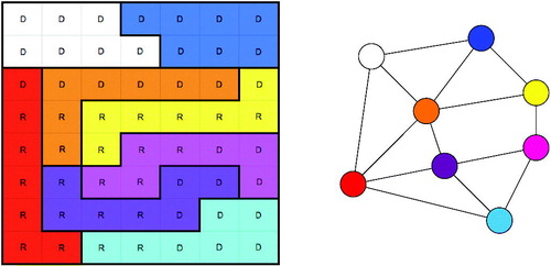
Fig. 2 The districts can be matched the eight different ways listed here, leading to the Democratic party getting anywhere from 25% to 100% of the Senate seats. The two perfect matchings corresponding to the extreme outcomes are shown here.

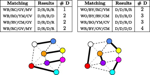
There are exactly eight perfect matchings of this graph; in other words, given these House districts, there are only eight ways to form four Senate districts while respecting nesting. By contrast, there are 2,332,394,150 ways to create four (contiguous, equal-size) Senate districts from these 56 units without that restriction.² If we name the colors White, Blue, Red, Orange, Yellow, Magenta, Cyan, and Violet, we can represent the matchings in the table below.

In this toy example, we discover that the choice of matching can swing the outcome for Democrats from 1 seat to 4 seats out of four. Below, we carry out a similar analysis on real-world data.

1.2 Mathematical Literature on Perfect Matchings

In our motivating example, we considered the Senate outcomes for every possible perfect matching in a small graph. Enumerating all perfect matchings in a given graph is a classical problem in the mathematical field of combinatorics; it has captured significant attention because it is at once quite elementary and extremely difficult to compute for arbitrary graphs (Valiant 1979). The matching problem is also of great interest to physicists studying dimer coverings (domino tilings) of lattices, which are used to estimate thermodynamic behavior of liquids (Kenyon and Okounkov 2005). In 1961, three statistical physicists, Temperley, Fisher, and Kasteleyn, independently and nearly simultaneously derived the formula for the number of perfect matchings of an m × n grid (Kasteleyn 1961; Temperley and Fisher 1961) and subsequently proposed the FKT algorithm for efficiently computing the number of perfect matchings of any planar graph (i.e., in any graph that can be drawn in the plane without edges crossing). The algorithm is discussed in more detail in Appendix B in the supplementary materials. For surveys on the mathematics of matching, see Lovász and Plummer (2009) and Volume A of Schrijver (2003). ³

1.3 Article Outline

The central research question here is to quantify the partisan advantage available to an agent who is empowered only to select a House-to-Senate pairing. In Alaska, where there are only 40 House districts which are patterned in a not very dense manner, it might seem that there is only limited advantage to be gained. However, we will demonstrate that the choice of pairings alone can create a swing of 4–5 seats out of 20 against recent voting patterns. In fact, we will see that even though pairings give a far simpler model of how to create Senate districts, they give just as much partisan latitude as making Senate districts from scratch.

We begin by reviewing pertinent background on Alaska politics, demographics, and redistricting rules in Section 2, culminating in the selection of two recent elections—the Governor and U.S. House races of 2018—to serve as our electoral baselines for the remainder of the analysis. In Section 3, we begin by describing the construction of dual graphs that model the adjacencies of geographical units—in this case, House districts. Next, we overview the algorithmic approaches we apply to those graphs in the rest of the article. These methods include enumerating matchings with a classic algorithm called FKT, constructing sets of matchings with a depth-first algorithm we call prune-and-choose described in Appendix C in the supplementary materials, and finally varying the underlying districts with a Markov chain. The proof of validity for prune-and-choose is found in Appendix C.2 in the supplementary materials.

In the remainder of the article, we report on the results of these algorithmic investigations for Alaska. Beyond the flexibility inherent in choosing the nesting, we find that the interpretation of redistricting rules (in particular, geographic adjacency when regions are connected by water) has a substantial impact on the number of matchings. With the current House districts fixed, Section 4 measures the partisan tilt of the pairing itself among the full set of matchings. Finally, in Section 5, we vary the House and Senate districts themselves by randomly assembling them from precinct building blocks with a method that provides heuristic assurances of representative sampling. By exploring the space of valid plans, and evaluate expected partisan properties and matchability of alternative plans.

In Appendix D in the supplementary materials, we extend this analysis by enumerating the perfect matchings in each of the eight states that mandate two-to-one nesting. For several of these states, it would be computationally infeasible to construct the complete set of matchings because it is prohibitively large; nonetheless, Appendix E in the supplementary materials describes how they can be sampled efficiently.

2 Alaska Electoral Politics

2.1 Partisanship in Alaska

Alaska is an outlier in U.S. political geography for several reasons including its uniquely wide array of viable minor parties featured in both local and statewide races. For example, the state officially recognizes the secessionist Alaskan Independence Party, which succeeded in electing Wally Hickel as Governor in 1990. In addition, there are nine organized “political groups” that are seeking official recognition, and meanwhile are entitled to run candidates for statewide office: the Libertarian, Constitution, Progressive, Moderate, Green, and Veterans Parties, together with the more fringe OWL Party, Patriot’s Party, and UCES Clowns Party.⁴

The current Governor of Alaska is Republican Mike Dunleavy, whose predecessor Bill Walker won as an Independent in 2014, becoming the only sitting U.S. Governor not from one of the two major parties at the time. (Walker had previously left the Republican Party and then successfully ran as an Independent candidate, with a Democratic candidate for Lieutenant Governor.) In 2014, Alaska had the first U.S. Senator in more than 50 years to win election as a write-in candidate, Senator Lisa Murkowski.

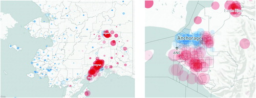
Alaska is also unique in its geographic distribution of the major parties’ strengths. Unlike the contiguous United States, where urban areas tend to be most reliably Democratic, Alaska has Democratic strength in the rural areas to the north and west of the state. These areas are the homes of significant numbers of Native Alaskan residents, who constitutes the largest minority in the state. Conversely, the Republican vote is often stronget in suburban areas. In fact, even the city of Anchorage—by far the most populous in the state with 291,826 out of Alaska’s 710,231 residents in Census 2010—votes Republican overall in recent presidential races, making it a rare city of its size to do so (Figure 3).⁵

Fig. 3 Trump share of major-party Presidential vote per precinct, sized by number of votes cast.

Although it is one of the “reddest” states in national terms, the Republican-Democratic split is not the fundamental divide in Alaskan politics. Extremely conservative Republicans are sometimes balanced by a tenuous coalition of moderate Republicans, Democrats, and Independents, which currently aligns to give net Democratic control in the state House. In 2018, an Independent, Libertarian, or Nonpartisan candidate ran in nine of the 40 House districts; an Independent won in one district and one Democratic candidate changed his affiliation to undeclared after winning (Ballotpedia 2019). In areas where the Democratic party label is an obstacle to election, running as an Independent can be a successful political strategy. The majority caucus in the House originally consisted of 25 members: all 15 Democrats, the two unaffiliated members, and eight Republicans (Ballotpedia 2019).⁶ On the other hand, one state Senator elected as a Democrat caucuses with the Republican majority in that body (Alaska Senate Majority Profile n.d.).

2.2 Racial Demographics and the Voting Rights Act

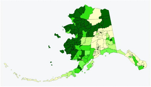
The 2010 Census reports Alaska’s racial demographics as roughly 6% Hispanic, with non-Hispanic population comprising 63% White, 3.5% Black, 5.5% Asian, and 15% Alaska Native or other Native American as shares of the total. An additional 9% of residents are recorded as belonging to other races, or to two or more races. Figure 4 shows the proportion of Alaska Native or other Native American residents across the state.

Fig. 4 Proportion of Alaska Native or other Native American residents across Alaska. The color scale is in equal intervals of 20%; the darkest shade marks precincts that are 80–100% Native.

The large Alaska Native population has long been singled out for federal protection under the Voting Rights Act of 1965, specifically Section 5 of the VRA, which required covered jurisdictions to seek prior federal approval (or “preclearance”) for any changes to districts or other voting laws. Alaska’s inclusion owed to a long history of discriminatory “literacy tests”—in this case, English-language tests used to deny voting eligibility to Native residents—making Alaska one of only nine states covered in full by the special protections (U.S. Department of Justice 2015).⁷ Though the Supreme Court ended the practice of preclearance with Shelby v. Holder (2013), all states are still bound by the VRA requirement to afford minority groups the ability to elect a candidate of their choice where possible.⁸ Issues of fair representation and ballot access for the rural Native population are still highly active in Alaska (Caldwell 2013).

2.3 Redistricting Rules and Practices

Following a 1998 state constitutional amendment, a five-member Alaska Redistricting Board was formed to draw new district lines after each decennial census (Epler 2011). The House speaker, Senate president, and Chief Justice of the state Supreme Court each choose one member of the board, and the Governor chooses two. At least three members of the board must approve a redistricting plan for it to be adopted. The board must draw maps in accordance with the state Constitution, which requires that House districts be “contiguous and compact territory containing as nearly as practicable a relatively integrated socio-economic area… [and] contain[ing] a population as near as practicable to the quotient obtained by dividing the population of the state by forty” while Senate districts are simply “…composed as near as practicable of two contiguous house districts” without further constraints (State Constitution of Alaska n.d.).⁹

Balancing the requirements of the VRA and the guidelines of the state Constitution—compactness in particular—means that Alaska’s House and Senate districts have to be drawn in a coordinated fashion in most of the state. However, Alaska’s relatively urban centers of Anchorage and Fairbanks are both predominantly white and made up of small, regular pieces. This homogeneity of demographics and geography provides additional flexibility in these regions for the map drawer to construct House districts first, without considering potential Senate pairings.

Allegations of partisan intent have frequently been leveled at the redistricting process in Alaska. The maps drawn after the 2000 Census were accused of being a Democratic gerrymander, while Democrats have called the post-2010 maps (drawn by a board with a 4–1 Republican majority) a Republican gerrymander (Mauer 2013). The fact that a Democratic-led caucus controls the House while Republicans have 2/3 control of the Senate lends credence to the possibility that not the House districts themselves, but their pairing to form Senate districts, is chosen for Republican advantage. That possibility is investigated below.

2.4 Our Choice of Election Data

In Alaska, three types of races occur statewide. The entire state votes for a Governor and Lieutenant Governor, elected on a single ticket, every four years; they elect one member to the U.S. House of Representatives every two years; and they elect a U.S. Senator for a term of 6 years in the Class 2 and Class 3 cycles.

We consider only those elections which occurred after the implementation of new maps in July 2013. (A map approved for temporary use in 2012 was replaced after litigation.) Seven statewide races occurred in this time period:

Table

Gov14	Walker (I/D)	[48.10%]	Parnell (R)	[45.88%]
Cong14	Young (R)	[50.97%]	Dunbar (D)	[40.97%]
			McDermott (L)	[7.61%]
Sen14	Sullivan (R)	[47.96%]	Begich (D)	[45.83%]
Cong16	Young (R)	[50.32%]	Lindbeck (D)	[36.02%]
			McDermott (L)	[10.31%]
Sen16	Murkowski (R)	[44.36%]	Miller (L)	[29.16%]
			Stock (I)	[13.23%]
			Metcalfe (D)	[11.62%]
Cong18	Young (R)	[53.08%]	Galvin (D)	[46.50%]
Gov18	Dunleavy (R)	[51.44%]	Begich (D)	[44.41%]

The list includes all candidates with at least 5% of the vote in any race. ¹⁰

We will use the Cong18 and Gov18 races as the fundamental electoral data for the analysis below. These two contests feature a Democratic and Republican candidate without major third-party presence and are interesting because they have very different spatial patterns of party support but similar bottom-line partisan shares. The two-party vote share for the Democrat in those races was 46.7% for Alyse Galvin against Don Young for Congress and 46.3% for Mark Begich against Mike Dunleavy for Governor. ¹¹

Alaskan elections receive a high proportion of ballots not reported through individual precincts. These unprecincted ballots include absentee, provisional, and early votes, which are all reported by legislative House district. For federal races such as the U.S. House, a small number of overseas military ballots are also reported on a statewide basis. In the 2018 U.S. House race, 33.36% of reported ballots were unprecincted. In the 2018 Governor race, 34.18% of ballots were unprecincted. (For ease of reference, we will call all unprecincted ballots “absentee” below.) We report results for each election both including and excluding the absentee ballots. Thus, our four election treatments can be labeled Gov18-N, Gov18-A, Cong18-N, and Cong18-A, where the N versions drop absentee ballots from the tally and the A versions include them (Figure 5). In Section 5, we need to know the precinct location of the votes; for this, we assign absentee ballots to precincts in numbers proportional to precinct population.

Fig. 5 These choropleth images show that party preferences in the Governor race are spatialized very differently from the U.S. House race, even though the statewide party share is nearly identical. On the other hand, there is little visible change with and without including absentee ballots (marked with A and N, respectively), though this does have a significant bottom-line partisan impact.

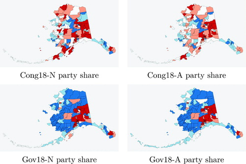
Table 1 shows clearly that absentee ballots collectively favor Democrats by roughly two percentage points per House district. Only districts 37 and 38 have a Republican lean in the absentee ballots in either election.

Table 1 How the currently enacted House and Senate districts fall with respect to the voting patterns from our two selected elections.

NOTE: The individual rows correspond to the 40 numbered state House districts, paired into the 20 state Senate districts labeled A–T. The highlighting in the votes columns shows which party received the majority of the two-way vote share in the corresponding Senate district.

3 Data and Methods

All experiments in this article were performed on an Ubuntu 16.04 machine with 64 GB memory and an Intel Xeon Gold 6136 CPU (3.00 GHz). Algorithmic descriptions of the FKT method for enumerating matchings and the Prune-and-Choose method for generating matchings are given in Appendices B and C of the supplementary materials, respectively.

3.1 Election Results, Shapefiles, and Dual Graphs

Election data were gathered from the Alaska elections website (Alaska Division of Elections n.d.) and demographic data were obtained from the 2010 Census. Absentee and early voting information was only available by House district, so precinct-level data was assigned by prorating by population. We prepared the geospatial data with the MGGG Preprocessing Suite, which uses areal interpolation for blocks not fully contained in precincts (Metric Geometry and Gerrymandering Group 2019b). The cleaned and processed version of the data is available on GitHub (Metric Geometry and Gerrymandering Group 2018b).

In the 2010 Census, Alaska had 45,292 census blocks, of which over a third (18,263) are water-only. Alaska has 441 precincts, ranging in population from a minimum of 44 people (Pedro Bay) to 7994 people (JBER1, in Anchorage) (Alaska Division of Elections n.d.). Six precincts have over 5000 people, and 16 have under 100.

Beginning with a shapefile of the geography, in this instance precincts, we use geospatial libraries in Python to create a dual graph in GerryChain whose nodes are the geographic units, and where two units are connected by an edge if their units share a positive-length boundary in the shapefile (Metric Geometry and Gerrymandering Group 2018a). We then adjust edges to better correspond to plausible notions of adjacency, especially when water is involved, as described below.

3.1.1 Water Adjacency

For areas connected only by water, a decision must be made about whether to count them as adjacent. To illustrate the impact of this seemingly minor issue, we construct three different dual graphs of the precinct map, which we call the tight, restricted, and the permissive graphs.

Permissive adjacency is the closest match to the AK Division of Elections precinct shapefile. The dual graph of those precincts is nearly connected using this approach, except for one gap in the Kodiak archipelago and five additional island precincts of the West coast. We manually added all visually reasonable connections in these cases. Among the 441 precincts, this process produces 1151 edges. Aggregating the precincts into the 40 current House districts produces a House district dual graph with 100 edges.

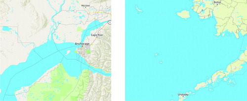
To construct our more restricted notion of adjacency, we consulted the Census Bureau Cartographic Boundary shapefile, which is clipped to land, that is, excludes water from its geographic units. With this as a guide, we removed certain connections across water (see Figure 6). This reduces the number of edges modestly, from 1151 to 1109 for the precinct dual graph and from 100 to 92 for the House dual graph.

Fig. 6 The Cook Inlet is a body of water stretching up from the Gulf of Alaska; its Knik Arm and Turnagain Arm surround the densest part of Anchorage, separating it from rural precincts to the north and south. Following precinct adjacencies provided by the state would allow districts to jump across the water, while a more restrictive notion of adjacency would not. On the right, we see that the precinct shapefile gives no guidance on how the islands are allowed to be connected to the mainland by districts.

Finally, we create the tightest version of the graph by using the current House map as a guide, keeping the fewest water adjacencies that would allow the current districts to be considered valid. This gives us a tight dual graph with 1105 precinct edges and 89 House edges. As we will see below, these small changes to the underlying dual graph can have large consequences for the number of possible matchings. Figure 7 shows the resulting graphs, which we use in the remainder of the analysis.

Fig. 7 The three Alaska dual graphs.

3.2 Markov Chains for Generating Alternative House Plans

Markov chain Monte Carlo, or MCMC, is the leading method in scientific computing for searching large spaces and studying properties of complex systems. Numerous research groups now use MCMC implementations to study the universe of possible districting plans, once the basic units have been set (Bangia et al. 2017; Chikina, Frieze, and Pegden 2017; DeFord, Duchin, and Solomon 2019). We use the open-source software package GerryChain, created by the Voting Rights Data Institute (Metric Geometry and Gerrymandering Group 2018a).

This algorithm generates new plans iteratively, making modifications to the districting assignments of some of the units at each step. To choose how to modify districts at random, we use a proposal called Recombination (ReCom), introduced in DeFord, Duchin, and Solomon (2019).¹² At each step, this proposal merges the units of two adjacent districts and then uses a balanced cut of a spanning tree to generate a new division of the merged districts. The user can elect to impose hard constraints in the form of requirements for plans, or can choose a weighted random walk that preferentially selects plans with properties deemed to better comport with the districting principles. The tree method itself promotes the selection of compact districts, so the plans generated in this way tend to have comparable compactness statistics to human-approved plans and to comfortably pass the “eyeball test” for district shape.

We ran our Markov chains on Alaska’s 441 precincts as basic units, seeking new legally valid plans for forming them into 40 House districts. As outlined in Section 2.3, the law requires that the districters aim to produce equipopulous, compact, and contiguous districts.

The ideal population of a House district is 710,231/40, or between 17,755 and 17,756 people. By federal law and common practice, legislative districts can deviate by up to 5% from ideal size without a special reason, so we have imposed that limit on population balance, allowing 16,868–18,643 people per district. The same level of population balance was imposed on the Senate ensembles.

We generated ensembles of 100,000 distinct House and Senate districting plans, varying the definitions of contiguity (tight/restricted/permissive). A district-level dual graph of the sampled plan was pulled every step. Using FKT, we counted the number of matchings for each districting plan and edges between House districts, and we stored plans with extreme matching statistics. The goal was to learn whether the new plans could have markedly different partisan outcomes, either on their own or when matched to form a Senate plan, from the current districts.

Replication code for producing and analyzing these ensembles is available on GitHub (Metric Geometry and Gerrymandering Group 2019a).

4 Alternative Matchings in Current House Plan

In this section, we evaluate the currently enacted House plan by generating all of the potential matchings and computing their partisan behavior under our chosen election data. We start by computing the number of matchings for each of our notions of adjacency, reported in Table 2, using the FKT algorithm described in Appendix B in the supplementary materials. This already highlights the fact that toggling a small number of edges in the Alaska House dual graph (due only to reasonable interpretations of water adjacency) can change the number of perfect matchings very substantially; in this case, the number of matchings jumps by nearly a factor of eight.¹³

Table 2 On Alaska, FKT (which only counts matchings) runs in a fraction of a second; the prune-and-choose algorithm (which stores matchings) runs in under 2 min.

Alaska	Tight	Restricted	Permissive
Dual edges	89	92	100
Matchings	14,446	29,289	108,765
FKT runtime	0.022 sec	0.022 sec	0.027 sec
Prune–and–choose runtime	14.2 sec	28.5 sec	105.1 sec

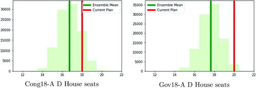
We then use the prune-and-choose algorithm described in Appendix C in the supplementary materials to generate each of the possible pairings. For each matching, we evaluate its performance under each of the four election treatments, comparing the number of Senate districts with a Democratic majority in the actual plan to the average number over the Senate plans formed by all possible matchings (Table 3). It bears emphasizing that the Democratic seats reported across the table refers to the number of Senate districts in which Galvin votes outnumbered Young votes for Congress, or Begich votes outnumbered Dunleavy votes for Governor.

Table 3 Partisan outcome and competitiveness in the current (Enacted) Senate plan compared to the average over alternative matchings.

	D Senate districts
	Enacted	Tight	Restricted	Permissive
Cong18-N	6	6.90	6.78	6.52
Cong18-A	7	8.30	8.18	7.93
Gov18-N	7	7.69	7.57	7.33
Gov18-A	7	8.24	8.13	7.88

Table 3 continue

	Competitive districts
	Enacted	Tight	Restricted	Permissive
Cong18-N	13	12.12	11.90	11.91
Cong18-A	12	12.33	12.26	12.54
Gov18-N	11	10.54	10.55	10.21
Gov18-A	10	9.78	9.68	9.68

NOTE: A competitive district is defined here as one with a D share between 40% and 60%. Here, every partisan outcome is more favorable to Republicans than the neutral expectation. Compare Table 4, which varies the underlying House plan and shows the opposite partisan tendency.

Comparing the enacted plan against all possible pairings does indeed find a small Republican tilt, falling approximately one seat to the Republican side of the typical matching but certainly does not appear to be a significant outlier.¹⁴ (At the same time, we can observe the substantial effect of discarding absentee ballots: it shifts outcomes toward Republicans by about 1 seat.) The histograms in Figure 8 add detail by showing the full distribution of Democratic seats with respect to each race.

Fig. 8 The number of Senate districts with a D majority, as the matching varies across the permissive set. The blue line marks the average number of Democratic seats over all matchings and the red line shows the outcome in the current plan, showing a one-seat advantage for Republicans in the current matching and a four- to five-seat swing overall. These two histograms look nearly identical for the different elections, despite the substantial differences in how the vote was distributed.

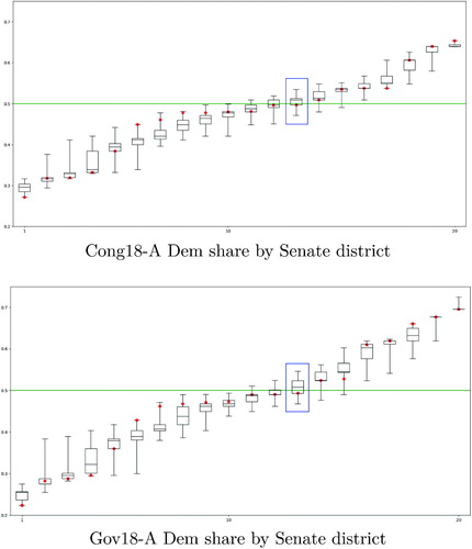
For even more granular detail, at the level of individual districts, we can study box-and-whisker plots (Figure 9). In these images, the districts are ordered from lowest to highest Democratic vote share to make them comparable over the ensembles. The boxes show the 25th–75th percentile range and the whiskers show every result achieved over the full set of (permissive) matchings. Similar histograms and boxplots for the remainder of the elections and dual graphs are available in our supplementary materials (Metric Geometry and Gerrymandering Group 2019a).

Fig. 9 Democratic vote share in current Senate districts (red dots), compared to range in comparable districts over the full set of matchings (box and whiskers). With district-by-district detail, the differences between the two elections’ voting patterns are more visible. For instance, the 13th-indexed districts in the state have a Galvin (Congressional) share and a Begich (Governor) share just under the median of the respective ensembles, while nearly 75% of the ensemble in each case had a Democratic majority in the corresponding district. Where boxes have degenerated to a single value, it is because some matchings are forced, thinning the number of possibilities.

5 Alternative House and Senate Districts

5.1 Partisan Outcomes

Using the Markov chain ensembles of 100,000 plans each as a neutral counterfactual for drawing districts, we first report the number of House districts out of 40 with more Democratic than Republican votes (Table 4).

Table 4 The number of House districts with a D majority and the number of competitive districts, as the House plan varies.

	D House districts
	Enacted	Tight	Restricted	Permissive
Cong18-N	15	14.10	13.93	14.28
Cong18-A	18	16.35	16.33	16.73
Gov18-N	15	14.73	14.55	14.44
Gov18-A	20	17.86	17.63	17.65

Table 4 continue

	Competitive districts
	Enacted	Tight	Restricted	Permissive
Cong18-N	24	25.51	25.01	25.23
Cong18-A	24	24.85	24.62	24.88
Gov18-N	19	21.03	20.60	20.59
Gov18-A	19	20.83	20.57	20.52

NOTE: A competitive district is defined as one in which the D share is between 40% and 60%. Compare Table 3.

Beyond the averages, we can view the full histograms to gauge the extent to which the current plan is an outlier (Figure 10).

Fig. 10 The number of districts with a D majority in the indicated election, over the ensemble of (permissive) House plans.

Recall that the current majority House caucus includes 24 members: 16 members who were elected as Democrats, seven members who were elected as Republicans, and one who was elected as an Independent.

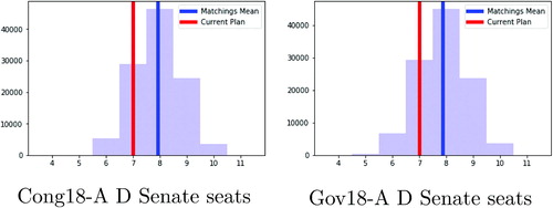
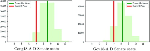
The Senate ensemble gives another interesting vantage point. With respect to both vote patterns, the bulk of plans assembled by the Markov chain process have 7–10 Democratic Senate seats, and the full range observed in the ensemble is 6–11 (Figure 11). Compare this to simply matching the current House plan, where we can fully exhaust the possibilities instead of sampling. Matchings give us Democratic seat outcomes of 6–10 in either vote pattern, with a small number that achieve a 5-seat outcome against the Governor returns. This means that mere control over the matchings gives essentially just as much partisan latitude as the right to draw plans from scratch with the most permissive notion of precinct adjacency.

Fig. 11 The number of districts with a D majority in the indicated election, over the ensemble of (permissive) Senate plans.

5.2 Native Population

We also find that the number of districts with an Alaska Native population majority is typically 3–4 in our randomly produced House plans, compared to three in the current House plan. Furthermore, the ability to form districts more permissively across water makes a very noticeable difference, boosting the likelihood of forming a fourth majority-Native district by random selection.

Table

Number of majority-Native House districts	2	3	4
Permissive ensemble	444	53,596	45,960
Restricted ensemble	1053	97,069	1878
Tight ensemble	1135	97,507	1358

5.3 Rematching the New Plans

Over each ensemble of 100,000 House plans, we computed the number of dual edges and the number of perfect matchings. The (nonzero) numbers of matchings varied from 74 to 165,344 (tight), 42 to 194,588 (restricted), and 852 to 961,176 (permissive). To a first approximation, more edges means more matchings, but the scatterplots in Figure 12 show that there is also substantial dependence on the specific placement of the edges.¹⁵

Fig. 12 The relationship between the number of edges (x axis) and the number of matchings (y axis). Each point is a House plan, varying over the tight (top left), restricted (lower left), and permissive (right) ensembles.

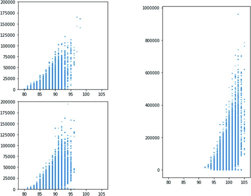
To illustrate the sensitive dependence of the number of matchings on the precise topology of the graph, we focus on three examples found in the permissive House ensembles in Figure 13. The leftmost dual graph has 103 edges and 961,176 matchings while the next one has more edges but less than half the number of matchings. The disparity in these matching counts is almost entirely due to the fact that there are two ways to pair the districts in the “panhandle” of the 103-edge graph—[(29,30), (39,40)], or [(29,39), (30,40)]—compared to the unique pairing [(17,40), (35,36)] in the corresponding region of the 105-edge graph. This accounts for a doubling in the number of overall matchings, assuming a comparable number of ways to match the remaining 36 vertices. Forced pairings play an important role in plans with few matchings. The rightmost graph shows an example with 101 edges but only 852 matchings, the lowest nonzero number ever observed. This is due to the many forced pairs—[(11,13), (12,34), (2,3), (1,36), (4,33), (8,24), (7,26), (17,25)]—which limits the flexibility in pairing the remaining vertices.

Fig. 13 A selection of three House plans from our ensembles whose dual graphs have various extremal properties. The violin plot shows the number of Democratic districts with respect to Gov18-A vote data, and the colored regions show the relative sizes of the matching sets.

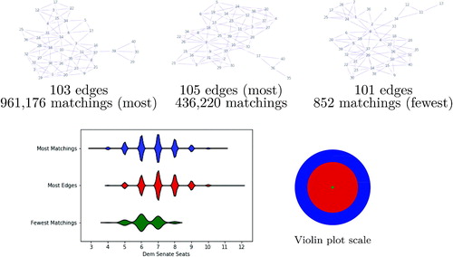
The analysis demonstrates that the matchability of the underlying House plan can have a significant downstream partisan impact on the Senate plans that can be formed. Figure 13 shows examples of this behavior by comparing the distributions over the possible perfect matchings for three plans from the permissive ensemble. For each of the three House plans, a typical perfect matching has 5–8 Democratic districts out of 20. However, by choosing a House plan with more district adjacencies or more matchings, it is possible to get as few as 3 or as many as 12. Investigating the full flexibility allowed to a mapmaker who controls the House district drawing process is an interesting question for further research.

6 Conclusions

Numerous studies have sought to quantify the partisan advantage secured by the selection of a particular districting plan. In that vein, we find that the current Alaska House plan favors Democrats by an estimated 1–2 seats out of 40 when compared to other (contiguous, compact, population-balanced) ways of forming districts from precincts. The core of the article, however, is a novel application of rigorous mathematics to redistricting in the case of a nesting rule for state legislatures. For that, we can apply the theory of perfect matchings of graphs, learning that the Alaska Senate plan secures a Republican advantage of 1 seat out of 20 when compared to other ways to match the House districts. Other findings:

• The choice of matching of a fixed House plan gives as much latitude to control partisan outcomes as drawing a Senate plan from scratch: approximately a five-seat swing out of 20.

• The significant number of absentee/early/provisional ballots in Alaska skew markedly Democratic. Different choices of how to assign them to precincts will impact findings about the consequences of moving district boundaries, and should be further studied. However, this has no effect on our analysis of matchings.

• Well-chosen statewide races, in this case the 2018 Governor and Congressional elections, gave partisan measurements that are closely compatible with each other and qualitatively concordant with the Legislative outcomes.

• Contiguity rules are not completely straightforward, and can have a major role in shaping the space of districting possibilities. For instance, permissive water adjacency makes nearly half of neutrally generated House plans have a fourth majority-Native district, while less than 2% of plans do with more restricted adjacency (Section 5.2).

Supplementary Materials

The supplement contains additional plots and technical descriptions of the algorithms used in the article for enumerating and sampling perfect matchings. Appendix A shows reference figures of the state House dual graphs for the states with strict nesting rules (besides Alaska). Further information about the FKT algorithm is given in Appendix B; Appendix C introduces the PruneandChoose algorithm and provides a proof of correctness. In Appendix D, these algorithms are applied to all states with a nesting rule to compare the relative sizes of the sets of matchings. Finally, in Appendix E we implement and validate a uniform sampling procedure for matchings that can be applied even in the states where generating all of the matchings would be computationally infeasible.

Acknowledgments

SG thanks David P. Williamson and Kenrick Bjelland for helpful discussions. We thank Coly Elhai, Mallory Harris, Claire Kelling, Samir Khan, and Jack Snoeyink for substantial joint work and conversations on other approaches to modeling Alaska redistricting, and particularly acknowledge Samir Khan for his initial implementation of prune-and-choose. Hakeem Angulu, Ruth Buck, and Max Hully provided excellent data and technical support. Finally, we thank Anchorage Assemblyman Forrest Dunbar for bringing this problem to our attention.

Additional information

Funding

The authors acknowledge the Prof. Amar G. Bose Research Grant at MIT and the Jonathan M. Tisch College of Civic Life at Tufts University for ongoing support. MD is partially supported by NSF DMS-1255442. SG is partially supported by NSF DGE-1650441.

Notes

1 The article of the Ohio constitution with this requirement was in effect in 2011 but has now been repealed, effective 2021.

2 This is the number of partitions of a 7 × 8 grid graph into four contiguous “districts” of 14 nodes each. See mggg.org/table.html for a discussion of enumeration patterns for districting problems on grids, and a link to enumeration code.

3 This problem is also intimately related to a second enumeration problem, that of counting the spanning trees of a graph. The number of spanning trees is sometimes called the complexity of a graph. Temperley defined a transformation that starts with a graph and creates a new associated graph called its T-graph. A series of remarkable theorems tell us that if G is the T-graph associated to $\overline{G}$ , then the number of spanning trees of $\overline{G}$ is exactly equal to the number of perfect matchings of G (Temperley 1974; Burton and Pemantle 1993; Kenyon 2000; Kenyon, Propp, and Wilson 2000).

4 See http://www.elections.alaska.gov/Core/politicalgroups.php.

5 In the 2016 Presidential race, Trump’s share of the major party vote was 58.4% statewide and 53.1% in Anchorage. The trend holds up across elections in the last cycle, with Republican performance in Anchorage trailing statewide levels by only about four points.

6 Twenty-one members (15 Democratic, 4 Republican, and two unaffiliated) voted together to elect the current Speaker (who ran for his House seat as a Democrat but became unaffiliated just days before being elected Speaker). Four more Republicans joined to establish the majority caucus. In May 2019, however, one Republican left the House majority coalition (Associated Press 2019; Ballotpedia 2019)

7 Since 1971, the indigenous people of Alaska are organized into thirteen regional Tribal Corporations to administer land and finances. The current legal landscape gives the corporations substantial financial clout, which does not translate to commensurate political representation for the broader Native Alaskan population.

8 State courts have established that Alaska redistricters must consider the state’s constitutional requirements for districts before considering the requirements of the Voting Rights Act. Alaska’s courts have enforced this hierarchy several times, including most recently in a 2012 ruling that invalidated the maps used in that year’s elections (Mauer 2013).

9 As far as we are aware, the socio-economic clause has never been operationalized or enforced.

10 Walker ran for Gov14 as an Independent, but with a Democratic running mate. In Gov18, Walker dropped out and ultimately received just 2% of the vote.

11 We note that the question of preferring endogenous or exogenous election data for redistricting analysis is a live one in political science, as reflected for instance in the article, rejoinder, and response between Best et al. and McGhee in the March 2018 issue of the Election Law Journal (Best et al. 2017a, 2017b; McGhee 2017). Our research group inclines to the use of well-chosen exogenous (statewide) election data in general, but we further note that using endogenous data would be forbidding in the Alaska legislature. Besides a significant number of uncontested races, these legislative races also feature a proliferation of minor parties (described above), making a regression analysis particularly inadequate to cleanly model voters’ preferences between the two major parties.

12 The scientific advantage of using Markov chains to sample districting plans is that they have a theoretical guarantee of producing representative samples (with respect to their stationary disributions) if run for long enough. In our case, we run the chains until we obtain strong heuristic evidence of mixing, which is a common and effective standard in scientific computing. See DeFord, Duchin, and Solomon (2019).

13 It is worth emphasizing that the number of matchings is sensitively dependent on the precise edge structure as well as simply the number of edges. This fact is explored below in Section 5.3.

14 The actual Senate composition also has six or seven Democrats, depending on how you count: seven state Senators were elected as Democrats, but Sen. Lyman Hoffman caucuses with the Republican majority.

15 One notable feature of Figure 12 is the prevalence of plans with low numbers of matchings. It is easy to construct graphs with any number of edges and zero matchings, simply by having any two leaves (vertices of degree one) connected to a single common neighbor—and this can easily occur by chance. There were no matchings at all in 2319, 4274, and 3504 of the dual graphs found by the ensembles, respectively. It is similarly easy to randomly construct graphs with very few matchings simply by having many leaves and thus many forced edges. On the other hand, there are graphs with 2n vertices, roughly $n^2/2$ edges, and only a single matching: start with a complete graph on n vertices (i.e., with all edges present) and add a single leaf connected to each of those. Each leaf vertex is forced to match to its unique neighbor, leaving no more vertices to pair.

References

- Alaska Division of Elections (n.d.), “Research Information,” available at http://www.elections.alaska.gov/doc/info/ElectionResults.php.
- Alaska Senate Majority Profile (n.d.), “Senator Lyman Hoffman,” available at https://www.alaskasenate.org/2018/member/lyman-hoffman/.
- Associated Press (2019), “LeDoux Stripped of Assignments After Break With Caucus,” available at https://www.apnews.com/2ab3db7cbe1448abae74989d8f2785fb.
- Ballotpedia (2019), “Alaska House of Representatives Elections 2018,” available at https://ballotpedia.org/Alaska_House_of_Representatives_elections_2018.
- Bangia, S., Graves, C. V., Herschlag, G., Kang, H. S., Luo, J., Mattingly, J. C., and Ravier, R. (2017), “Redistricting: Drawing the Line,” arXiv no. 1704.03360.
- Best, R. E., Donahue, S. J., Krasno, J., Magleby, D. B., and McDonald, M. D. (2017a), “Authors’ Response Values and Validations: Proper Criteria for Comparing Standards for Packing Gerrymanders,” Election Law Journal: Rules, Politics, and Policy, 17, 82–84. DOI: 10.1089/elj.2017.0471.
- Best, R. E., Donahue, S. J., Krasno, J., Magleby, D. B., and McDonald, M. D. (2017b), “Considering the Prospects for Establishing a Packing Gerrymandering Standard,” Election Law Journal: Rules, Politics, and Policy, 17, 1–20.
- Burton, R., and Pemantle, R. (1993), “Local Characteristics, Entropy and Limit Theorems for Spanning Trees and Domino Tilings Via Transfer-Impedances,” The Annals of Probability, 21, 1329–1371. DOI: 10.1214/aop/1176989121.
- Caldwell, S. (2013), “Voting Rights Act: What Does Ruling Mean for Alaskans?,” Anchorage Daily News, available at https://www.adn.com/politics/article/supreme-court-decision-voting-rights-may-ease-alaska-redistricting-work/2013/06/25/.
- Chikina, M., Frieze, A., and Pegden, W. (2017), “Assessing Significance in a Markov Chain Without Mixing,” Proceedings of the National Academy of Sciences of the United States of America, 114, 2860–2864. DOI: 10.1073/pnas.1617540114.
- DeFord, D., and Duchin, M. (2019), “Redistricting Reform in Virginia: Districting Criteria in Context,” Virginia Policy Review, 12, 120–146.
- DeFord, D., Duchin, M., and Solomon, J. (2019), “Recombination: A Family of Markov Chains for Redistricting,” arXiv no. 1911.05725.
- Epler, P. (2011), “Alaska Redistricting Board Gets to Work,” Anchorage Daily News, available at https://www.adn.com/alaska-news/article/alaska-redistricting-board-gets-work/2011/03/17/.
- Kasteleyn, P. W. (1961), “The Statistics of Dimers on a Lattice: I. The Number of Dimer Arrangements on a Quadratic Lattice,” Physica, 27, 1209–1225. DOI: 10.1016/0031-8914(61)90063-5.
- Kenyon, R. (2000), “The Asymptotic Determinant of the Discrete Laplacian,” Acta Mathematica, 185, 239–286. DOI: 10.1007/BF02392811.
- Kenyon, R., and Okounkov, A. (2005), “What Is a Dimer?” Notices of the AMS, 52, 342–343.
- Kenyon, R., Propp, J., and Wilson, D. (2000), “Trees and Matchings,” The Electronic Journal of Combinatorics, 7, R25. DOI: 10.37236/1503.
- Levitt, J. (2008), “A Citizen’s Guide to Redistricting,” Brennan Center Report.
- Lovász, L., and Plummer, M. D. (2009), Matching Theory (Vol. 367), Providence, RI: American Mathematical Society.
- Mauer, R. (2013), “Judge Scolds Alaska Redistricting Board,” Anchorage Daily News.
- McGhee, E. (2017), “Rejoinder to ‘Considering the Prospects for Establishing a Packing Gerrymandering Standard’,” Election Law Journal: Rules, Politics, and Policy, 17, 73–82. DOI: 10.1089/elj.2017.0461.
- Metric Geometry and Gerrymandering Group (2018a), “GerryChain,” GitHub Repository, available at https://github.com/mggg/gerrychain.
- Metric Geometry and Gerrymandering Group (2018b), “MGGG-States,” GitHub Repository, available at https://github.com/mggg/mggg-states.
- Metric Geometry and Gerrymandering Group (2019a), “Alaska,” GitHub Repository, available at https://github.com/mggg/Alaska.
- Metric Geometry and Gerrymandering Group (2019b), “Maup,” GitHub Repository, available at https://github.com/mggg/maup.
- Schrijver, A. (2003), Combinatorial Optimization: Polyhedra and Efficiency (Vol. 24), Berlin, Heidelberg: Springer-Verlag.
- State Constitution of Alaska (n.d.), “Article 6—Legislative Apportionment.”
- Temperley, H. N. V. (1974), “Enumeration of Graphs on a Large Periodic Lattice,” in Combinatorics (Proc. British Combinatorial Conf., Univ. Coll. Wales, Aberystwyth, 1973), Lecture Note Ser. No. 13, London, UK: London Mathematical Society, pp. 155–159.
- Temperley, H. N. V., and Fisher, M. E. (1961), “Dimer Problem in Statistical Mechanics—An Exact Result,” The Philosophical Magazine: A Journal of Theoretical Experimental and Applied Physics, 6, 1061–1063. DOI: 10.1080/14786436108243366.
- U.S. Department of Justice (2015), “Preclearance,” available at https://www.justice.gov/crt/jurisdictions-previously-covered-section-5.
- Valiant, L. G. (1979), “The Complexity of Computing the Permanent,” Theoretical Computer Science, 8, 189–201. DOI: 10.1016/0304-3975(79)90044-6.