The Essential Role of Empirical Validation in Legislative Redistricting Simulation

ABSTRACT

As granular data about elections and voters become available, redistricting simulation methods are playing an increasingly important role when legislatures adopt redistricting plans and courts determine their legality. These simulation methods are designed to yield a representative sample of all redistricting plans that satisfy statutory guidelines and requirements such as contiguity, population parity, and compactness. A proposed redistricting plan can be considered gerrymandered if it constitutes an outlier relative to this sample according to partisan fairness metrics. Despite their growing use, an insufficient effort has been made to empirically validate the accuracy of the simulation methods. We apply a recently developed computational method that can efficiently enumerate all possible redistricting plans and yield an independent sample from this population. We show that this algorithm scales to a state with a couple of hundred geographical units. Finally, we empirically examine how existing simulation methods perform on realistic validation datasets.

KEYWORDS:

• Enumeration
• Gerrymandering
• Graph partition
• Markov chain Monte Carlo
• Redistricting
• Zero-suppressed binary decision diagram

1 Introduction

Congressional redistricting, which refers to the practice of redrawing congressional district lines following the constitutionally mandated decennial census, is of major political consequence in the United States. Redistricting reshapes geographic boundaries and those changes can have substantial impacts on representation and governance in the American political system. As a fundamentally political process, redistricting has also been manipulated to fulfill partisan ends, and recent debates have raised possible reforms to lessen the role of politicians and the influence of political motives in determining the boundaries of these political communities.

Starting in the 1960s, scholars began proposing simulation-based approaches to make the redistricting process more transparent, objective, and unbiased (early proposals include Vickrey 1961; Weaver and Hess 1963; Hess et al. 1965; Nagel 1965). While this research agenda lay dormant for some time, recent advances in computing capability and methodologies, along with the increasing availability of granular data about voters and elections, has led to a resurgence in proposals, implementations, and applications of simulation methods to applied redistricting problems (e.g., Cirincione, Darling, and O’Rourke 2000; McCarty, Poole, and Rosenthal 2009; Altman and McDonald 2011; Chen and Rodden 2013; Fifield et al. 2014; Fifield, Higgins, et al. 2020; Mattingly and Vaughn 2014; Liu, Tam Cho, and Wang 2016; Herschlag, Ravier, and Mattingly 2017; Chikina, Frieze, and Pegden 2017; Magleby and Mosesson 2018; Carter et al. 2019; DeFord, Duchin, and Solomon 2019).

Furthermore, simulation methods for redistricting play an increasingly important role in court cases challenging redistricting plans. In 2019, simulation evidence was introduced and accepted in redistricting cases in North Carolina, Ohio, and Michigan.¹ In the few years prior, simulation methods were presented to courts in North Carolina, and Missouri.² Given these recent court cases challenging redistricting in state and federal courts, simulation methods are expected to become an even more influential source of evidence for legal challenges to redistricting plans across many states after the upcoming decennial census in 2020.

These simulation methods are designed to yield a representative sample of redistricting plans that satisfy statutory guidelines and requirements such as contiguity, population parity, and compactness.³ Then, a proposed redistricting plan can be considered gerrymandered if it constitutes an outlier relative to this sample according to a partisan fairness measure (see Katz, King, and Rosenblatt 2020, for a discussion of various measures). Simulation methods are particularly useful because enumeration of all possible redistricting plans in a state is often computationally infeasible. For example, even partitioning cells of an 8 × 8 checkerboard into two connected components generates over $1.2\times {10}^{11}$ unique partitions (see https://oeis.org/A068416). Unfortunately, most redistricting problems are of much greater scale.⁴ Therefore, to compare an implemented redistricting plan against a set of other candidate plans, researchers and policy makers must resort to simulation methods.

Despite the widespread use of redistricting simulation methods in court cases, insufficient efforts have been made to examine whether or not they actually yield a representative sample of all possible redistricting plans in practice.⁵ Instead, some assume that the existing simulation methods work as intended. For example, in his amicus brief to the Supreme Court for Rucho et al. v. Common Cause, Eric Lander declares,⁶

With modern computer technology, it is now straightforward to generate a large collection of redistricting plans that are representative of all possible plans that meet the State’s declared goals (e.g., compactness and contiguity).

And yet, if there exists no scientific evidence that these simulation methods can actually yield a representative sample of valid redistricting plans, we cannot rule out the possibility that the comparison of a particular plan against sampled plans yields misleading conclusions about gerrymandering.

We argue that the empirical validation of simulation methods is essential for the credibility of academic scholarship and expert testimony in court. We apply the recently developed computational method of Kawahara et al. (2017), enumpart, that efficiently enumerates all possible redistricting plans and obtains an independent sample from this population (Section 2). The algorithm uses a compact data structure, called the zero-suppressed binary decision diagram (ZDD) (Minato 1993). In the aforementioned 8 × 8 checkerboard problem, explicitly storing every partition would require more than 1 terabyte of storage. In contrast, the ZDD needs only 1.5 megabytes. Our enumeration results are available as Fifield, Imai, et al. (2020) so that other researchers can use them to validate their own simulation methods. In addition, we will also make the code that implements the algorithm publicly available and incorporate it as part of an open-source R software package for redistricting, redist (Fifield, Tarr, and Imai 2015).

We begin by showing that the enumpart algorithm scales to a state with a couple of hundred geographical units, yielding realistic validation datasets (Section 3). We then test the empirical performance of existing simulation methods in two ways (Section 4). First, we randomly sample many submaps of various sizes from actual state shapefiles so that we average over the idiosyncratic geographic features and voter distributions of each map. For each sampled small map, we conduct a statistical test of the distributional equality between sampled and enumerated maps under various population parity constraints. If the simulation methods yield a representative sample of valid redistricting plans, then the distribution of the resulting p-values should be uniform. Second, we exploit the fact that even for a medium-sized redistricting problem, the enumpart algorithm can independently sample from the population of all valid redistricting plans. We then compare the resulting representative sample with the sample obtained using existing simulation methods. This second approach is applied to the actual redistricting problem in Iowa with 99 counties and a 250-precinct subset map from Florida, both of which are too computationally intensive for enumeration.

The overall conclusion of our empirical validation studies is that Markov chain Monte Carlo (MCMC) methods (e.g., Fifield et al. 2014; Fifield, Higgins, et al. 2020; Mattingly and Vaughn 2014; Carter et al. 2019) substantially outperform so-called random-seed-and-grow (RSG) algorithms (e.g., Cirincione, Darling, and O’Rourke 2000; Chen and Rodden 2013). These are two types of simulation methods that are most widely used in practice. Although the currently available MCMC methods are far from perfect and have much room for improvement, it is clear that the RSG algorithms are unreliable. Of course, showing that MCMC methods work reasonably well on these particular validation datasets does not necessarily imply that they will also perform well on other datasets especially larger scale redistricting problems. Rather, failing these validation tests on small and medium-scale redistricting problems provides evidence that RSG methods are most likely to perform poorly when applied to other larger states.

To the best of our knowledge, the only publicly available validation dataset for redistricting is the 25-precinct map obtained from Florida, for which Fifield et al. (2014) and Fifield, Higgins, et al. (2020) enumerated all possible redistricting maps for two or three contiguous districts. Other researchers have used this validation data or enumeration method to evaluate their own algorithms (e.g., Magleby and Mosesson 2018; Carter et al. 2019). However, this dataset is small and represents only a particular set of precincts representing a specific political geography, and may not be representative of other redistricting problems. For example, as noted by Magleby and Mosesson (2018), this dataset is not particularly balanced—only eight partitions fall within standard levels of population parity ($\pm 1.5\%$), and most fall above 10%. Our new validation datasets are much larger and hence provide unique opportunities to conduct a more realistic empirical evaluation of simulation methods.

2 The Methodology

In this section, we describe the enumeration and sampling methods used in our empirical validation studies. Our methods are based on the enumpart algorithm originally developed by Kawahara et al. (2017) who showed how to enumerate all possible redistricting plans and store them using a compact data structure, called a ZDD (Minato 1993). We also show how the enumpart algorithm can be used to independently sample from the population of contiguous redistricting plans.

2.1 The Setup

Following the literature (see, e.g., Altman 1997; Mehrotra, Johnson, and Nemhauser 1998; Fifield et al. 2014), we formulate redistricting as a graph-partitioning problem. Given a map of a state, each precinct (or any other geographical units used for redistricting) is represented by a vertex, whereas the existence of an edge between two vertices implies that they are geographically contiguous to one another. Formally, let $G=(V,E)$ represent a graph with the vertex set $V=\{v_1,\dots ,v_n\}$ and the edge set $E=\{e_1,\dots ,e_m\}$. We consider redistricting of a state into a total of p districts where all precincts of each district are connected. This is equivalent to partitioning a graph G into p connected components $\{V_1,V_2,\dots ,V_p\}$ such that every vertex in V belongs to exactly one connected component, that is, $V_1\cup \cdots \cup V_p=V,V_k\cap V_{k\prime }=\varnothing$ for any $k\ne k\prime$ and all the vertices in V_k are connected.

We use the fact that a p-graph partition can alternatively be represented as an edge set S. That is, by removing certain edges from E, we can partition G into p connected components. Formally, for each connected component V_k, we define an induced subgraph $(V_k,S(V_k))$ as a graph whose edge set consists of all edges whose two endpoints (i.e., the two vertices directly connected by the edge) belong to V_k. Then, the p-graph partition can be defined as the union of these induced subgraphs, that is, $\mathcal{P}={\cup }_{k=1}^{p}S(V_k)$ where $S(V_k)\cap S(V_{k\prime })=\varnothing$ for any $k\ne k\prime$. Our initial task is to enumerate all possible p-graph partitions of G.

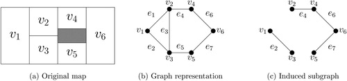
Figure 1(a) presents the running example used throughout this section to illustrate our methodology. In this hypothetical state, we have a total of six precincts, represented as vertices $\{v_1,v_2,\dots ,v_6\}$, which we hope to divide into two districts, $\{V_1,V_2\}$. A gray area is uninhabited (e.g., lake). This map can be represented as a graph of Figure 1(b) where two contiguous vertices share an edge. Consider a redistricting map with $V_1=\{v_1,v_3\}$ and $V_2=\{v_2,v_4,v_5,v_6\}$. As shown in Figure 1(c), this redistricting map can be represented by an induced subgraph after removing three edges, that is, $\{e_1,e_3,e_5\}$. Thus, we can represent each district as an induced subgraph, which is a set of edges, that is, $S(V_1)=\left\{e_2\right\}$ or $S(V_2)=\{e_4,e_6,e_7\}$.

Fig. 1 A running redistricting example. We consider dividing a state with six geographical units into two districts. The original map is shown in the left panel where the shaded area is uninhabited. The middle panel shows its graph representation, whereas the right panel shows an example of redistricting map represented by an induced subgraph, which consists of a subset of edges.

2.2 Graph Partitions and Zero-Suppressed Binary Decision Diagram (ZDD)

A major challenge for enumerating redistricting maps is memory management because the total number of possible maps increases exponentially. We use the ZDD, which uses a compact data structure to efficiently represent a family of sets (Minato 1993). We first discuss how the ZDD can represent a family of graph partitions before explaining how we construct the ZDD from a given graph.

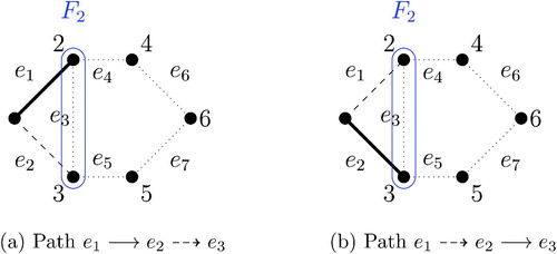
The ZDD that corresponds to the running example of Figure 1 is given in Figure 2. A ZDD is a directed acyclic graph. As is clear from the figure, each edge of the original graph corresponds to possibly multiple nodes of a ZDD. To avoid confusing terminology, we use a “node” rather than a “vertex” to refer to a unit of ZDD, which represents an edge of the original graph. Similarly, we call an edge of the ZDD an “arc” to distinguish it from an edge of the original graph. There are three special nodes in a ZDD. The root node, labeled as e₁ in our example, has no incoming arc but, like other nodes, represents one of the edges in the original graph. We will discuss later how we label nodes. ZDD also has two types of terminal nodes without an outgoing arc, called 0-terminal and 1-terminal nodes and represented by 0 and 1, respectively. Unlike other nodes, these terminal nodes do not correspond to any edge in the original graph. Finally, each nonterminal node, including the root node, has exactly two outgoing arcs, 0-arc (dashed arrow) and 1-arc (solid arrow).

Fig. 2 Zero-suppressed binary decision diagram (ZDD) for the running example of Figure 1(b). The blue path corresponds to the redistricting map represented by the induced subgraph in Figure 1(c).

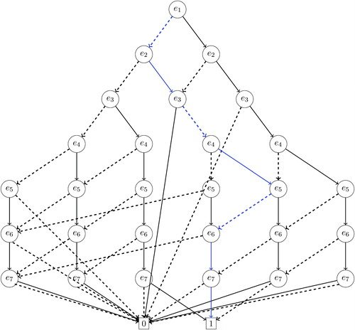
Given a ZDD, we can represent a graph partition as the set of edges that belong to a directed path from the root node to 1-terminal node and have an outgoing 1-arc. For example, the path highlighted by blue, $e_1\mathrm{}-\to e_2\to e_3\mathrm{}-\to e_4\to e_5\mathrm{}-\to e_6\to e_7\to 1$, represents the edge set $\{e_2,e_4,e_6,e_7\}$, which corresponds to the 2-graph partition shown in Figure 1(c). Indeed, there is a one-to-one correspondence between a graph partition and a path of a ZDD.

2.3 Construction of the ZDD

How should we construct a ZDD for a p-graph partition from a given graph? We use the frontier-based search algorithm proposed by Kawahara et al. (2017). The algorithm grows a tree starting with the root node in a specific manner. We first discuss how to construct a ZDD given m labeled edges, $\{e_1,\dots ,e_m\}$, where e₁ represents the root node. We then explain how we merge nodes to reduce the size of the resulting ZDD and how we label edges given a graph to be partitioned so that the computation is efficient.

2.3.1 The Preliminaries

Starting with the root node i = 1, we first create one outgoing 0-arc and one outgoing 1-arc from the corresponding node e_i to the next node $e_{i+1}$. To ensure that each enumerated partitioning has exactly p connected components, we store the number of determined connected components as the dcc variable for each ZDD node. Consider a directed path $e_1\to e_2\mathrm{}-\to e_3\mathrm{}-\to e_4\mathrm{}-\to e_5$. In this example, e₁ is retained whereas edges $\{e_2,e_3,e_4\}$ are not. We know that the two vertices, $\{v_1,v_2\}$, together form one district, regardless of whether or not e₅ is retained. Then, we say that a connected component is determined and set dcc to 1 for e₅. If dcc exceeds p, then we create an arc into the 0-terminal node rather than create an arc into the next node since there is no longer a prospect of constructing a valid partition. Similarly, when creating an arc out of the final node, e_m, we point the arc into the 0-terminal node if dcc is less than p, which represents the total number of partitions. Finally, if the number of remaining edges exceeds $p-\mathit{dcc}$, we stop growing the path by creating an outgoing arc into the 0-terminal node.

How do we find out when another connected component is determined so that $\mathit{dcc}$ needs to be increased? To do this, we need two new variables. First, for each vertex v_i, we store the connected component number, denoted by $\mathit{comp}[v_i]$, indicating the connected component to which v_i belongs. Thus, two vertices, v_i and $v_{i\prime }$, share an identical connected component number if and only if they belong to the same connected component, that is, $\mathit{comp}[v_i]=\mathit{comp}[v_{i\prime }]$.

We initialize the connected component number as $\mathit{comp}[v_i]\leftarrow i$ for $i=1,2,\dots ,n$ where n is the number of vertices in the original graph. Suppose that we process and retain an edge incident to two vertices v_i and $v_{i\prime }$ for $i\ne i\prime$ by creating an outgoing 1-arc. Then, we set $\mathit{comp}[v_j]\leftarrow \max \{\mathit{comp}[v_i],\mathit{comp}[v_{i\prime }]\}$ for any vertex v_j whose current connected component number is given by $\mathit{comp}[v_j]=\min \{\mathit{comp}[v_i],\mathit{comp}[v_{i\prime }]\}$. This operation ensures that all vertices that are connected to v_i or $v_{i\prime }$ have the same connected component number (larger of the two original numbers).

2.3.2 The Frontier-Based Search

Next, we define the frontier of a graph, which changes as we process each edge and grow a tree. Suppose that we have created a directed path by processing the nodes from e₁ up to $e_{\mathcal{l}}$ where $\mathcal{l}=2,3,\dots ,m-1$. For each $\mathcal{l}=1,2,\dots ,m-1$, the $\mathcal{l}$th frontier $F_{\mathcal{l}}$ represents the set of vertices of the original graph that are incident to both a processed edge (i.e., at least one of $e_1,e_2,\dots ,e_{\mathcal{l}}$) and an unprocessed edge (i.e., at least one of $e_{\mathcal{l}+1},e_{\mathcal{l}+2},\dots ,e_m$). Note that we define $F_0=F_m=\varnothing$ and that the set of processed edges includes the one currently being processed. Thus, for a given graph, the frontier only depends on which edge is being processed but does not hinge on how edges have been or will be processed. That is, the same frontier results for each node regardless of paths.

The frontier can be used to check whether a connected component is determined. Specifically, suppose there exists a vertex v that belongs to the previous frontier but is not part of the current one, that is, $v\in F_{\mathcal{l}-1}$ and $v\notin F_{\mathcal{l}}$. Then, if there is no other vertex in $F_{\mathcal{l}}$ that has the same connected component number as v (i.e., no vertex in $F_{\mathcal{l}}$ is connected to v), there will not be another vertex in subsequent frontiers, that is, $F_{\mathcal{l}+1},\dots ,F_m$, that are connected to v. Thus, under this condition, the connected component $\mathit{comp}[v]$ is determined, and we increment dcc by one.

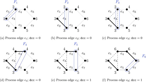
Figure 3 gives an example of computing the connected component number, constructing the frontier, and updating the determined connected components, based on the redistricting problem shown in Figure 1. In each graph, a positive integer placed next to a vertex represents its connected component number, whereas the vertices grouped by the solid line represent a frontier. For example, when processing edge e₅ (see Figure 3(e)), we have $F_4=\{v_3,v_4\}$ and $F_5=\{v_4,v_5\}$. Since there is no vertex in F₅ that shares the same connected component number as v₃ (which is 1), we can determine the first connected component and increment $\mathit{dcc}$ by one.

Fig. 3 Calculation of the frontier, the connected component number, and the determined connected components. This illustrative example is based on the redistricting problem shown in Figure 1. A positive integer placed next to each vertex represents the connected component number, whereas the vertices grouped by the solid blue line represent a frontier. A connected component is determined when processing edge e₅.

Finally, when processing the last edge e_m represented by node $n^{\ast }$, if two vertices incident to the edge belong to the same connected component number, then the 0-arc from node $n^{\ast }$ points to the 0-terminal node whereas the destination of the 1-arc is the 1-terminal node unless dcc $\ne p$. If they have different connected component numbers, the 0-arc of node $n^{\ast }$ goes to the 1-terminal node whereas the destination of its 1-arc is the 1-terminal node so long as dcc $=p$ and the induced subgraph condition described in the next paragraph is satisfied (otherwise, it is the 0-terminal node).

Throughout the process of building a ZDD, we must make sure that every path actually corresponds to an induced subgraph, which is defined as a subset of nodes and all arcs connecting pairs of such nodes. We call this the induced subgraph condition. Consider a path, $e_1\to e_2\to e_3$. Since three vertices, $\{v_1,v_2,v_3\}$, are connected, we must retain edge e₃ because its two incident vertices, v₂ and v₃, are connected. Thus, we have $e_1\to e_2\to e_3\mathrm{}-\to 0$. Similarly, consider a path, $e_1\to e_2\mathrm{}-\to e_3$. We cannot retain e₃ because e₂, which is incident to v₁ and v₃, is not retained. This yields $e_1\to e_2\mathrm{}-\to e_3\to 0$.

To impose the induced subgraph condition, we introduce the forbidden pair set for each node. Once we decide not to use an edge that connects two distinct components, the two components must not be connected any more. Otherwise, the new component generated by connecting the two components has an unused edge, violating the induced subgraph condition. Therefore, if we determine that an edge $\{v,v\prime \}$ is not used, the addition of $\{\mathit{comp}[v],\mathit{comp}[v\prime ]\}$ to the forbidden pair set reminds us that the components $\mathit{comp}[v]$ and $\mathit{comp}[v\prime ]$ must not be connected. That is, if we use an edge $\{u,u\prime \}$ and the forbidden pair set contains $\{\mathit{comp}[u],\mathit{comp}[u\prime ]\}$, the path will be sent to the 0-terminal. In the above example, if we pass through $e_1\to e_2\mathrm{}-\to e_3$, {2, 3} is added to the forbidden pair set, where 2 is the component number of $\{v_1,v_2\}$ and 3 is that of $\left\{v_3\right\}$. Then, since retaining e₃ violates the induced subgraph condition, we have $e_1\to e_2\mathrm{}-\to e_3\to 0$.

2.3.3 Node Merge

The above operation implies that when processing $e_{\mathcal{l}}$, the only required information is the connectivity of vertices in $F_{\mathcal{l}-1}$. We can reduce the size of the ZDD by exploiting this fact. First, we can avoid repeating the same computation by merging multiple nodes if the connected component numbers of all vertices in $F_{\mathcal{l}-1}$ and the number of determined connected components $\mathit{dcc}$ are identical. This is a key property of the ZDD, which allows us to efficiently enumerate all possible redistricting plans by merging many different paths. Second, we only need to examine the connectivity of vertices within a frontier to decide whether or not any connected component is determined. Thus, we adjust the connected component number so that it equals the maximum vertex number in the frontier. That is, if some vertices in the frontier share the same connected component number, we change it to the maximum vertex index among those vertices. For example, in Figure 3(b), we set $\mathit{comp}[v_2]=2$ and $\mathit{comp}[v_3]=3$. We need not worry about how the renumbering of $\mathit{comp}[v_3]$ affects the value of $\mathit{comp}[v_1]$ because $v_1\notin F_2$. This operation results in merging of additional nodes, reducing the overall size of the ZDD.

Figure 4 gives an example of such a merge. Figure 4(a) corresponds to the path, $e_1\to e_2\mathrm{}-\to e_3$ whereas Figure 4(b) represents the path, $e_1\mathrm{}-\to e_2\to e_3$. As shown in Figure 2, these two paths are merged at e₃ because the connected component numbers in their frontier F₂ are identical and both have the same number of determined connected component, that is, $\mathit{dcc}=0$. Note that in Figure 4(b) the connected component number is normalized within the frontier F₂ such that the connected component number of v₂ is the maximum vertex index, that is, 2, and that of v₃ is 3.

Fig. 4 An example of node merging. as shown in Figure 2, these two paths merge at e₃ because the connected component numbers in F₂ are identical and the number of determined connected components is zero.

Node merging plays a key role in scaling up the enumeration algorithm. Although we can construct the ZDD that only enumerates graph partitions by storing the sum of population values into each node (see Kawahara et al. 2017, sec. 4), this prevents nodes from being merged, dramatically reducing the scalability of the enumeration algorithm. Therefore, we do not take this approach here.

2.3.4 Edge Ordering

How should we label the edges of the original graph? The amount of computation depends on the number of nodes in the ZDD. Recall that two nodes are merged if the stored values such as comp and dcc are identical. Since a ZDD node stores the comp value for each vertex in the frontier, the number of unique stored values grows exponentially as the frontier size increases (see Section 3.1 in Kawahara et al. (2017) for the detailed analysis). Therefore, we wish to label the edges of a graph such that the maximum size of the frontier is minimized. We take a heuristic approach here. Specifically, we first choose two vertices s, t such that the shortest distance between s and t is as large as possible across all vertex pairs. We use the Floyd–Warshall algorithm, which can find the shortest paths between all vertex pairs in $\mathcal{O}(|V{|}^3)$ where $\left|V\right|$ is the number of vertices of a graph. Next, we compute the minimum s–t vertex graph cut, which is the minimum set of vertices whose removal generates two or more connected components. To do this, we use a max-flow based algorithm, and arbitrarily order the resulting connected components. Finally, we recursively apply this procedure to each connected component until the resulting connected components are sufficiently small (e.g., 5 edges), at which point they are ordered in an arbitrary fashion.

Figure 5 illustrates this process. In this example, a pair, s = v₁ and t = v₆, gives the maximum shortest distance. Given this choice, there are four minimum s–t graph cuts whose size is 2, that is, $\{v_2,v_3\},\{v_2,v_5\},\{v_3,v_4\},\{v_4,v_5\}$. We arbitrarily select one of them and call it S. Suppose we set $S=\{v_4,v_5\}$. Then, this yields two connected components, that is, $C_1=\{v_1,v_2,v_3\}$ and $C_2=\left\{v_6\right\}$. For each connected component C_i, let E_i represent the set of edges in C_i and between C_i and S. In the current example, $E_1=\left\{\right\{v_1,v_2\},\{v_1,v_3\},\{v_2,v_3\},\{v_2,v_4\},\{v_3,v_5\left\}\right\}$ and $E_2=\left\{\right\{v_4,v_6\},\{v_5,v_7\left\}\right\}$. We order these edge sets so that all the edges E₁ will be placed before those of E₂. To continue this process recursively, we combine all the vertices in S into a single vertex and let this new vertex be t in E₁ and s in E₂. Now, we can apply the same procedure separately to E₁ and E₂: computing the minimum s–t vertex cut and splitting the graph into two (or more) components.

Fig. 5 An example of edge ordering by vertex cuts. To order edges, we choose two vertices with the maximum shortest distance and call them s and t. We then use the minimum vertex cut, indicated by the dashed oval, to create two or more connected components, which are arbitrarily ordered. The same procedure is then applied to each connected component until the resulting connected components are sufficiently small.

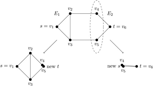
The reason why we expect the above edge ordering procedure to produce a small frontier is that each vertex cut in the process equals one of the frontiers of the corresponding ZDD. In our example, the first vertex cut S is equal to $F_5=\{v_4,v_5\}$. Since we choose minimum vertex cuts in each step, we expect the input graph with the edge order obtained through this procedure to have small frontiers.

2.4 Enumeration and Independent Sampling

It can be shown that every path from the root node to the 1-terminal node in the resulting ZDD has a one-to-one correspondence to a p-graph partition. This is because each p-graph partition can be uniquely represented by the union of induced subgraphs, which in turn corresponds to a unique path from the root node to the 1-terminal node. The complexity of the enumpart algorithm is generally difficult to characterize, but Kawahara et al. (2017) analyzed it in the case of planar graphs. Thus, once we obtain the ZDD as described above, we can quickly enumerate all the paths from the root node to the 1-terminal node. Specifically, we start with the 1-terminal node and then proceed upward to the root node, yielding a unique graph partition.

In addition to enumeration, we can also independently sample p-graph partitions (Knuth 2011). First, for each node ν of the ZDD, we compute the number of paths to the 1-terminal node. Let $c(\nu )$ be the number of such paths, and ν₀ and ν₁ be the nodes pointed by the 0-arc and 1-arc of ν, respectively. Clearly, we have $c(\nu )=c({\nu }_0)+c({\nu }_1)$. The values of c for the 0-terminal and 1-terminal nodes are 0 and 1, respectively. As done for enumeration, we compute and store the value of c for each node by moving upward from the terminal node to the root node. Finally, we conduct random sampling by starting with the root node and choosing node ν₁ with probability $c({\nu }_1)/\{c({\nu }_0)+c({\nu }_1)\}$ until we reach the 1-terminal node. Since the probability of reaching the 0-terminal node is zero, we will always arrive at the 1-terminal node, implying that we obtain a path corresponding to a p-graph partition. Repeating this procedure will yield the desired number of independently and uniformly sampled p-graph partitions.

The reason why this procedure samples redistricting maps uniformly is that a path from the root node to the 1-terminal node corresponds to a unique p-graph partition. Since each node ν stores the number of paths from the node to the 1-terminal node as $c(\nu )$, the sampling procedure uniformly and randomly selects one path among $c(v_1)$ paths where v₁ is the root node. If nonuniform sampling is desired, one could apply the sampling-importance resampling algorithm to obtain a representative sample from a target distribution (Rubin 1987).

3 Empirical Scalability Analysis

This section analyzes the scalability of the enumpart algorithm described above, and shows that the algorithm scales to enumerate partitions of maps many times larger than existing enumeration procedures. We analyze the algorithm’s scalability in terms of runtime and memory usage, and show how the memory usage of enumpart is closely tied to the frontier of the corresponding ZDD as explained in the previous section.

To make this empirical analysis realistic, we use independently constructed and contiguous subsets of the 2008 New Hampshire precinct map for maps ranging between 40 precincts and 200 precincts, increasing by 40, that is, $\{40,80,120,160,200\}$. The original New Hampshire map consists of 327 precincts, which are divided into two congressional districts. To generate an independent contiguous subset of the map, we first randomly sample a precinct, and add its adjacent precincts to a queue. We then repeatedly sample additional precincts from the queue to be added to the subset map, and add the neighbors of the sampled precincts to the queue, until the map reaches the specified size. We repeat this process until the subsetted map reaches a prespecified size.

We consider partitioning each of these maps into two, five, or ten districts and apply enumpart to each case. We then compute the time and memory usage of generating a ZDD for each application. For each precinct size and number of districts, we repeat the above sampling procedure 25 times, producing 25 independent and contiguous subsets of the New Hampshire map. All trials were run on a Linux computing cluster with 530 nodes and 48 Intel Cascade Lake cores per node, where each node has 180GB of RAM. Note that we do not save the results of enumeration to disk as doing so for every trial is computationally too expensive. This means that we cannot conduct an in-depth analysis of the characteristics of all enumerated maps.

Figure 6 shows the results of our scalability analysis. The top row shows scalability results for generating a ZDD for partitions of the map into two districts, while the middle row shows the results with five districts and the bottom row shows results with ten districts. Each dot represents a run of the enumpart algorithm on a subset of the New Hampshire map. Crosses represent trials where the ZDD successfully built using under the 180GB RAM limit. In contrast, open circles show trials that were unable to build the ZDD with the same RAM limit. Note that for the left and middle columns, the results are jittered horizontally with a width of 20 for the clarity of presentation.

Fig. 6 The scalability of the enumpart algorithm on subsets of the New Hampshire precinct map. This figure shows the runtime scalability of the enumpart algorithm for building the ZDD on random contiguous subsets of the New Hampshire precinct map. Crosses indicate maps where the ZDD was successfully built within the RAM limit of 180GB. In contrast, open circles represent maps where the algorithm ran out of memory. For the left and middle columns, the results are jittered horizontally with a width of 20 for the clarity of presentation. (The actual evaluation points on the horizontal axis are 40, 80, 120, 160, and 200.) The left column shows how total runtime increases with the number of units in the underlying map, while the center column shows how the total RAM usage increases with the number of units in the underlying map. Lastly, the right-hand column shows that memory usage is primarily a function of the maximum frontier size of the ZDD. We show results for 2-district partitions (top row), five-district partitions (middle row), and 10-district partitions (bottom row).

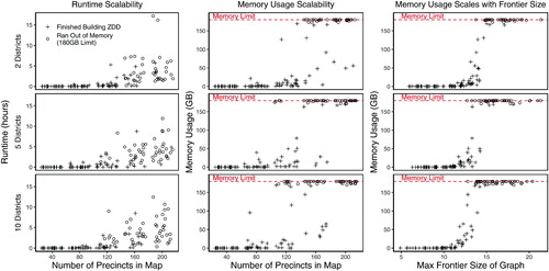
The left-hand and center columns show how the enumpart algorithm scales in terms of runtime and memory usage, respectively, as the number of precincts in the underlying map increases. For small maps ranging from 25 precincts to 80 precincts, runtime and memory usage are for the most part negligible. The ZDD for two-district, five-district, and ten-district partitions for these small maps can be constructed in nearly all cases in under two minutes, and using less than one gigabyte of RAM. As the number of precincts in the map starts to increase, so do the runtime and memory usage requirements. For maps of 200 precincts, over 90% of the tested maps hit the 180GB memory limit before building the complete ZDD. For all map sizes, we also note that the runtime and memory usage requirements for building the ZDD do not appear to depend much on the number of districts that the map is being partitioned into.

What drives these patterns in scalability? While the number of units in the underlying map predicts both runtime and memory usage, there is still a great deal of variability even conditional on the number of precincts in the map. In the right-hand column, we show that the memory usage requirements for building the ZDD are closely tied to the maximum frontier size of the underlying map, as defined in Section 2.3.2. While the memory usage is minimal so long as the maximum frontier size of the graph is under 11, memory usage increases quickly once the maximum frontier size grows beyond that. This suggests that improved routines for reducing the size of a map’s frontier can allow for the enumeration of increasingly large maps.

4 Empirical Validation Studies

In this section, we introduce a set of new validation tests and datasets that can be used to evaluate the performance of redistricting simulation methods. We focus on the two most popular types of simulation methods that are implemented as part of the open-source software package redist (Fifield, Tarr, and Imai 2015): one based on the MCMC algorithm (Fifield et al. 2014; Fifield, Higgins, et al. 2020; Mattingly and Vaughn 2014) and the other based on the RSG algorithm (Cirincione, Darling, and O’Rourke 2000; Chen and Rodden 2013). Below, we conduct empirical validation studies both through full enumeration and independent sampling. For the sake of simplicity, we use the uniform distribution over all valid redistricting maps under various constraints. However, one could also use a nonuniform target distribution by appropriately weighting each map.

4.1 Validation Through Enumeration

We conduct two types of validation tests using enumeration. We first use the enumpart algorithm to enumerate all possible redistricting plans using a map with 70 precincts, which is much larger than the existing validation map with 25 precincts analyzed in Fifield et al. (2014) and Fifield, Higgins, et al. (2020). We then compare the sampled redistricting plans obtained from simulation methods against the ground truth based on the enumerated plans. The second approach is based on many smaller maps with 25 precincts. We then assess the overall performance of simulation methods across these many maps rather than focusing on a specific map.

4.1.1 A New 70-Precinct Validation Map

The top left plot of Figure 7 introduces a new validation map with 70 precincts and their population, which is a subset of the 2008 Florida precinct map consisting of 6,688 precincts with 25 districts. We use the enumpart algorithm to enumerate every partition of this map into two districts, which took approximately 8 hr on a MacBook Pro laptop with 16GB RAM and 2.8 GHz Intel i7 processors. Nearly all of this time was spent writing the partitions to disk—building the ZDD for this map took under half a second.

Fig. 7 A new 70-precinct validation map and the histogram of redistricting plans under various population parity and compactness constraints. The underlying data is a 70-precinct contiguous subset of the Florida precinct map, for which the enumpart algorithm enumerated every 44,082,156 partitions of the map into two contiguous districts. In the histograms, each bar represents the number of redistricting plans that fall within a 1 percentage point range of a certain population parity, that is, $[0,0.01),[0.01,0.02),\dots ,[0.19,0.20)$. The 25th (75th) percentile compactness constraint is defined as the set of plans that are more compact than the 25th (75th) percentile of maps within the full enumeration of all plans for the 70-precinct map, using the Relative Proximity Index to measure compactness. The annotations reflect the exact number of plans which meet the constraints. For example, when no compactness constraint is applied, there are 3,678,453 valid plans when applying a 5% population parity constraint, and 717,060 valid plans when applying a 1% population parity constraint. Under the strictest constraints, the 1% population parity constraint and 75th percentile compactness constraint, there are 271,240 valid plans.

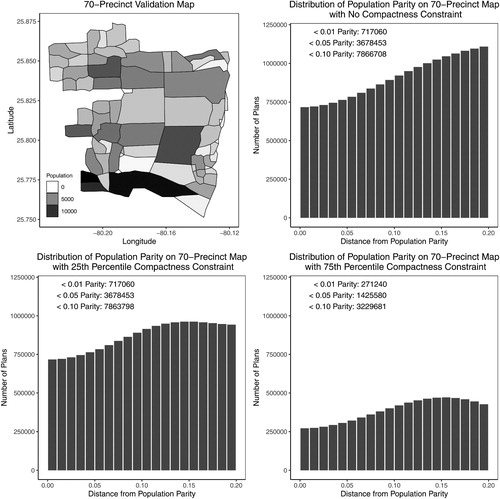
The histograms of the figure shows the number of redistricting plans that satisfy the deviation from population parity up to 20 percentage points (by one percentage point increments, i.e., $[0,0.01),[0.01,0.02),\dots ,[0.19,0.2)$). The deviation from population parity is defined as,(1) $$\underset{{}_{1\le k\le p}}{\max }\frac{|P_k-\overline{P}|}{\overline{P}},$$(1) where P_k represents the population of the kth district, $\overline{P}={\sum }_{k=1}^p{P}_k/p$, and p is the total number of districts. When partitioning this map into two districts, there exist a total of 44,082,156 possible redistricting plans if we only impose the contiguity requirement.

As shown in the upper right plot, out of these, over 700,000 plans are within a 1% population parity constraint. As we relax the population parity constraint, the cumulative number of valid redistricting plans gradually increases, reaching over 3 and 7 million plans for the 5% and 10% population parity constraints, respectively. Thus, this validation map represents a more realistic redistricting problem than the validation map analyzed in Fifield et al. (2014) and Fifield, Higgins, et al. (2020). That dataset, which enumerates all 117,688 partitions of a 25-precinct subset of the Florida map into three districts, includes only 8 plans within 1% of population parity, and 927 plans within 10% of population parity.

In addition to the population parity, we also consider compactness constraints. Although there exist a large number of different compactness measures, for the sake of illustration, we use the relative proximity index (RPI) proposed by Fryer and Holden (2011). The RPI for a given plan π_s in the valid set of redistricting plans $\mathit{\pi }$ is defined as,(2) $$\text{RPI}({\pi }_s)=\frac{\sum _{k=1}^p\sum _{i\in V_k}\sum _{j\in V_k}{P}_i{P}_j{D}_{ij}^2}{\text{arg}{\text{min}}_{{\pi }_s\in \mathit{\pi }}\sum _{k=1}^p\sum _{i\in V_k}\sum _{j\in V_k}{P}_i{P}_j{D}_{ij}^2},$$(2) where P_i corresponds to the population for precinct i assigned to district k, and D_ij corresponds to the distance between precincts i and j assigned to district k. Thus, a plan with a lower RPI is more compact.

We consider two compactness thresholds based on the RPI values: 25th and 75th percentiles, which equal 1.76 and 1.44, respectively. As shown in the bottom left histogram of Figure 7, the 25th percentile constraint does little beyond the population constraint. The number of valid plans that satisfy a 5% population parity threshold remains identical even after imposing this compactness constraint. However, the 75th percentile compactness constraint dramatically reduces the number of valid plans as seen in the bottom right histogram. For example, it reduces the total number of plans that meet the 1% population parity threshold by more than 70%.

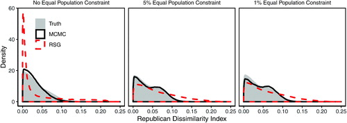
Figure 8 shows the performance of the MCMC and RSG simulation methods using the new 70-precinct validation map (see Algorithms 1 and 3 of Fifield et al. (2014) and Fifield, Higgins, et al. (2020), respectively, for the details of implementation). The solid gray density shows the true distribution of the Republican dissimilarity index (Massey and Denton 1988) on the validation map, which is defined as(3) $$D=\frac{1}{2}\sum _{k=1}^p\frac{P_k}{P}·\frac{|R_k-R|}{R(1-R)},$$(3) where k indexes districts in a state, P_k is the population of district k, R_k is the share of district k that voted for the Republican presidential candidate in 2008, P is the total population in the state, and R is the voteshare for the Republican presidential candidate across all districts.

Fig. 8 A validation study enumerating all partitions of a 70-precinct map into two districts. The underlying data are the 70-precinct contiguous subset introduced in the left plot of Figure 7. Unlike the random-seed-and-grow (RSG) method (red dashed lines), the Markov chain Monte Carlo (MCMC) method (solid black line) is able to approximate the target distribution. The 25th percentile (75th percentile) compactness constraint is defined as the set of plans that are more compact than the 25th (75th) percentile of maps within the full enumeration of all plans for the 70-precinct map, using the Relative Proximity Index to measure compactness.

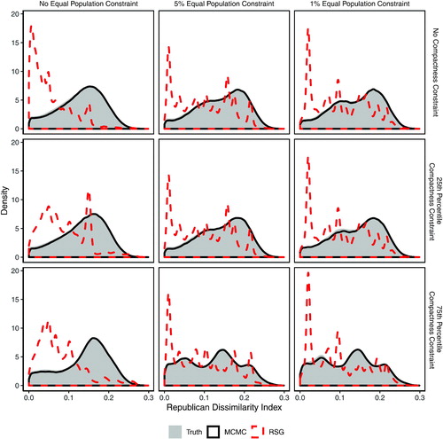
The red dashed lines show the distribution of the Republican dissimilarity index of the RSG algorithm. Solid black lines show the distribution of the Republican dissimilarity index on plans drawn by the MCMC algorithm. In cases where we impose a population parity target, we specify a target distribution of plans using the Gibbs distribution where plans closer to population parity are more likely to be sampled by the algorithm (see Fifield et al. 2014; Fifield, Higgins, et al. 2020, for details).

Similarly, when a compactness constraint is imposed, we specify a target Gibbs distribution such that more compact plans are sampled. Note that in typical redistricting applications, we would not know the denominator of Equation (2)(2) $$\text{RPI}({\pi }_s)=\frac{\sum _{k=1}^p\sum _{i\in V_k}\sum _{j\in V_k}{P}_i{P}_j{D}_{ij}^2}{\text{arg}{\text{min}}_{{\pi }_s\in \mathit{\pi }}\sum _{k=1}^p\sum _{i\in V_k}\sum _{j\in V_k}{P}_i{P}_j{D}_{ij}^2},$$(2) . Fryer and Holden (2011) derived a power-diagram approach to finding a plan that approximately minimizes the denominator. Since we have enumerated all possible plans in the current setting, we simply use the true minimum value. However, this has no impact on the performance of the algorithm, since it is absorbed into the normalizing constant of the target distribution.

Specifically, we use the following target Gibbs distribution,(4) $$f_{\beta }({\pi }_s)=\frac{1}{z(\beta )}\text{exp}\hspace{0.17em}\left\{-\sum _{k=1}^p({\beta }_p{\psi }_k^p+{\beta }_c{\psi }_k^c)\right\},$$(4) where$$\begin{array}{c}{\psi }_k^p=\frac{|P_k-\overline{P}|}{\overline{P}}\hspace{1em}\text{and}\\ {\psi }_k^c=\frac{\sum _{i\in V_k}\sum _{j\in V_k}{P}_i{P}_j{D}_{ij}^2}{\text{arg}{\text{min}}_{{\pi }_s\in \mathit{\pi }}\sum _{k=1}^p\sum _{i\in V_k}\sum _{j\in V_k}{P}_i{P}_j{D}_{ij}^2}.\end{array}$$

In this formulation, the strength of each constraint is governed by separate temperature parameters β_p (for population parity) and β_c (for compactness), where higher temperatures increase the likelihood that plans closer to the population parity or compactness target will be sampled. Once the algorithm is run, we discard sampled plans that fail to meet the target population and compactness constraints, and then reweight and resample the remaining plans so that they approximate a uniform sample from the population of all plans satisfying the constraints. After some initial tuning, we selected ${\beta }_p=10$ for the 5% equal population constraint, and ${\beta }_p=50$ for the 1% equal population constraint. We selected ${\beta }_c=0.001$ for the 25th percentile compactness constraint and ${\beta }_c=0.01$ for the 75th percentile compactness constraint. When the population or compactness constraints are not applied, we set their corresponding temperature parameter to 0.

The RSG algorithm was run for 1,000,000 independent draws for each population constraint, while the MCMC algorithms were run for 250,000 iterations using 8 chains for each pair of constraints. Starting plans for each MCMC chain were independently selected using the RSG algorithm. The Gelman–Rubin diagnostic (Gelman and Rubin 1992), a standard diagnostic tool for MCMC methods based on multiple chains, suggests that all MCMC chains had converged after at most 30,000 iterations. Unfortunately, the RSG algorithm does not come with such a diagnostic and hence we simply run it until it yields the same number of draws as the MCMC algorithms for the sake of comparison.

It is clear that on this test map, the RSG algorithm is unable to obtain a representative sample of the target distribution, at any level of population parity or compactness. This finding is consistent with the fact that the RSG algorithm is a heuristic algorithm with no theoretical guarantees and no specified target distribution. In contrast, the MCMC algorithm is able to approximate the target distribution, across all levels of population parity and compactness tested.

4.1.2 Many Small Validation Maps

A potential criticism of the previous validation study is that it is based on a single map. This means that even though it is of much larger size than the previously available validation map, the results may depend on the idiosyncratic geographical and other features of this particular validation map. To address this, we conduct another study based on many small validation maps. Specifically, we use our algorithm to enumerate all possible redistricting plans for each of 200 independent 25-precinct subsets of the 2008 Florida map. We then evaluate the performance of simulation methods for each validation map. Since we do not tune the temperature parameter of the MCMC algorithm for each simulated map unlike what one would do in practice, this yields a simulation setting that poses a significant challenge for the MCMC algorithm.

To assess the overall performance across these validation maps, we use the Kolmogorov–Smirnov (KS) statistic to test the distributional equality of the Republican dissimilarity index between the enumerated plans and the simulated plans. To increase the independence across simulated plans, we run the MCMC and RSG algorithms for 5 million iterations each on every map and then thinning by 500 (i.e., taking every 500th posterior draw). Without thinning, there is a significant amount of autocorrelation across draws, with the autocorrelation typically ranging between 0.75 and 0.85 between adjacent draws and between 0.30 and 0.60 for draws separated by 5 iterations. In contrast, when thinning the Markov chain by 500, the autocorrelation between adjacent draws falls to under 0.05. When thinning the Markov chain by 1000, the results are approximately the same, as seen in Figure A.1.

Although this does not make simulated draws completely independent of one another, we compute the p-value under the assumption of two independently and identically distributed samples. If the simulation methods are successful and the independence assumption holds, then we should find that the distribution of p-values across 200 small validation maps should be approximately uniform. After some initial tuning, we set the temperature parameter of the MCMC algorithm such that ${\beta }_p=1$ for the 20% equal population constraint, and ${\beta }_p=5$ for the 10% equal population constraint. These values are used throughout the simulations. After running the simulations, we again discard plans falling outside of the specified parity threshold and then reweight and resample the remaining plans to approximate a uniform draw from the target distribution of plans satisfying the specified parity constraint. We then calculate the KS test p-value by comparing the reweighted and resampled set of plans against the true distribution.

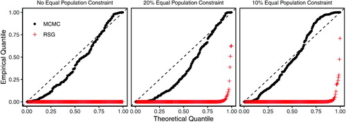
Figure 9 shows the results of this validation study. The left plot shows how the MCMC (black dots) and RSG (red crosses) algorithms perform when not applying any population parity constraint. Each dot corresponds to the p-value of the KS test for a separate 25-precinct map. Under the assumption of independent sampled plans, if a simulation algorithm is successfully approximating the target distribution, these dots should fall roughly on the 45 degree line.

Fig. 9 Quantile-quantile plot of p-values based on the Kolmogorov–Smirnov (KS) tests of distributional equality between the enumerated and simulated plans across 200 validation maps and under different population parity constraints. Each dot represents the p-value from a KS test comparing the empirical distribution of the Republican dissimilarity index from the simulated and enumerated redistricting plans. Under independent and uniform sampling, we expect the dots to fall on the 45 degree line. The MCMC algorithm (black dots), although imperfect, significantly outperforms the RSG algorithm (red crosses). See Figure A.1 in the appendix for discussion of thinning values.

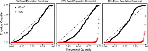
It is clear from this validation test that the RSG algorithm consistently fails to obtain a representative sample of the target distribution. That the red dots are concentrated near the bottom of the graph indicates that the KS p-value for the RSG algorithm is near zero for nearly every map tested. When population parity constraints of 20% and 10% are applied, the RSG algorithm continues to perform poorly compared to the MCMC algorithm. By using a soft constraint based on the Gibbs distribution, we allow the Markov chain to traverse from one valid plan to another through intermediate plans that may not satisfy the desired parity constraint. We find that although imperfect, the MCMC algorithm works much better than RSG algorithm.

4.2 Validation Through Independent Sampling

Next, we conduct larger-scale validation studies by leveraging the fact that the enumpart algorithm can independently sample from the population of all possible redistricting plans. This feature allows us to scale up our validation studies further by avoiding for larger maps the computationally intensive task of writing to the hard disk all possible redistricting plans, which exponentially increases as the map size gets larger or as we try to partition a map into more districts. We independently sample a large number of redistricting plans and compare them against the samples obtained from simulation methods. Below, we present two validation studies. The first study uses the actual Congressional district maps from Iowa, where by law redistricting is done using 99 counties. The second study is based on a new 250-precinct validation map obtained from the Florida map.

4.2.1 The Iowa Congressional District Map

We first analyze a new validation dataset constructed on the redistricting map from the state of Iowa. In Iowa, redistricting is conducted using a total of 99 counties instead of census blocks to piece together districts, to avoid splitting county boundaries in line with the Iowa State Constitution.⁷ As a result, the Iowa redistricting problem is more manageable than other states.

The left plot of Figure 10 shows the Iowa map, where the shading indicates the population of each county. In 2016, Republicans won three districts while Democrats won one district, while in 2018, Democrats won three districts and the Republicans held only one. We use the enumpart algorithm to independently and uniformly sample 500 million contiguous partitions of this map into four districts. This number is minuscule relative to the total number of valid partitions of the map into four districts, of which there are approximately 10²⁴, but still is more than enough to use it as the target distribution. We note that while it took around 36 hr to sample 500 million partitions on the aforementioned computer cluster using significant parallelization, building the ZDD for this map took less than half a second on our MacBook Pro laptop mentioned earlier. Nearly all of the runtime of the enumeration was spent writing the solutions to harddisk.

Fig. 10 Iowa’s 2016 congressional districts and the histogram of a random sample of redistricting plans under various population parity constraints. The underlying data is the Iowa county map, for which the enumpart algorithm generated an independent and uniform random sample of 500 million partitions of the map into four contiguous districts. In the histogram, each bar represents the number of redistricting plans that fall within the 1 percentage point range of a certain population parity, that is, $[0,0.01),[0.01,0.02),\dots ,[0.19,0.20)$. There are 36,131 valid plans when applying a 5% population parity constraint, and only 300 valid plans when applying a 1% population parity constraint.

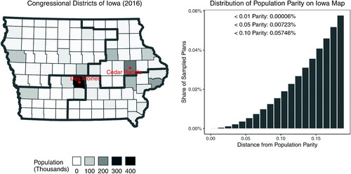
The histogram in Figure 10 shows the share of the sampled redistricting plans that satisfy the deviation from population parity up to 20 percentage points. Of the 500 million plans we have randomly sampled, only 300, or less than 0.00006%, satisfy a 1% population parity constraint, illustrating the sheer scale of the redistricting problem and how much the population equality constraint alone shrinks the total solution space of valid redistricting plans. There are 36,131 plans, or less than 0.001%, satisfying a 5% population parity constraint, which is still a minuscule share compared to the total number of enumerated plans.

Figure 11 shows the performance of the MCMC and RSG simulation methods on the state-sized redistricting problem for Iowa. The solid gray density shows the distribution of the Republican dissimilarity index based on the independently and uniformly sampled set of 500 million redistricting plans. The red dashed lines show the distribution of the Republican dissimilarity index on plans sampled by the RSG algorithm, while the solid black lines shows the distribution for plans sampled by the MCMC algorithm. As in the previous validation exercise, where we impose 5% and 1% population parity constraints, we specify a target distribution of plans using the Gibbs distribution. Here, we set the temperature parameter ${\beta }_p=25$ for the 5% parity constraint, and ${\beta }_p=50$ for the 1% parity constraint, which we selected after initial tuning. After discarding plans not satisfying the constraint and then reweighting, we ended up with 629,729 plans for the 5% parity constraint, and 93,046 plans for the 1% parity constraint. The RSG algorithm was run for 2 million independent draws, while the MCMC algorithms were run for 250,000 iterations and initializing 8 chains for each algorithm. The chains were run without a burn-in period, and the Gelman–Rubin diagnostic suggested that the Markov chains had converged after at most 30,000 iterations.

Fig. 11 A validation study, uniformly sampling from the population of all partitions of the Iowa map into four districts. The underlying data are Iowa’s county map in the left plot of Figure 10, which is partitioned into four congressional districts. As in the previous validation exercises, the Markov chain Monte Carlo (MCMC) method (solid black line) is able to approximate the independently and uniformly sampled target distribution, while the random-seed-and-grow (RSG) method (red dashed line) performs poorly.

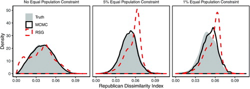
As with the previous validation test, the MCMC algorithm outperforms the RSG algorithm across all levels of the population parity constraint. When no equal population constraint is applied or a 5% population parity constraint is applied, the MCMC algorithm samples from the target distribution nearly perfectly. Even with the 1% parity map, where there are only 300 valid plans in the target distribution, the MCMC algorithm approximates the target distribution reasonably well, missing by only slightly in portions of the distribution. In contrast, at all levels of population parity, the RSG algorithm is unable to draw a representative sample of plans from the target distribution.

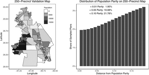
4.2.2 A New 250-Precinct Validation Map

Next, we present the results of validation tests that use a new, 250-precinct validation map, which is constructed from a contiguous subset of the 2008 Florida precinct map. As with the previous validation exercise, we use the enumpart algorithm to independently sample 100 million partitions of this map into two districts. This is still a minuscule number of plans relative to about $5\times {10}^{39}$ possible partitions of this map into two districts. However, given the ability of the enumpart algorithm to independently sample plans using the ZDD, we are able to approximate an accurate target distribution arbitrarily well.

The left plot of Figure 12 shows the validation map, where the shading indicates the population of each of the precincts. Unlike the Iowa map, this map has geographical units of various sizes. This validation map also has a slightly larger frontier size (maximum frontier of 14) than that of the Iowa map (maximum frontier of 11), making it more likely to run out of memory due to the size of ZDD and thereby also increasing computational time. The histogram on the right gives the distribution of population parity distance among the sampled plans, through 20% parity. Of the sampled plans, 1.95% (1.95 million plans) satisfy the 1% population parity constraint, while 21.8% of the sampled plans (21.8 million plans) satisfy the 10% population parity constraint.

Fig. 12 A new 250-precinct validation map and the histogram of redistricting plans under various population parity constraints. The underlying data are a 250-precinct contiguous subset of the Florida precinct map, for which the enumpart algorithm generated an independent and uniform random sample of 100 million partitions of the map into two contiguous districts. In the histogram, each bar represents the number of redistricting plans that fall within the 1 percentage point range of a certain population parity, that is, $[0,0.01),[0.01,0.02),\dots ,[0.19,0.20)$. There are 10,082,542 valid plans when applying a 5% population parity constraint, and 1,953,736 valid plans when applying a 1% population parity constraint.

We sample 4 million plans for each population parity level using the MCMC and RSG algorithms. For the MCMC algorithm, we initialized 8 chains running for 500,000 iterations each, and where a population parity constraint is imposed, we specify the target distribution of plans using the Gibbs distribution. We set the temperature parameter ${\beta }_p=25$ for sampling plans within 5% of parity, and ${\beta }_p=50$ when sampling plans within 1% of parity. After discarding invalid plans and reweighting, these parameter settings yielded 3,088,086 plans satisfying the 5% parity constraint, and 1,881,043 plans satisfying the 1% parity constraint. All 8 chains were run without burn-in, and the Gelman–Rubin convergence diagnostic suggested the chains had converged after approximately 75,000 iterations.

Results for the validation test using the 250-precinct validation map are shown in Figure 13. As with the previous validation exercise, the solid gray density shows the target distribution of the Republican dissimilarity index on the 100 million plans sampled by the enumpart algorithm, while the red dashed lines show the distribution of the Republican dissimilarity index for the RSG algorithm. Finally, the solid black lines show the distribution of the Republican dissimilarity index for the MCMC algorithm. Across all levels of population parity, including the 1% constraint, the MCMC algorithm is able to successfully sample from the target distribution and return a representative sample of redistricting plans. In contrast, where no population parity constraint is applied or where a 5% parity constraint is applied, the RSG algorithm is not able to sample from the target distribution with any accuracy. While it performs somewhat better on the 1% constraint, it is still biased toward plans with higher values on the dissimilarity index, and fails to capture the bimodality of the target distribution.

Fig. 13 A validation study enumerating all partitions of a 250-precinct map into two districts. The underlying data are the 250-precinct contiguous subset introduced in the left plot of Figure 12. As in the previous validation exercises, the Markov chain Monte Carlo (MCMC) method (solid black line) is able to approximate the target distribution based on the independent and uniform sampling, while the random-seed-and-grow (RSG) method (red dashed line) performs poorly.

5 Concluding Remarks

More than a half century after scholars began to consider automated redistricting, legislatures and courts are increasingly relying on computational methods to generate redistricting plans and determine their legality. Unfortunately, despite the growing popularity of simulation methods in the recent redistricting cases, there exists little empirical evidence that these methods can in practice generate a representative sample of all possible redistricting maps under the statutory guidelines and requirements.

We believe that the scientific community has an obligation to empirically validate the accuracy of these methods. In this article, we show how to conduct empirical validation studies by utilizing a recently developed computational method that enables the enumeration and independent sampling of all possible redistricting plans for maps with a couple of hundred geographical units. We make these validation maps publicly available, and implement our methodology as part of an open source software package, redist. These resources should facilitate researchers’ efforts to evaluate the performance of existing and new methods in realistic settings.

Indeed, much work remains to be done to understand the conditions under which a specific simulation method do and does not perform well. A real-world redistricting process is complex. Distinct geographical features and diverse legal requirements play important roles in each state. It is far from clear how these factors interact with different simulation methods. Future work should address these issues using the data from various states.

It is also important to further improve the capabilities of the enumpart algorithm and of the MCMC algorithm. The maximum frontier size of our largest validation maps, which predicts the computational difficulty for the enumpart algorithm, is 14, which is far less than that of other states. For example, the maximum frontier size for New Hampshire (2 districts, 327 precincts) and Wisconsin (8 districts, 6895 precincts) are 21 and 84, respectively. These are much more challenging redistricting problems than the validation studies presented in this article.

As the 2020 census passes, lawsuits challenging proposed redistricting plans will inevitably be brought to court, and simulation evidence will be used to challenge and defend those plans. Thus, it is necessary that the empirical performance of these methods be rigorously evaluated. This article introduces what we hope will be the first of many future complementary validation tests used to ensure that this evidence is of the highest possible quality according to scientific standards.

Supplementary Materials

Replication materials and enumeration results are available as Fifield, Imai, et al. (2020).

Acknowledgments

We thank Steve Schecter, participants of the Quantitative Gerrymandering and Redistricting Conference at Duke University, and two anonymous reviewers for helpful comments.

ORCID

Benjamin Fifield http://orcid.org/0000-0002-2247-0201

Kosuke Imai http://orcid.org/0000-0002-2748-1022

Christopher T. Kenny http://orcid.org/0000-0002-9386-6860

Additional information

Funding

Kawahara acknowledges financial support by JSPS KAKENHI grant number JP18K04610. The computations in this article were run on the FASRC Cannon cluster supported by the FAS Division of Science Research Computing Group at Harvard University.

Appendix

Figure A.1 provides comparison to Figure 9. In Figure 9, thinning for the MCMC runs was set to 500. For this run, thinning for the MCMC runs was set to 1000. We find no significant difference between the two values. Thinning at 500 should then be sufficient and more efficient for this case.

Fig. A.1 Quantile-quantile plot of p-values based on the Kolmogorov–Smirnov (KS) tests of distributional equality between the enumerated and simulated plans across 200 validation maps and under different population parity constraints. Each dot represents the p-value from a KS test comparing the empirical distribution of the Republican dissimilarity index from the simulated and enumerated redistricting plans. Under independent and uniform sampling, we expect the dots to fall on the 45 degree line. The MCMC algorithm (black dots), although imperfect, significantly outperforms the RSG algorithm (red crosses).

References

- Altman, M. (1997), “The Computational Complexity of Automated Redistricting: Is Automation the Answer,” Rutgers Computer & Technology Law Journal, 23, 81–142.
- Altman, M., and McDonald, M. P. (2011), “BARD: Better Automated Redistricting,” Journal of Statistical Software, 42, 1–28. DOI: 10.18637/jss.v042.i04.
- Carter, D., Herschlag, G., Hunter, Z., and Mattingly, J. (2019), “A Merge-Split Proposal for Reversible Monte Carlo Markov Chain Sampling of Redistricting Plans,” Tech. Rep., arXiv no. 1911.01503.
- Chen, J., and Rodden, J. (2013), “Unintentional Gerrymandering: Political Geography and Electoral Bias in Legislatures,” Quarterly Journal of Political Science, 8, 239–269. DOI: 10.1561/100.00012033.
- Chikina, M., Frieze, A., and Pegden, W. (2017), “Assessing Significance in a Markov Chain Without Mixing,” Proceedings of the National Academy of Sciences of the United States of America, 114, 2860–2864. DOI: 10.1073/pnas.1617540114.
- Cirincione, C., Darling, T. A., and O’Rourke, T. G. (2000), “Assessing South Carolina’s 1990s Congressional Districting,” Political Geography, 19, 189–211. DOI: 10.1016/S0962-6298(99)00047-5.
- DeFord, D., Duchin, M., and Solomon, J. (2019), “Recombination: A Family of Markov Chains for Redistricting,” Tech. Rep., arXiv no. 1911.05725.
- Fifield, B., Higgins, M., Imai, K., and Tarr, A. (2014), “A New Automated Redistricting Simulator Using Markov Chain Monte Carlo,” Tech. Rep., Presented at the 31th Annual Meeting of the Society for Political Methodology, University of Georgia.
- Fifield, B., Higgins, M., Imai, K., and Tarr, A. (2020), “Automated Redistricting Simulator Using Markov Chain Monte Carlo,” Journal of Computational and Graphical Statistics (forthcoming).
- Fifield, B., Imai, K., Kawahara, J., and Kenny, C. T. (2020), “Replication Data for: The Essential Role of Empirical Validation in Legislative Redistricting Simulation,” available at https://doi.org/10.7910/DVN/NH4CRS.
- Fifield, B., Tarr, A., and Imai, K. (2015), “redist: Markov Chain Monte Carlo Methods for Redistricting Simulation,” Comprehensive R Archive Network (CRAN), available at https://CRAN.R-project.org/package=redist.
- Fryer, R. G., and Holden, R. (2011), “Measuring the Compactness of Political Districting Plans,” The Journal of Law and Economics, 54, 493–535. DOI: 10.1086/661511.
- Gelman, A., and Rubin, D. B. (1992), “Inference From Iterative Simulations Using Multiple Sequences” (with discussion), Statistical Science, 7, 457–472. DOI: 10.1214/ss/1177011136.
- Herschlag, G., Ravier, R., and Mattingly, J. C. (2017), “Evaluating Partisan Gerrymandering in Wisconsin,” Tech. Rep., Department of Mathematics, Duke University.
- Hess, S. W., Weaver, J. B., Siegfeldt, H. J., Whelan, J. N., and Zitlau, P. A. (1965), “Nonpartisan Political Redistricting by Computer,” Operations Research, 13, 998–1006. DOI: 10.1287/opre.13.6.998.
- Katz, J., King, G., and Rosenblatt, E. (2020), “Theoretical Foundations and Empirical Evaluations of Partisan Fairness in District-Based Democracies,” American Political Science Review, 114, 164–178. DOI: 10.1017/S000305541900056X.
- Kawahara, J., Horiyama, T., Hotta, K., and Minato, S. (2017), “Generating All Patterns of Graph Partitions Within a Disparity Bound,” in Proceedings of the 11th International Conference and Workshops on Algorithms and Computation, Vol. 10167, pp. 119–131.
- Knuth, D. E. (2011), The Art of Computer Programming: Combinatorial Algorithms, Part I (Vol. 4A), New York: Addison-Wesley.
- Liu, Y. Y., Tam Cho, W. K., and Wang, S. (2016), “PEAR: A Massively Parallel Evolutionary Computation Approach for Political Redistricting Optimization and Analysis,” Swarm and Evolutionary Computation, 30, 78–92.
- Magleby, D., and Mosesson, D. (2018), “A New Approach for Developing Neutral Redistricting Plans,” Political Analysis, 26, 147–167. DOI: 10.1017/pan.2017.37.
- Massey, D. S., and Denton, N. A. (1988), “The Dimensions of Residential Segregation,” Social Forces, 67, 281–315. DOI: 10.2307/2579183.
- Mattingly, J. C., and Vaughn, C. (2014), “Redistricting and the Will of the People,” Tech. Rep., Department of Mathematics, Duke University.
- McCarty, N., Poole, K. T., and Rosenthal, H. (2009), “Does Gerrymandering Cause Polarization?,” American Journal of Political Science, 53, 666–680. DOI: 10.1111/j.1540-5907.2009.00393.x.
- Mehrotra, A., Johnson, E., and Nemhauser, G. L. (1998), “An Optimization Based Heuristic for Political Districting,” Management Science, 44, 1100–1114. DOI: 10.1287/mnsc.44.8.1100.
- Minato, S. (1993), “Zero-Suppressed BDDs for Set Manipulation in Combinatorial Problems,” in Proceedings of the 30th ACM/IEEE Design Automation Conference, pp. 272–277.
- Nagel, S. S. (1965), “Simplified Bipartisan Computer Redistricting,” Stanford Law Journal, 17, 863–899. DOI: 10.2307/1226994.
- Rubin, D. B. (1987), “Comment: A Noniterative Sampling/Importance Resampling Alternative to the Data Augmentation Algorithm for Creating a Few Imputation When Fractions of Missing Information Are Modest: The SIR Algorithm,” Journal of the American Statistical Association, 82, 543–546. DOI: 10.2307/2289460.
- Vickrey, W. (1961), “On the Prevention of Gerrymandering,” Political Science Quarterly, 76, 105–110. DOI: 10.2307/2145973.
- Weaver, J. B., and Hess, S. W. (1963), “A Procedure for Nonpartisan Districting: Development of Computer Techniques,” Yale Law Journal, 73, 288–308. DOI: 10.2307/794769.
Appendix
provides comparison to . In , thinning for the MCMC runs was set to 500. For this run, thinning for the MCMC runs was set to 1000. We find no significant difference between the two values. Thinning at 500 should then be sufficient and more efficient for this case.