Quantifying Gerrymandering in North Carolina

ABSTRACT

By comparing a specific redistricting plan to an ensemble of plans, we evaluate whether the plan translates individual votes to election outcomes in an unbiased fashion. Explicitly, we evaluate if a given redistricting plan exhibits extreme statistical properties compared to an ensemble of nonpartisan plans satisfying all legal criteria. Thus, we capture how unbiased redistricting plans interpret individual votes via a state’s geo-political landscape. We generate the ensemble of plans through a Markov chain Monte Carlo algorithm coupled with simulated annealing based on a reference distribution that does not include partisan criteria. Using the ensemble and historical voting data, we create a null hypothesis for various election results, free from partisanship, accounting for the state’s geo-politics. We showcase our methods on two recent congressional districting plans of NC, along with a plan drawn by a bipartisan panel of retired judges. We find the enacted plans are extreme outliers whereas the bipartisan judges’ plan does not give rise to extreme partisan outcomes. Equally important, we illuminate anomalous structures in the plans of interest by developing graphical representations which help identify and understand instances of cracking and packing associated with gerrymandering. These methods were successfully used in recent court cases. Supplementary materials for this article are available online.

KEYWORDS:

• Common Cause v. Rucho
• Gerrymandering
• Monte Carlo sampling
• Redistricting

1 Introduction

In the 2012 NC congressional election, over half the total votes went to Democratic candidates, yet only four of the thirteen elected congressional representatives were Democrats. Furthermore, the most Democratic district had 29.63% margin of victory, whereas the most Republican district had a 13.11% margin of victory. These results may be due to political gerrymandering or, alternatively, be natural outcomes of NC’s geo-political structure as determined by the spatial distribution of partisan votes.

Partisan gerrymandering alters election results away from what would have happened under a “fair” or neutral redistricting process. To detect a gerrymander we must first understand what this baseline is, along with how it may fluctuate. Many existing methods, such as partisan bias and the efficiency gap, assume a baseline of partisan symmetry associated with statewide vote counts. For example, one may be tempted to suppose that the statewide fraction of partisan seats should reflect the statewide fraction of partisan votes; such a relationship would be appropriate under a system based on proportionality, however, we elect representatives under geographically localized districts rather than according to statewide vote fractions.

To understand redistricting in a neutral setting, held under our district-based system of representation, we probe the geo-political structure (i) gathering a collection of redistricting plans that are representative of our sampling procedure which is designed to draw plans that adhere to nonpartisan redistricting criteria; (ii) next, we use historic partisan votes on each of our sampled redistricting plans to understand various plausible voting preferences within each district; and (iii) we aggregate election results to construct the distributions of partisan vote balance on each district and of the congressional delegation’s partisan composition. Districts that are extreme outliers with respect to the ensemble are considered gerrymandered. When a districting plan is gerrymandered, the congressional delegations partisan composition is apt to favor one party over the other compared to what would be predicted among districts developed without partisan criteria. We use a variety of historic elections to obtain plausible partisan preferences within a given district. Such elections include, for example, statewide gubernatorial or presidential races. Each historic election provides a different instrument to probe the structure of a given map: For example, the 2012 presidential and the collection of 2016 congressional races differ in statewide partisan vote fraction, and may also have different spatial voting patterns. For example, sometimes the suburbs vote with the city core and sometimes they do not, depending on the year and contest.

Having probed the impact of the geo-political structure, we analyze three specific districting plans: the two most recent districting plans of NC for the U.S. House of Representatives and a plan proposed by a bipartisan panel of retired NC judges. By situating the election outcomes of these three districting plans in our sampled ensemble, we determine whether the three districting plans contain unlikely partisan favoritism and thwart the underlying geo-political structure, as expressed by the people’s votes, by shifting each district’s partisan vote balance significantly away from what is typical.

An earlier version of this analysis played a central role in Common Cause v. Rucho which was the second federal judgment in the past 30 years that declared a districting plan was a political gerrymander. The case was brought to the U.S. Supreme court, and the analysis was discussed during oral arguments. The Court ultimately decided that partisan gerrymandering was not a matter for the Federal Courts. A North Carolina state court, however, did rule that the congressional districts must be redrawn in Harper v. Lewis and this analysis was used in the remedial process. A related analysis was used to demonstrate racial gerrymandering in Covington v. North Carolina, which caused the courts to intervene in the North Carolina Legislative districts by appointing a special master to redraw some of the districts. Subsequently, a related analysis, also adapted to the North Carolina Legislative, was central in state court case Common Cause v. Lewis which found the N.C. State Legislative maps in violation of the state constitution and resulted in their redrawing. We have also used these techniques to understand gerrymandering in the Wisconsin Legislature (Herschlag, Ravier, and Mattingly 2017) and in Maryland (Lebovici et al. 2018). Our report on Wisconsin was featured in an amicus brief in the US Supreme Court case of Gill v. Whitford (Lander 2017).

The qualitative results and subsequent conclusions of this note agree fully with those in earlier iterations of this analysis reported in Bangia et al. (2017). They also agree in identifying the current maps as outliers with the much more preliminary and simplistic analysis performed in Mattingly and Vaughn (2014) which began the authors’ investigations of these questions.

For elaborations of the ideas presented here and applications to other settings, please see the Quantifying Gerrymandering Blog (Herschlag and Mattingly 2018).

2 Methods

To sample from the space of congressional redistricting plans, we construct a family of probability distributions that are concentrated on plans adhering to non-partisan design criteria from proposed legislation. The non-partisan design criteria ensure that

1. the state population is evenly divided among the thirteen congressional districts,

2. the districts are connected and compact,

3. splitting counties is minimized, and

4. African-American voters are sufficiently concentrated in two districts to affect the winner.

The first three criteria come from House Bill 92 (HB92) of the NC General Assembly, which passed the House during the 2015 legislative session. HB92 also states that a districting plan should comply with the Voting Rights Act (VRA); the fourth criterion aims to ensure that the VRA is satisfied, in line with a redistricting plan proposed by the legislature along with recent court rulings. HB92 proposed establishing a bipartisan redistricting commission guided solely by these principles (see Section S3 of the supplementary materials for the precise criteria). We emphasize that no partisan voting data or demographics were used when sampling redistricting plans.

There is no consensus probability distribution to select compliant redistricting plans. For example, there is no criterion that determines when a plan contains districts that are not compact enough; it is also unclear if a distribution of plans should more heavily weight more compliant plans, or whether it should equally weight all compliant plans. In short, there is no “correct” choice for this distribution, however, we choose distributions that focus the probability on districting plans that adhere to the desired criteria. Our experience to date is that maps that are extreme outliers according to one distribution are also outliers according to alternative distributions. This has been observed now in three court cases where multiple experts used different sampling techniques and distributions but ultimately drew the same conclusion (see LWV 2018; Com 2019a, 2019b). We define a particular score function and use it to define a Gibbs distribution; for our main results, we find compliant plans through a simulated annealing procedure based on this distribution. The score function encapsulates particular legal and societal principles to be considered in redistricting and their relative importance. This is a basic input on which our analysis depends. Details on generating the ensemble of redistricting plans may be found in Section S1 of the supplementary materials.

Based on plans sampled from the sequence of iterative simulation draws after a convergence criterion has been met, we find key results to be qualitatively similar when inputs to the evaluation strategy are perturbed (see Section S5.3 of the supplementary materials). Key findings have also remained stable across different choices of simulated-annealing tuning parameters and different thresholds for assessing compliance with legal requirements such as those governing splits of counties (see Section S5 of the supplementary materials). This provides compelling evidence that our algorithm converges to the fixed distribution associated with our sampling methodology.

Redistricting plans are sampled with a standard Markov chain Monte Carlo algorithm combined with a simulate annealing heating and cooling schedule. About 66,544 random redistricting plans were produced. Additionally, we demonstrated the convergence and robustness of our sampling procedure in Sections S4 and S5 of the supplementary materials). For each generated redistricting plan, we retally the actual historic votes from a variety of electoral races, including the 2012 and 2016 US congressional elections, producing ensembles of election outcomes.

When retallying the votes, we are implicitly making the assumption that people vote for parties rather than people. Although this assumption may not be valid as a precise predictive tool, we do remark (i) averaging past election results was used when drawing maps for partisan advantage and proven to be an effective tool (Com 2019a), and (ii) each election provides a plausible vote structure with which to compare an ensemble with a map of interest. We emphasize that we are not using registration data but the preference expressed though the vote cast in a particular election. In this way, we are capturing some essence of swing and unaffiliated voter preferences at a moment of time. One could insert any model available of precinct-level vote. Investigations in this direction are beyond the scope of the present article. We are less interested in being predictive about what might have happened; but rather, we are using each election vote count as a probe to expose and understand the difference between various maps. We use the ensemble of election outcomes to quantify how extreme a particular districting plan is by observing its place in this collection; we also use the ensemble to quantify gerrymandering by identifying districts that have an atypical partisan concentration of voters.

We analyze and critique three districting plans for the North Carolina’s U.S. Congressional districts:

1. The plan used by North Carolina in 2012, which was subsequently overturned (NC2012);

2. The plan used by North Carolina in 2016, which was recently judged to violate the states constitution (NC2016);

3. A plan developed by a bipartisan group of retired judges as part of the Beyond Gerrymandering project spearheaded by Thomas Ross and the Duke POLIS Center (Tom Ross and POLIS Center at Duke 2016) (Judges).

See Figure S2 in the supplementary materials for the district maps.

Using a related methodology, we assess to what degree three districting plans of interest (NC2012, NC2016, and Judges) are gerrymander when compared to plans with similar spatial structure. This is done by seeing how close each districting plans’ properties are to the collection of nearby redistricting plans. Small changes to district boundaries should not have a significant effect on the character of election results. This analysis is similar, in spirit, to that of Chikina, Frieze, and Pegden (2017).

3 Results

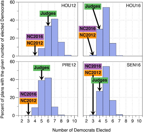
Using our ensemble of 66,544 redistricting plans, we tabulate the observed distribution of the congressional delegation’s partisan composition over a number of historic elections. We situate the NC2012, NC2016, and Judges districting plans on these distributions (see Figure 1 for four of these elections).¹ The partisan composition of the NC2012 and NC2016 districting plans occur in less than 0.3% and 1.1% of our generated redistricting plans for the 2012 and 2016 congressional elections, respectively, and is heavily biased toward the Republicans. When repeating this analysis for the 2012 presidential race and the 2016 United States Senate race, we find that the partisan composition of the NC2012 and NC2016 districting plans occur in less than 0.2% and 0.8% of our generated redistricting plans, respectively. In contrast, the partisan composition of Judges districting plan occurs in 33.5% and 30% of our generated redistricting plans for the 2012 and 2016 congressional votes, respectively; similarly, the partisan composition of the Judges districting plan occurs in 39% and 27% of our generated redistricting plans for the presidential and senate races, respectively. In all four cases, the Judges plan provides the second most likely outcome; none of the outcomes from the Judges plan are outliers when compared with the ensemble.

Fig. 1 Distribution of the number of Democrats elected among the 13 congressional seats from four statewide vote counts. We examine 2012 elections (left) and 2016 elections (right), using the congressional elections (HOU; top) and the statewide elections (bottom) of the presidential race (PRE12) and the United States Senate race (SEN16).

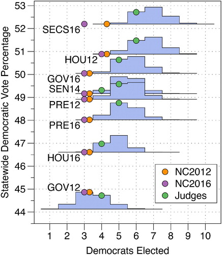
Keeping the vote counts fixed and changing district boundaries does not account for possible effects of incumbency. To reflect a realistic range of incumbency effects, we repeat the above analysis over a range of historic elections that include senatorial, presidential, and gubernatorial races occurring between 2012 and 2016; we also include the 2016 North Carolina Secretary of State race as it has a high statewide Democratic vote fraction. The statewide races have a further advantage over the congressional elections in that that they are not influenced by the district boundaries which we are critiquing. We plot the histograms as a function of the statewide Democratic vote fraction in Figure 2. Each election provides a different tool to probe the properties of the maps under discussion as (i) each election leads to a different statewide fraction, but (ii) each election also contains variations in the spatial patterns of the vote. The NC2012 redistricting plan robustly elects three Democratic candidates in nearly every set of examined historical voting data; the only exceptions are under the 2012 Congressional race and 2016 North Carolina Secretary of State race in which the NC2012 plan would have elected four Democrats. Similarly in the NC2016 redistricting plan robustly elects three Democrats in nearly every set of examined historical voting data; the only exception is under the 2016 North Carolina Secretary of State race in which the NC2016 plan would have elected four Democrats. In contrast, the Judges plan gradually shifts from electing four to six Democrats as the statewide Democratic vote fraction changes from 44% to 52% of the vote; when situated within the ensemble of redistricting plans, the results are nearly always one of the two most expected outcomes; the only exception to this us under the 2014 senate votes under which the Judges plan elects the third most likely set of Democrats. For a table of the histograms see Table S2 in the supplementary materials.

Fig. 2 Distribution of a given number of Democratic wins among the 13 congressional seats using vote counts from a variety of elections. The y-axis shows the statewide democratic vote fraction. Elections shown are the 2012 and 2016 presidential races (PRE12, PRE16), the 2016 North Carolina secretary of state race (SECS16), the 2012 and 2016 gubernatorial races (GOV12, GOV16), the 2014 US senatorial races (SEN14), and the 2012 and 2016 US congressional races (HOU12, HOU16; also shown in Figure 1).

The partisan balance in election outcomes is not the only signature of gerrymandering and gives little detail of the structures that produce the atypical results. Indeed, it is possible for a map to produce a typical fraction of partisan seats, while still having anomalous structures that can impact elections under different voting circumstances (e.g., Herschlag, Ravier, and Mattingly 2017). To further probe the geo-political structure, we order the thirteen congressional districts in any given redistricting plan from the lowest to highest percentage of Democratic votes in each district to construct an ordered thirteen-dimensional vector. For each index, we construct a marginal distribution. We summarize the thirteen distributions in a classical boxplot in Figure 3: To illustrate the construction of this plot, each of the 66,544 sampled plans has a district with the smallest fraction of Democratic votes under the 2012 congressional votes (of its 13 districts); we compute the distribution of smallest Democratic vote fractions to produce the first (leftmost) box in the boxplot. The full extent of the boxplots represent the minimum and maximum observed values and the dashes represent the 1% and 10% outliers. On these boxplots, we overlay the percentage of the Democratic vote for the ordered districts in the NC2012, NC2016, and Judges districting plans. We display the resulting boxplots when considering the 2012 congressional and presidential votes, along with the 2016 congressional and US senate votes.

Fig. 3 We order each district from the smallest to largest Democratic vote fraction. We then examine the vote distribution of the districts smallest, second smallest, etc. vote fractions over the ensemble. The distributions are summarized with boxplots for the congressional voting data from 2012 (left) and 2016 (right), using We compare our statistical results with the three redistricting plans of interest—the NC2012 plan (orange), NC2016 (purple), and Judges plan (green).

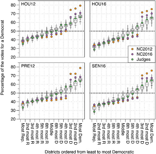
The structure of the boxplot reveals interesting features in the three examined districting plans. The Judge’s districts gradually increase, roughly linearly, from the most Republican district (labeled “Most Rep.”) to the most Democratic (labeled “Most Dem.”); this behavior is identical to the behavior of the marginal distributions. Furthermore, most of the voting percentages from the Judges districts fall inside the boxes on the boxplot which mark the central 50% of the marginal distributions. The NC2012 and NC2016 districting plans have a different structure: Both plans jump in partisan voter percentage between the third and fourth most Democratic districts. In the NC2012 districting plan, the fourth through ninth most Democratic districts have more Republicans than predicted by the ensemble. In the NC2016 districting plan, the fourth through the seventh most Democratic districts have more Republicans than predicted by the ensemble. In both the NC2012 and NC2016 districting plans, Democratic votes are removed from the central districts and added to the three most Democratic districts, all of which have significantly higher Democratic vote fractions than expected—this is strong evidence that Democrats have been concentrated (or packed) in the most Democratic districts, to reduce their influence in the middle districts. This is an illustration of what is commonly referred to as “packing” and “cracking,” in which one party (here the Democrats) has been “packed” or over-represented in some districts, to “crack” or reduce their influence in others.

To quantify this observation, under nearly every historic set of votes, the third most Democratic district of both the NC2012 and NC2016 redistricting plans has a higher Democratic vote fraction than every plan in the ensemble. The only exception to this comes under the 2012 congressional votes in which 59 of the 66,544 ensemble plans have a higher Democratic vote fraction in the third most Democratic district than the corresponding district in the NC2016 plan. Similarly, under nearly every historic election, the fourth most Democratic district of both the NC2012 and NC2016 redistricting plans has a lower Democratic vote fraction than every plan in the ensemble. In this case, the only exception again occurs under the 2012 congressional votes under which 51 of the 66,544 ensemble plans have a lower Democratic vote fraction in the fourth most Democratic district than the corresponding district in the NC2016 plan.

Packing and cracking potentially reduce a party’s political power. When considering the 2012 congressional votes, the boxplot demonstrates that the 4th–6th most Democratic districts are typically above the 50% line, meaning that we expect these districts to elect a Democratic representative; when comparing these districts to the NC2012 and NC2016 districting plans, we see that the 4th–6th most Democratic districts fall below this line, meaning that these districts elected a Republican. When considering the 2016 votes, the NC2012 and NC2016 districting plans lead to a similar change in the delegation’s partisan composition when compared to the ensemble.

In addition to counting the number of elected officials for each party, Figure 3 demonstrates partisan safety—the districts 4th–8th most Democratic districts are all more robustly republican than they would otherwise be. The effect is that elections within these districts may become more robustly Republican. This effect may be seen in both the NC2012 and NC2016 plans for districts labeled six through ten under the 2012 vote counts, and districts labeled eight through ten under the 2016 vote counts.

The Democratic vote fractions of the NC2012 and NC2016 plans show a large jump between the third and fourth most Democratic districts; in comparison, the ensemble and Judges’s plan have ranked districts that increase fairly linearly and gradually in Democratic vote fractions. Under a standard uniform partisan swing hypothesis, a statewide shift in the votes results in the boxplots shifting globally up or down in the direction of the swing (e.g., King and Gelman 1991). Hence, under this assumption, the jump in partisan vote fraction in the NC2012 and NC2016 plans results in a firewall that prevents a change in the partisan seat share over larges changes in voting patterns (including statewide partisan vote shares). This effect is absent from the typical ensemble plans as well as the Judges’s plan and is demonstrated clearly in Figure 2.

The atypical patterns emerging from the NC2012 and NC2016 plans can be viewed as a signature of gerrymandering. This structure further reveals the districts which have had votes from one party removed and dispersed to other districts. The cracking and packing dilutes the Democratic party’s political power. In the next section, we further quantify this signature by contextualizing the plans of interest within the ensemble of redistricting plans when analyzed with summary metrics.

3.1 Summary Metrics

Although we prefer the rich detail provided by the structural portraits shown in Figures 2 and 3, there is a long history of employing summary metrics that seek to encapsulate the above structures with a single number: Such metrics include electoral responsiveness, efficiency gap, the Density-Variation/Compactness, mean-median difference, declination, and more (see, e.g., Gelman and King 1994; Belin, Fischer, and Zigler 2011; Stephanopoulos and McGhee 2015; Wang 2016; Cho and Liu 2016; Warrington 2017). Typically these metrics are contextualized with historical data across past elections, districting plans, and states. However, it is unclear how meaningful the measures are, as they fail to consider the geo-political makeup of a region (see, e.g., Chen and Rodden 2013; Cho 2017). For example, the geo-political makeup of a state may cause it to have a natural partisan bias (Chen and Rodden 2013); in addition to the work in Chen and Rodden (2013), this is also evident in the North Carolina congressional districts as shown in Figure 2, in which the Democrats receive over 50% of the statewide votes in the 2012 Governor’s race, yet will most often only win 5 or 6 of the 13 available seats. For an additional example, see Herschlag, Ravier, and Mattingly (2017), in which it is shown that it is possible for Republicans to win a majority of the state house seats with between 46% and 48% of the vote under non-partisan redistricting plans. Hence, zero partisan-bias might not be a realistic or even desirable goal: The natural structure of the state may not lead to zero partisan bias; forcing zero bias could cause strange artifacts and may necessitate the drawing of strange districts. This is particularly at odds with how such measures are often discussed in the popular press.

Based on these observations, we propose two novel metrics that contextualize a redistricting plan within the underlying space of possible plans. First, we consider the baseline provided by the ordered marginal medians, as shown in Figure 3. For each districting plan, we quantify departures from these medians by considering the standard Euclidean norm between the 13 ordered marginal medians and the observed vote fractions of the ordered districts. To clarify, we let ${\overrightarrow{m}}^{\mathcal{V}}=(m_1,m_2,\dots ,m_{13})$ be the ordered marginal medians of the Democratic vote fractions within the ensemble under the vote counts of election $\mathcal{V}$; we let ${\overrightarrow{\xi }}_i^{\mathcal{V}}=(v_1,v_2,\dots ,v_{13})$ be the ordered vote Democratic fractions of plan ξ_i under the votes given by election $\mathcal{V}$. We define the ranked-marginal deviation for a given districting plan, under a set of specified votes, as(1) $$\left|\right|{\overrightarrow{m}}^{\mathcal{V}}-{\overrightarrow{\xi }}_i^{\mathcal{V}}|{|}_2=\sqrt{\sum _{j=1}^{13}{(m_j-v_j)}^2}.$$(1)

This metric examines deviations in the ordered marginal vote fraction structure. An example and more details on this index are presented in Section S2.2 of the supplementary materials.

Next, we generate a second metric based on the deviation from the expected number of elected Republicans and Democrats. When computing this deviation, we consider a continuous version of the number of elected Democrats in which the integer part of the variable describes the number of elected Democrats and the fractional part represents the relative security between the most competitive Democratic seat and the most competitive Republican seat: To arrive at the relative security we take the linear interpolant between the two seats and intersect it with the 50% vote fraction(2) $$\frac{v_{i+1}-50}{v_i-v_{i+1}},$$(2) where v_i is the ith entry of the ordered Democratic vote fractions from ${\overrightarrow{\xi }}_i^{\mathcal{V}}$ that represents the largest value less than 50%. A value of fewer than 0.5 means that flipping the Democratic seat requires fewer people to change their vote than in the competitive Republican district, and vice versa. We calculate the continuous number of elected Democrats for each districting plan in the ensemble and use the mean of this distribution as a baseline; we define the smoothed seat-count deviation as the distance between the observed number of (continuous) Democrats elected by a given districting plan and the mean of the distribution. An example and more details on this index are presented in Section S2.3 in the supplementary materials.

All of the above-mentioned summary statistics are based on the ordered district vote percentages shown as the dots in Figure 3, however, the two novel statistics also used marginal distributional data shown as the boxplots in Figure 3.

In the present work, we consider two of the established statistics—partisan bias and the efficiency gap. Partisan bias measures the “the extent to which a majority party would fare better than the minority party, should their respective shares of the vote reverse (King 2006)” (see also Gelman and King 1994, and Section S2 of the supplementary materials); the efficiency gap measures the difference between each party’s “wasted votes,” where a vote is wasted if it either does not contribute to a victory or if it was in excess of what was needed for a victory (see Stephanopoulos and McGhee 2015, and Section S2 of the supplementary materials). We also consider the two new proposed statistics. We omit an exhaustive examination of historic metrics as this is not the goal of the present work, however, we remark that our ensemble is publicly available and open for others to examine any measure of interest (see Section S8 in the supplementary materials). Each of the four summary statistics is computed for each redistricting plan in our ensemble and for each districting plan of interest (NC2012, NC2016, and Judges).

We contextualize the partisan bias and the efficiency gap, using the 2012 and 2016 congressional voting data, with histograms in Figure 4. In both statistics and under both vote counts, the NC2012 is an extreme outlier; it shows extreme bias toward the Republican party and wastes an atypical number of Democratic votes. The NC2016 map is not an extreme outlier under either set of vote counts with respect to partisan bias, but is an extreme outlier with respect to the efficiency gap; under both metrics, however, it favors the Republican party. Under the 2012 voting data, only 0.35% of the generated redistricting plans are as, or more, biased than the NC2012 districting plan; 5.4% of the redistricting plans are as, or more, biased than the NC2016. For the 2016 voting data, only 0.24% of the generated redistricting plans are as, or more, biased than the NC2012 districting plan; 6.28% of the plans are as, or more, biased than the NC2016 plan. Under the 2012 and 2016 voting data, the NC2012 districting plan has a higher efficiency gap than all but 0.003% and 0.01% of the generated redistricting plans, respectively. The efficiency gap for the NC2016 map is lower than 0.26% of the redistricting plans in the ensemble for the 2012 voting data, and 0.73% of the redistricting plans in the ensemble for the 2016 voting data.

Fig. 4 Partisan bias (top) and the efficiency gap (bottom) for the three districts of interest and the ensemble of plans. The data are based on the voting data from 2012 (left) and 2016 (right) congressional races.

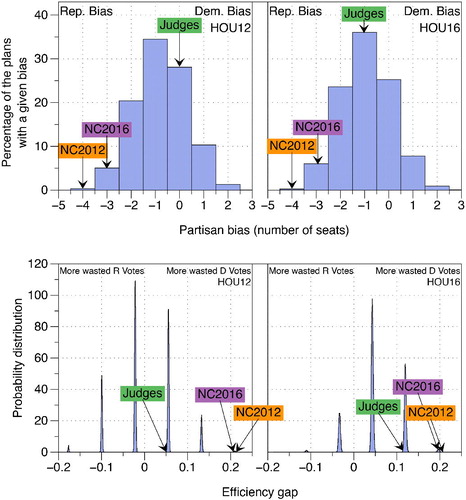
In stark contrast, the Judges districting plan has no partisan bias under the 2012 votes and is only slightly biased under the 2016 votes. Under the 2016 votes, however, the bias in the Judges plan takes on the most likely value of the ensemble. The most likely value in the ensemble favors the Republicans by one seat (i.e., if the Republicans have 55% of the vote, they win one more seat than if Democrats have 55% of the vote). This asymmetry demonstrates the inherent geography of the votes provides a natural advantage to the Republican party in terms of partisan bias. In terms of the efficiency gap, the Judges districting plan wastes fewer Democratic votes than 42.3% of the redistricting plans in the ensemble and 31.0% of redistricting plans under the 2012 and 2016 votes, respectively.

We also contextualize the ranked-marginal deviation (deviation of from median of ordered district votes) and smoothed seat-count deviation (deviation from the expected number of elected representatives) of the three plans of interest within the distribution of the ensemble of plans (see Figure 5). None of the generated redistricting plans constructed have a partisan bias ranked-marginal deviation bigger than NC2012 and NC2016 plans, regardless of the voting data used. Similarly, none of the redistricting plans have a smoothed seat-count deviation greater than NC2012 plan when the 2012 votes are used and only 0.93% of the redistricting plans have a greater smoothed seat-count deviation when the 2016 votes are used. Only 0.003% of the redistricting plans and 0.70% of redistricting plans have a smoothed seat-count deviation greater than NC2016 under the 2012 and 2016 votes, respectively.

Fig. 5 Ranked-marginal deviation (top) and smoothed seat-count deviation (bottom) for the three districts of interest, and the ensemble of plans. Figures are based on the voting data from 2012 (left) and 2016 (right).

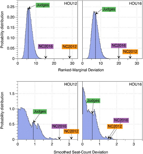
Again, in stark contrast, the Judges districting plan has a lower ranked-marginal deviation than 37.68% redistricting plans and 55.04% redistricting plans under the 2012 and 2016 votes, respectively. Similarly, the Judges districting plan has a lower smoothed seat-count deviation than 26.39% and 33.88% of the redistricting plans in the ensemble under the 2012 and 2016 votes, respectively.

All four metrics over both election years indicate that the Judges plan is very typical. The Judges plan shows low partisan bias, has a reasonable efficiency gap, has a comparatively low level of gerrymandering, and is reasonably representative. In contrast, the NC2012 and NC2016 plans have a strong partisan bias toward the republicans, have a large efficiency gap, are unrepresentative, and are highly gerrymandered.

While some might like the persuasive simplicity of a single number and arguments which state that the chosen metric is an outlier, we prefer the more descriptive images of Figures 2 and 3 along with the outlier status of the packing and cracking they identify. We find these more explanatory and prefer leading with understanding rather than generic, one-size-fits-all statistical tests. We find statistical characterizations most compelling when directly supporting the narrative already suggested by the visualizations.

3.2 Comparing to Locally Similar Redistricting Plans

If relatively small changes in a redistricting plan dramatically change the partisan vote balance in each district then it raises questions how representative the results generated by the redistricting plan are, and suggests the redistricting plan was selected or engineered.²

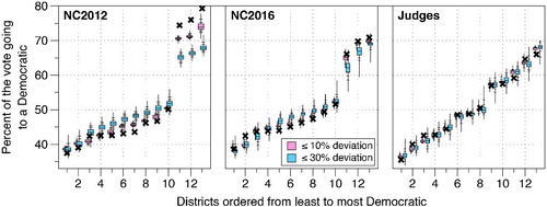
We explore the degree to which the three most Democratic districts of NC2012 and NC2016 are locally typical by examining local ensembles that preserve the core districts on each of the three plans. When generating these new ensembles, we require that each district in the ensemble directly corresponds to a district within a plan of interest and that its population deviates no more than a certain percentage away from the original district. We generate six new ensembles, two for each plan, that deviate by no more than 10% and 30% of the population on each district. Details on the generative procedure and on the ensembles are presented in Section S6 of the supplementary materials.

We display our results in Figure 6 under the 2012 congressional votes. We find that in the NC2012 and NC2016 districts, the top three democratic districts of the two local ensembles precipitously lose Democratic voters and this effect continues as the districts are allowed to deviate more. In contrast, in the Judges plan, there is no appreciable trend of how the structure of the local districts deviate, save some spreading of the marginal distributions. In other words, small changes to district boundaries make the NC2012 and NC2016 redistricting plans less partisan but do not change the characteristics of the Judges redistricting plan. This suggests that NC2012 and NC2016 plans, in contrast to the Judge’s plan, were precisely engineered to achieve a partisan goal.

Fig. 6 We display the ranked marginal distributions based on random samples drawn from nearby the three redistricting plans of interest: NC2012 (left), NC2016 (center), and Judges (right). Black X’s mark the plans ranked district margins, whereas light purple and turquoise boxplots mark the 10% and 30% deviations, respectively. All plots use the 2012 congressional votes.

4 Discussion

We have found that in most electoral settings, the NC2012 and NC2016 districting plans give the Republicans an advantage relative to an ensemble of neutrally drawn maps. This advantage manifests as the number of elected officials and as abnormally safe margins of victory. The abnormally safe margins are related to an abnormal jump in the ranked ordered district structure, and reveal a signature of what would be expected when there has been intentional partisan manipulation of districts. The abnormal jump makes the partisan seat make up insensitive to plausible swings in public voting patterns as demonstrated in Figure 2. Across a number of historic voting patterns, we have found that on one side of the jump, there are districts packed with Democratic votes. These Democrats have been cracked from the districts on the other side of the jump, where we have observed districts with fewer Democratic voters than expected.

There is a long history of quantifying gerrymandering with metrics that yield a single number. We do not think this is the most effective method of conveying the structure and consequence of gerrymandering. We prefer discussing structural differences revealed by the rank-ordered marginal distributions. The single number metrics are particularly useful when supporting and quantifying qualitative observations from the rank-ordered marginal distributions.

We have examined the single number metrics of partisan bias, the efficiency gap, as well as two new measures that we have deemed the ranked-marginal deviation and smoothed seat-count deviation. We have identified abnormal behavior in the enacted maps based on these metrics by comparing them with the distribution of the metric evaluated across the ensemble. We continue to stress that such outlying behavior accounts for the geo-political landscape of the state. Under all four of these measures, we again find that the NC2012 and NC2016 redistricting plans are often extreme outliers, further suggesting that (i) these districts are heavily gerrymandered and (ii) do not represent the geo-political landscape expressed in a number of elections occurring between 2012 and 2016. Further analysis reveals the NC2012 and NC2016 plans are locally engineered for partisan benefit. All of these results are consistent with the findings of Liu, Cho, and Wang (2016).

In contrast, the districting plan produced by a bipartisan redistricting commission of retired judges from the Beyond Gerrymandering project produced results that are comfortably within the range of typical variations across plans generated without reference to partisan criteria. The Judges plan is not gerrymandered, was typically representative of the people’s will, and displayed consistent statistics with nearby redistricting plans.

We can extend the ideas of this report to analyze state legislatures, congressional districts in other states, and other types of local districting plans. We note that each state may have different requirements when drawing district boundaries, so care must be taken when considering the criteria to be included in the generative procedure. We hope that the analysis in this report is utilized across different states and levels of government to test the viability of districting plans.

As stated in the introduction, the qualitative results and subsequent conclusions of this article are consistent with those in earlier iterations of this analysis reported in Bangia et al. (2017), based on an ensemble generated in a slightly different manner. We have taken the opportunity of this report to improve upon the convergence validations used in generating our ensemble (see Section S4 in the supplementary materials). We have also expanded our analysis to include more statewide elections both because we have grown to prefer statewide elections and generally because each election provides a different tool to probe the properties of the maps under discussion. Each election has a different statewide vote fraction but also different spatial patterns of votes. We have also taken the opportunity to correct a miscalculation of proposal transition probabilities in Bangia et al. (2017). In practice, this had little effect on the Markov chain as witnessed by the close agreement of the results of this note and Bangia et al. (2017).

As a practical tool, the methods presented in this work, as well as similar tools have already been used in several court cases to identify gerrymandering (LWV 2018; Com 2019a, 2019b). Indeed, these methods have typically, thus far, been used as a tool to audit a given redistricting plan. We see no reason why this tool cannot be used to audit plans once they are proposed by legislatures or independent commissions. In this setting map drawing bodies that claim to have not used partisanship when drawing maps may be checked with such statistical methods. Alternatively, one could use these methods to find acceptable ranges of partisanship while in the process of drawing a map, however, we believe that this is a far more dangerous application as map drawing bodies could engineer maps that favor their parties as much as possible within the bounds prescribed by an ensemble.

We wish to emphasize that the generation of the ensemble is separate from its analysis. For example, one could critique our ensemble for generating districts that are too compact, or not compact enough. In either case, we can change the underlying target distribution and sampling procedure to focus on a new regime of the space of redistricting plans and investigate whether or results change. In the case of the above example, we have found that our results are robust to changes in the allowable compactness (see Section S5.3 in the supplementary materials). As another example, the map-drawing body may come out and claim that keeping certain communities intact was a crucial part of the redistricting process; again, the score function can be altered to preserve such communities. In short, the ensemble is able to probe any number of proclaimed redistricting factors to investigate their effect on the expected partisan election outcomes.

We also wish to emphasize that using each historic vote count provides a unique probe on a plausible set of vote counts under which we can compare the ensemble of maps to a given map. The historic votes are not meant to be predictive of future elections, but rather to be used as a collection of lenses upon which to test whether a given plan exhibits extreme statistical properties with respect to the ensemble.

Finally, the current methodology employs simulated annealing paired with Markov chain Monte Carlo sampling techniques. We have demonstrated that our methodology converges to a robust result, however, we have not provided guarantees that the target probability distribution agrees with the sampled distribution beyond valuing the same regions of high probability. Sampling directly using MCMC without simulated annealing in the current context will only become possible under more sophisticated sampling techniques with a fixed measure, and these techniques are the subject of our future research. Directly sampling using the MCMC described here has already been used successfully to analyze the North Carolina State Legislative districts and presented to the court in Common Cause v. Lewis.

Supplementary Materials

The supplemental material contains (i) details on how we sample from the space of redistricting plans, (ii) further details on the indices used in Section 3.1, and details on the utilized data, including the HB92 criteria, voting data, the enacted NC2012 and NC2016 districting plans, the Judges districting plan, (iii) numerical values over the histograms presented in Figures 1 and 2, (iv) convergence analyses on our MCMC algorithm, (v) sensitivity and error analyses for how our results are insensitive to change due to splitting VTDs to achieve zero population, changing the target measure, changing the sampling procedure, and redefining the space of allowable maps, and (vi) a discussion of the properties of the ensemble of maps including county splitting and compactness properties.

Acknowledgments

A preliminary version of the results presented in this article were first reported to the arXiv repository (Bangia et al. 2017). Bridget Dou and Sophie Guo were integral members of the Quantifying Gerrymandering Team and have significantly influenced this work. Mark Thomas, and the Duke Library GIS staff helped with data extraction. Robert Calderbank, Galen Reeves, Henry Pfister, Scott de Marchi, and Sayan Mukherjee have provided help throughout this project. John O’Hale procured the 2016 election Data. Tom Ross, Fritz Mayer, Land Douglas Elliott, and B.J.Rudell invited us observe the Beyond Gerrymandering Project and this work relies on what we learned there.

Funding

The Duke Math Department, the Information Initiative at Duke (iID), the PRUV, and Data + undergraduate research programs provided financial and material support.

References

- Bangia, S., Graves, C. V., Herschlag, G., Kang, H. S., Luo, J., Mattingly, J. C., and Ravier, R. (2017), “Redistricting: Drawing the Line,” arXiv no. 1704.03360.
- Belin, T. R., Fischer, H. J., and Zigler, C. M. (2011), “Using a Density-Variation/Compactness Measure to Evaluate Redistricting Plans for Partisan Bias and Electoral Responsiveness,” Statistics, Politics, and Policy, 2, 1–27. DOI: 10.2202/2151-7509.1020.
- Chen, J., and Rodden, J. (2013), “Unintentional Gerrymandering: Political Geography and Electoral Bias in Legislatures,” Quarterly Journal of Political Science, 8, 239–269. DOI: 10.1561/100.00012033.
- Chikina, M., Frieze, A., and Pegden, W. (2017), “Assessing Significance in a Markov Chain Without Mixing,” Proceedings of the National Academy of Sciences of the United States of America, 114, 2860–2864. DOI: 10.1073/pnas.1617540114.
- Cho, W. K. T. (2017), “Measuring Partisan Fairness: How Well Does the Efficiency Gap Guard Against Sophisticated As Well As Simple-Minded Modes of Partisan Discrimination?,” University of Pennsylvania Law Review Online, 166.
- Cho, W. K. T., and Liu, Y. Y. (2016), “Toward a Talismanic Redistricting Tool: A Computational Method for Identifying Extreme Redistricting Plans,” Election Law Journal, 15, 351–366. DOI: 10.1089/elj.2016.0384.
- “Common Cause v. Rucho no. 18-422, 588 U.S. ___” (2019a).
- “Corman v. Torres Case 1:18-CV-00443 PA___” (2018).
- Gelman, A., and King, G. (1994), “Enhancing Democracy Through Legislative Redistricting,” American Political Science Review, 88, 541–559. DOI: 10.2307/2944794.
- Herschlag, G., and Mattingly, J. (2018), “Quantifying Gerrymandering Blog,” available at https://sites.duke.edu/quantifyinggerrymandering/.
- Herschlag, G., Ravier, R., and Mattingly, J. C. (2017), “Evaluating Partisan Gerrymandering in Wisconsin,” arXiv no. 1709.01596.
- King, G. (2006), “Amici Curiae League of United Latin Am. Citizens v. Perry,” 548 U.S. 399.
- King, G., and Gelman, A. (1991), “Systematic Consequences of Incumbency Advantage in the U.S. House Elections,” American Journal of Political Science, 35, 110–138. DOI: 10.2307/2111440.
- Lander, E. S. (2017), “Brief for Amicus Curiae Eric S,” Lander in Support of Appellees.
- Lebovici, L., Eure, S., Ramesh, R., Herschlag, G., and Mattingly, J. (2018), “Gerrymandering and the Extent of Democracy in America,” available at https://bigdata.duke.edu/projects/gerrymandering-and-extent-democracy-america.
- “Lewis v. Common Cause Superior Court Division 18 CVS 014001 Wake County NC___” (2019b).
- Liu, Y. Y., Cho, W. K. T., and Wang, S. (2016), “Pear: A Massively Parallel Evolutionary Computation Approach for Political Redistricting Optimization and Analysis,” Swarm and Evolutionary Computation, 30, 78–92.
- Mattingly, J. C., and Vaughn, C. (2014), “Redistricting and the Will of the People,” arXiv no. 1410.8796.
- Stephanopoulos, N. O., and McGhee, E. M. (2015), “Partisan Gerrymandering and the Efficiency Gap,” University of Chicago Law Review, 82, 831.
- Tom Ross and POLIS Center at Duke (2016), “Beyond Gerrymandering Project,” available at https://sites.duke.edu/polis/projects/beyond-gerrymandering/.
- Wang, S. S.-H. (2016), “Three Tests for Practical Evaluation of Partisan Gerrymandering,” Stanford Law Review, 68, 1263.
- Warrington, G. S. (2017), “Quantifying Gerrymandering Using the Vote Distribution,” arXiv no. 1705.09393.