Separating Effect From Significance in Markov Chain Tests

Abstract

We give qualitative and quantitative improvements to theorems which enable significance testing in Markov chains, with a particular eye toward the goal of enabling strong, interpretable, and statistically rigorous claims of political gerrymandering. Our results can be used to demonstrate at a desired significance level that a given Markov chain state (e.g., a districting) is extremely unusual (rather than just atypical) with respect to the fragility of its characteristics in the chain. We also provide theorems specialized to leverage quantitative improvements when there is a product structure in the underlying probability space, as can occur due to geographical constraints on districtings.

Keywords:

• Gerrymandering
• Markov chain
• Outlier

This note discusses improvements on a number of theorems for significance testing in Markov chains. The improvements to the theorem statements are both qualitative and quantitative to enable strong, easily interpretable statistical claims, and include extensions to settings where more structural assumptions lead to dramatic improvements in the bounds. This class of theorems is of particular interest because they do not assume that the chain has converged to equilibrium, which is of practical importance since the mixing time of Markov chains used in applications is frequently unknown.

The development of this class of algorithms and these particular extensions have been directly motivated by a question of significant contemporary interest; detecting and quantifying gerrymandering. The definiteness and correctness provided by these theorems affords decision makers (e.g., in a legal setting) with an uncommonly rigorous approach to understanding whether a political districting is carefully crafted for partisan advantage. These methods (and theorems) have been used successfully by one of the authors in Gerrymandering court cases in Pennsylvania and North Carolina.

The first technical part of this article gives new results along these lines, extending the work in Chikina, Frieze, and Pegden (2017) to allow separation of effect size from the quantification of statistical significance. The second part, in Section 8, develops versions of some of these results in a special setting with a particular structure on the probability space motivated by recent legal proceedings. In particular, in balancing the federal one-person-one-vote mandate with the “keep counties whole” prevision of the North Carolina Constitution, the North Carolina courts ruled in Stephenson v. Bartlett that a particular algorithm should be used to “cluster” the counties into independent county groups which are districted separately. This gives a product structure to the underlying probability space which can be exploited in theorems designed to take advantage of it.

In Section 1, we consider the technical background and past results necessary to frame the new results of this article; in Section 2, we discuss the practical challenges which motivate the new theoretical framework we develop in this article. The new results are stated and discussed in Section 3. Later sections prove the new theorems.

1 Background and Previous Results

Consider a reversible Markov chain $\mathcal{M}$ whose state-space Σ is endowed with some labeling $\omega :\Sigma \to \mathbb{R}$, and for which π is a stationary distribution. $\mathcal{M}$, π, ω, and a fixed integer k determine a vector$$p_0^k,p_1^k,\dots ,p_k^k,$$where for each i, $p_i^k$ is the probability that for a k-step π-stationary trajectory $X_0,\dots ,X_k$, the minimum ω value occurs at X_i . In other words, $p_i^k$ is the probability that if we choose X ₀ randomly from the stationary distribution π and take k steps in $\mathcal{M}$ to obtain the trajectory $X_0,X_1,\dots ,X_k$, that we observe that $\omega (X_i)$ is the minimum among $\omega (X_0),\dots ,\omega (X_k)$. Note that if we adopted the convention that we break ties among the values $\omega (X_0),\dots ,\omega (X_k)$ randomly, we would have that $p_0^k+\cdots +p_k^k=1$, for any $\mathcal{M},\pi ,$ and k.

In the context of districting, $\mathcal{M}$ is generally a random walk on the space of possible districtings of a state; for example, from one districting, we can randomly choose a voting precinct on the boundary of two districts, and switch its district membership if doing so does not violate constraints on contiguity, population deviation, etc. (see Figure 1 for an example of such a move). This transition rule defines a reversible Markov chain on the state space consisting of all valid districtings of the state. The label function ω could be, for example, the partisanship of any given districting—which could be defined, for example, from simulated election results using historical voting data. In this context, $p_0^k$ is the probability that if began from a random districting of a state, and carried out a sequence of k random transitions, that the initial districting in the sequence would be the most partisan districting observed in the sequence.

Fig. 1 An example of a Markov chain transition for the legislative districting of Wisconsin.

At first glance, it might be natural to assume that we must have something like $p_i^k\approx \frac{1}{k+1}$ for all $0\le i\le k$. This would mean, for example, that if we generated a sequence of 10,000 districtings, and the initial districting was the most partisan, that it would be valid to conclude that the initial districting was not randomly chosen from the stationary distribution, at a p-value of p = 0.0001. But this is actually quite far from the truth; Chikina, Frieze, and Pegden (2017) showed that for some $\mathcal{M},\pi ,k$, we can have $p_0^k$ as large as essentially $\frac{1}{\sqrt{2\pi k}}$.

As shown in Chikina, Frieze, and Pegden (2017), this is essentially the worst possible behavior for $p_0^k$. In particular, we can generalize the vector $\left\{p_i^k\right\}$ defined above as possible: let us define, given $\mathcal{M},\pi$, k, and $0\le \epsilon \le 1$, the vector$$p_{0,\epsilon }^k,p_{1,\epsilon }^k,\dots ,p_{k,\epsilon }^k,$$where each $p_{i,\epsilon }^k$ is the probability that $\omega (X_i)$ is among the smallest ε fraction of values in the list $\omega (X_0),\dots ,\omega (X_k)$. Then in Chikina, Frieze, and Pegden (2017) we proved:

Theorem 1.1.

Given a reversible Markov chain $\mathcal{M}$ with stationary distribution π, an $\epsilon >0,k\ge 0$ , and with $p_{i,\epsilon }^k$ defined as above, we have that $$p_{0,\epsilon }^k\le \sqrt{2\epsilon }.$$

In particular, in the case of the first districting which is most partisan on a sequence of 10,000, this supports a p-value of $p=\sqrt{2}/100\approx 0.014$. Note that the example from Chikina, Frieze, and Pegden (2017) realizing $p_0^k\approx \frac{1}{\sqrt{2\pi k}}$ shows that this theorem is best possible, up to constant factors.

As indicated by the example of making a sequence of random changes to a districting, one important application of Theorem 1.1 is that it characterizes the statistical significance associated to the result of the following natural test for gerrymandering of political districtings:

Local outlier test

1. Beginning from the districting being evaluated,

2. Make a sequence of random changes to the districting, while preserving some set of constraints imposed on the districtings.

3. Evaluate the partisan properties of each districting encountered (e.g., by simulating elections using past voting data).

4. Call the original districting “carefully crafted” or “gerrymandered” if the overwhelming majority of districtings produced by making small random changes are less partisan than the original districting.

Naturally, the test described above can be implemented so that it precisely satisfies the hypotheses of Theorem 1.1. For this purpose, a (very large) set of comparison districtings are defined, to which the districting being evaluated belongs. For example, the comparison districtings may be the districtings built out of Census blocks (or some other unit) which are contiguous, equal in population up to some specified deviation, or include other constraints. A Markov chain $\mathcal{M}$ is defined on this set of districtings, where transitions in the chain correspond to changes in districtings. (E.g., a transition may correspond to randomly changing the district assignment of a randomly chosen Census block which currently borders more than one district, subject to the constraints imposed on the comparison set.) The “random changes” from Step 2 will then be precisely governed by the transition probabilities of the Markov chain $\mathcal{M}$. By designing $\mathcal{M}$ so that the uniform distribution π on the set of comparison districtings Σ is a stationary distribution for $\mathcal{M}$, Theorem 1.1 gives an upper bound on the false-positive rate (in other words, global statistical significance) for the “gerrymandered” declaration when it is made in Step 4.

Remark 1.1. N

ote that while a local outlier test can be used to give a statistical significant finding of gerrymandering, it cannot be used alone to demonstrate rigorously that a districting is not gerrymandered. In particular, when a districting does not seem gerrymandered to a local outlier test, it is quite possible that the chain is simply not mixing well enough to explore the space of alternatives. The theorems discussed in this article give one-way guarantees: for example, observing outlier status confers a statistically significant finding of gerrymandering, but failing to observe it is inconclusive, absent other evidence.

Apart from its application to gerrymandering, Theorem 1.1 has a simple informal interpretation for the general behavior of reversible Markov chains, namely: typical (i.e., stationary) states are unlikely to change in a consistent way under a sequence of chain transitions, with a best-possible quantification of this fact (up to constant factors).

Also, in the general setting of a reversible Markov chain, the theorem leads to a simple quantitative procedure for asserting rigorously that σ ₀ is atypical with respect to π without knowing the mixing time of $\mathcal{M}$: simply observe a random trajectory ${\sigma }_0=X_0,X_1,X_2,\dots ,X_k$ from σ ₀ for any fixed k. If $\omega ({\sigma }_0)$ is an ε-outlier among $\omega (X_0),\dots ,\omega (X_k)$, then this is statistically significant at $\sqrt{2\epsilon }$ against the null hypothesis that ${\sigma }_0\sim \pi$.

This quantitative test is potentially useful because $\sqrt{2\epsilon }$ converges quickly enough to 0 as $\epsilon \to 0$; in particular, it is possible to obtain good statistical significance from observations which can be made with reasonable computational resources. Of course, faster convergence to 0 would be even better, but, as already noted, $p\approx \sqrt{\epsilon }$ is roughly a best possible upper bound.

On the other hand, it is possible to achieve better dependence on ε by changing the parameters of the test. For example, we will prove the following theorem as a stepping-stone to the main results of the present manuscript:

Theorem 1.2.

Consider two independent trajectories $Y_0,\dots ,Y_k$ and $Z_0,\dots ,Z_k$ in the reversible Markov chain $\mathcal{M}$ (whose states have real-valued labels) from a common starting point $Y_0=Z_0={\sigma }_0$. If we choose σ ₀ from a stationary distribution π of $\mathcal{M}$, then for any k we have that$$\begin{array}{c}\text{Pr}(\omega ({\sigma }_0)\text{is}\mathrm{ }\text{an}\mathrm{ }\epsilon -\text{outlier}\mathrm{ }\text{among}\mathrm{ }\omega ({\sigma }_0),\omega (Y_1),\dots ,\\ \mathrm{\hspace{1em}}\mathrm{\hspace{1em}}\omega (Y_k),\omega (Z_1),\dots ,\omega (Z_k))<2\epsilon .\end{array}$$

Note that due to the reversibility of the chain, Theorem 1.2 is equivalent to the statement that the probabilities $p_{i,\epsilon }^k$ always satisfy(1) $$p_{k,\epsilon }^{2k}<2\epsilon .$$(1)

Remark 1.2. A

s in the case of Theorem 1.1, it seems like an interesting question to investigate the tightness of the constant 2; we will see in Section 8 that there are settings where the impact of this constant is inflated to have outsize-importance. We point out here that at least for the case of k = 1, $\epsilon =1/3,{\rho }_{1,\frac{1}{3}}^2$ can be at least as large as $\frac{1}{2}$, showing that the constant 2 in (1) cannot be replaced by a constant less than $\frac{3}{2}$, in general. To see this, consider, for example, a bipartite complete graph $K_{n,n}$, where the labels of the vertices of one side are $1,\dots ,n$ and the other are $n+1,\dots ,2n$. For the Markov chain given by the random walk on this undirected graph, we have that ${\rho }_{1,\frac{1}{3}}^2=\frac{1}{2}$. Note that for this example, it is still the case that ${\rho }_{k,\epsilon }^{2k}\to \epsilon$ as $k\to \infty$, leaving open the possibility that the 2 in (1) can be replaced with an expression asymptotically equivalent to 1.

The informal interpretation of Theorem 1.2 is thus: typical (i.e., stationary) states are unlikely to change in a consistent way under two sequences of chain transitions.

Unknown to the authors at the time of the publication of Chikina, Frieze, and Pegden (2017), Besag and Clifford (1989) described a test related to that based on Theorem 1.2, which has essentially a one-line proof, which we discuss in Section 5:

Theorem 1.3

(Besag and Clifford serial test). Fix any number k and suppose that σ ₀ is chosen from a stationary distribution π, and that ξ is chosen uniformly in $\{0,\dots ,k\}$. Consider two independent trajectories $Y_0,Y_1,\dots$ and $Z_0,Z_1,\dots$ in the reversible Markov chain $\mathcal{M}$ (whose states have real-valued labels) from $Y_0=Z_0={\sigma }_0$. If we choose σ ₀ from a stationary distribution π of $\mathcal{M}$, then for any k we have that$$\begin{array}{c}\text{Pr}(\omega ({\sigma }_0)\text{is}\mathrm{ }\text{an}\mathrm{ }\epsilon -\text{outlier}\mathrm{ }\text{among}\mathrm{ }\omega ({\sigma }_0),\omega (Y_1),\dots ,\\ \mathrm{\hspace{1em}}\mathrm{\hspace{1em}}\omega (Y_{\xi }),\omega (Z_1),\dots ,\omega (Z_{k-\xi }))\le \epsilon .\end{array}$$

Here, a real number a ₀ is an ε-outlier among $a_0,\dots ,a_k$ if$$\#\left\{i\in \{0,\dots ,k\}|a_i\le a_0\right\}\le \epsilon (k+1).$$

In particular, the striking thing about Theorem 1.3 is that it achieves a best-possible dependence on the parameter ε. (Notice that ε would be the correct value of the probability if, for example, the Markov chain is simply a collection of independent random samples.) The sacrifice is in Theorem 1.3’s slightly more complicated intuitive interpretation, which would be: typical (i.e., stationary) states are unlikely to change in a consistent way under two sequences of chain transitions of random complementary lengths. Note that the pattern in these theorems is that the simplicity of the intuitive interpretation of the theorem is sacrificed for the quantitative bounds offered; one goal of the present article is prove theorems which avoid this trade off.

2 The Need for New Statistical Approaches

In late 2018, the nonprofit Common Cause filed a lawsuit in North Carolina superior court challenging the state-level districting plans (for the North Carolina state House and Senate districts). The third and fourth authors of this article served as expert witnesses in this case, which ultimately found the challenged districtings to be unconstitutional partisan gerrymanders. In this section, we use some of the findings from the fourth author’s expert report Pegden (2019) in that case as motivation for the need for the new theoretical results we advance in this article.

One interesting feature of districting in North Carolina is the requirement (from the state supreme court case Stephenson v. Bartlett) that districtings of that state must respect particular groupings—county clusters—determined, essentially deterministically, by a prescribed set of rules.

A complete districting of the state of North Carolina is thus composed of completely separate, noninteracting districting problems in each county cluster. One practical question of interest in Common Cause v. Lewis—separate from the question of whether the challenged districtings were partisan gerrymanders—was the question of which specific county clusters were gerrymandered in each (House and Senate) districting.

The basic approach of the analysis used in Pegden (2019) begins with an experiment in which random changes are made to the actual, enacted districting of the state being evaluated. For example, Table 1 (taken from Pegden (2019)) shows the results of 16 such experiments run on the North Carolina House districting:

Table 1 Results of the analysis from Pegden (2019) for the House districting of North Carolina.

Run	Percentage of comparison maps less partisan than enacted plan	Run	Percentage of comparison maps less partisan than enacted plan	Run	Percentage of comparison maps less partisan than enacted plan	Run	Percentage of comparison maps less partisan than enacted plan
1	99.999994%	5	99.9999999964%	9	99.999997%	13	99.99984%
2	99.99999999963%	6	99.9999999988%	10	99.99999999909%	14	99.9999999986%
3	99.99999999981%	7	99.99999945%	11	99.9999999949%	15	99.9999948%
4	99.9999984%	8	99.999998%	12	99.9999982%	16	99.9999999973%

Each number shows, as a percentage, the fraction of districtings encountered in the sequence of random changes which were more Republican-favorable than the enacted plan. The particular choices of partisan metrics and voting data can be found in Pegden (2019). (Figure 2 shows the initial map as well as three examples of maps encountered in the first experiment.)

Fig. 2 First: The challenged State House districting of North Carolina, and three examples of maps encountered by a sequence of random changes.

The percentages recorded in Table 1 show that the enacted House plan is an extreme outlier among the plans generated by making small random changes to the enacted plan. This already gives strong intuitive evidence that the enacted plan is extremely carefully drawn to maximize partisan advantage: as soon as the lines of the map are subjected to small random changes, the overwhelming fraction of encountered maps are less advantageous to Republicans than the enacted plan.

But the next step of the analysis in Pegden (2019) is the application of rigorous theorems to establish statistical significance for the findings in Table 1. This is slightly subtle, since, as we will see when setting up the technical details later, we do not make the heuristic assumption that the randomly generated plans are uniform samples from some set of possible maps; instead, we wish to make rigorous statistical claims with respect to the actual experiment, a Markovian process of making a sequence of random changes to the initial map.

The previous paper (Chikina, Frieze, and Pegden 2017) also took this approach in an analysis of the Congressional districting of Pennsylvania (which later formed the basis of expert testimony in the League of Women Voters v. Pennsylvania case which challenged the Congressional districting there). The theorem from Chikina, Frieze, and Pegden (2017) allows one to establish statistical significance of $p=\sqrt{2\epsilon }$ when one finds that a $1-\epsilon$ fraction of maps are less advantageous to (say) the Republicans than the enacted map. For example, for Run 1 in Table 1, $\epsilon =0.00000006$ and so p = 0.0003 is quite statistically significant, against the null hypothesis of a randomly chosen districting.

But an important question in the Common Cause v. Lewis lawsuit was not simply whether unconstitutional gerrymandering took place in the drawing of the North Carolina plans, but in which county clusters it took place (so that districtings in those clusters could be ordered redrawn). As an example we will consider the county cluster consisting of Forsyth and Yadkin counties; the challenged map and 3 examples of maps encountered by the sequence of random changes are shown in Figure 3, while the table of results for this cluster are shown in Table 2. While Table 2 shows that the overwhelming fraction of maps encountered by making random changes were less favorable to Republicans, ε values of around 0.002 in this case are not small enough that $\sqrt{2\epsilon }$ would be statistically significant. In particular, even if we applied a test like that given by Theorem 1.2 or Theorem 1.3, our level of statistical confidence would be limited by the degree to which the districting in this county cluster is an outlier.

Fig. 3 First: The challenged State House districting within the Forsyth-Yadkin county cluster, and three examples of maps encountered by a sequence of random changes to this districting.

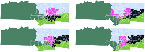
Table 2 Results of the analysis from Pegden (2019) for the House districting of North Carolina in the Forsyth-Yadkin cluster.

Run	Percentage of comparison maps less partisan than enacted plan	Run	Percentage of comparison maps less partisan than enacted plan	Run	Percentage of comparison maps less partisan than enacted plan	Run	Percentage of comparison maps less partisan than enacted plan
1	99.945%	9	99.905%	17	99.87%	25	99.92%
2	99.76%	10	99.925%	18	99.84%	26	99.84%
3	99.87%	11	99.8%	19	99.929%	27	99.81%
4	99.86%	12	99.911%	20	99.73%	28	99.85%
5	99.77%	13	99.8%	21	99.88%	29	99.83%
6	99.89%	14	99.927%	22	99.906%	30	99.77%
7	99.91%	15	99.82%	23	99.8%	31	99.947%
8	99.79%	16	99.88%	24	99.88%	32	99.937%

Instead, we wish to decouple the statistical significance of our finding from the level of outlier status we can report for the districting in this cluster; this is a major goal of the approach we take in this note.

3 New Results

One common feature of the tests based on Theorems 1.1 and 1.3 is the use of randomness. In particular, the probability space at play in these theorems includes both the random choice of σ ₀ assumed by the null hypothesis and the random steps taken by the Markov chain from σ ₀. Thus, the measures of “how (globally) unusual” σ ₀ is with respect to its performance in the local outlier test and “how sure” we are that σ ₀ is unusual in this respect are intertwined in the final p-value. In particular, the effect size and the statistical significance are not explicitly separated.

To further the goal of simplifying the interpretation of the results of these tests, our approach in this note will also show that tests like these can be efficiently used in a way which separates the measure of statistical significance from the question of the magnitude of the effect. For example, our new results would allow one to capture the outlier status of a cluster like Forsyth-Yadkin discussed in the previous section, at a p-value which can be made arbitrarily small, independent of the observed ε values.

To begin, let us recall the probabilities $p_{0,\epsilon }^k,\dots ,p_{k,\epsilon }^k$ defined previously, let us define the ε-failure probability $p_{0,\epsilon }^k({\sigma }_0)$ to be the probability that on a trajectory ${\sigma }_0=X_0,X_1,\dots ,X_k,\omega ({\sigma }_0)$ is among the smallest ε fraction of the list $\omega (X_0),\dots ,\omega (X_k)$. Now we make the following definition:

Definition 3.1.

With respect to k, the state σ ₀ is an $(\epsilon ,\alpha )$-outlier in $\mathcal{M}$ if, among all states in $\mathcal{M},p_{0,\epsilon }^k({\sigma }_0)$ is in the largest α fraction of the values of $p_{0,\epsilon }^k(\sigma )$ over all states $\sigma \in \mathcal{M}$, weighted according to π.

In particular, being an $(\epsilon ,\alpha )$-outlier measures the likelihood of σ ₀ to fail the local outlier test, ranked against all other states $\sigma \sim \pi$ of the chain $\mathcal{M}$. For example, fix $k={10}^9$. If σ ₀ is a $({10}^{-6},{10}^{-5})$-outlier in $\mathcal{M}$ and π is the uniform distribution, this means that among all states $\sigma \in \mathcal{M}$, σ ₀ is more likely than all but a ${10}^{-5}$ fraction of states to have an ω-value in the bottom ${10}^{-6}$ values $\omega (X_0),\omega (X_1),\dots ,\omega (X_{{10}^9})$. Note that the probability space underlying the “more likely” claim here just concerns the choice of the random trajectory $X_1,\dots ,X_{{10}^9}$ from $\mathcal{M}$.

Note that whether σ ₀ is a $(\epsilon ,\alpha )$-outlier is a deterministic question about the properties of ${\sigma }_0,\mathcal{M},$ and ω. Thus, it is a deterministic measure (defined in terms of certain probabilities) of the extent to which σ ₀ is unusual (globally, in all of $\mathcal{M}$) with respect to its local fragility in the chain.

The following theorem enables one to assert statistical significance for the property of being an $(\epsilon ,\alpha )$-outlier. In particular, while tests based on Theorems 1.1 and 1.3 take as their null hypothesis that ${\sigma }_0\sim \pi$, the following theorem takes as its null hypothesis merely that σ ₀ is not an $(\epsilon ,\alpha )$-outlier.

Theorem 3.1.

Consider m independent trajectories$$\begin{array}{c}{\mathcal{T}}^1= (X_0^1,X_1^1,\dots ,X_k^1),\\ ⋮\\ {\mathcal{T}}^m= (X_0^m,X_1^m,\dots ,X_k^m)\end{array}$$of length k in the reversible Markov chain $\mathcal{M}$ (whose states have real-valued labels) from a common starting point $X_0^1=\dots =X_0^m={\sigma }_0$. Define the random variable ρ to be the number of trajectories ${\mathcal{T}}^i$ on which σ ₀ is an ε-outlier.

If σ ₀ is not an $(\epsilon ,\alpha )$-outlier, then(2) $$\text{Pr}\left(\rho \ge m\sqrt{\frac{2\epsilon }{\alpha }}+r\right)\le e^{-\min (r^2\sqrt{\alpha /2\epsilon }/3m,r/3)}.$$(2)

In particular, apart from separating measures of statistical significance from the quantification of a local outlier, Theorem 3.1 connects the intuitive local outlier test tied to Theorem 1.1 (which motivates the definition of a $(\epsilon ,\alpha )$-outlier) to the better quantitative dependence on ε in Theorem 1.3.

To compare the quantitative performance of Theorem 3.1 to Theorems 1.1 and 1.3, consider the case of a state σ ₀ for which a random trajectory ${\sigma }_0=X_0,X_1,\dots ,X_k$ is likely (say with some constant probability $p\prime$) to find σ ₀ an $\epsilon \prime$-outlier. For Theorem 1.1, significance at $p\approx \sqrt{2\epsilon }$ would be obtained¹, while using Theorem 1.3, one would hope to obtain significance of $\approx \epsilon \prime$. Applying Theorem 3.1, we would expect to see ρ around $m·p\prime$. In particular, we could demonstrate that σ ₀ is an $(\epsilon \prime ,\alpha )$ outlier for $\alpha =\frac{3\epsilon }{{(p\prime )}^2}$ (a linear dependence on ε) at a p-value which can be made arbitrarily small (at an exponential rate) as we increase the number of observed trajectories m. As we will see in Section 6, the exponential tail in (2) can be replaced by a binomial tail. In particular, the following special case applies:

Theorem 3.2.

With ${\mathcal{T}}^1,\dots ,{\mathcal{T}}^m$ as in Theorem 3.1, we have that if ${\sigma }_0$ is not an $(\epsilon ,\alpha )$ outlier, then $$\text{Pr}\left({\sigma }_0\text{an}\mathrm{ }\epsilon -\text{outlier}\mathrm{ }\text{on}\mathrm{ }\text{all}\mathrm{ }\text{of}\mathrm{ }{\mathcal{T}}^1,\dots ,{\mathcal{T}}^{\mathrm{m}}\right)\le {\left(\frac{2\epsilon }{\alpha }\right)}^{m/2}.$$

Theorem 3.2 also has advantages from the standpoint of avoiding the need to correct for multiple hypothesis testing, as we discuss in Section 4.

Example 3.1.

Based on the output in Table 2, we can apply Theorem 3.2 to report that the enacted districting of the Forsyth-Yadkin cluster is an $(\alpha ,\epsilon )$-outlier for $\alpha =0.9\%$ and $\epsilon =0.3\%$, at a statistical significance of p = 0.002. In other words, among all possible districtings defined by the constraints imposed (not just those encountered in the 32 runs), the enacted plan has a greater ε-failure probability than 99.1% of districtings of the cluster, a finding we are confident in at a statistical significance of p = 0.002.

In the article where Theorem 1.3 is proved, Besag and Clifford also describe a parallel test, which we will discuss in Section 7. In particular, in Section 7, we will describe a test which generalizes Besag and Clifford’s serial and parallel tests in a way which could be useful in certain parallel regimes.

Finally, we consider an interesting case in the analysis of districtings that arises when the districting problem can be decomposed into several noninteracting districting problems, as is the case in North Carolina because of the county clusters. In this case, the probability space of random districtings is really a product space, and this structure can be exploited in a strong way for the statistical tests developed in this manuscript. We develop results for this setting in Section 8.

The remaining sections of the article are devoted to the proofs of the new results.

4 Multiple Hypothesis Considerations

When applying Theorem 3.1 directly, one cannot simply run m trajectories, observe the list ${\epsilon }_1,{\epsilon }_2,\dots ,{\epsilon }_m$ where each ${\epsilon }_i$ is the minimum ${\epsilon }_i$ for which σ ₀ is an ${\epsilon }_i$-outlier on ${\mathcal{T}}^i$, and then, post-hoc, freely choose the parameters α and ε in Theorem 3.1 to achieve some desired trade-off between α and the significance p.

The problem, of course, is that in this case one is testing multiple hypotheses (infinitely many in fact; one for each possible pair ε and α) which would require a multiple hypothesis correction.

One way to avoid this problem is to essentially do a form of cross-validation, were a few trajectories are run for the purposes of selecting suitable ε and α, and then discarded from the set of trajectories from which we obtain significance.

A simpler approach, however, is to simply set the parameter $\epsilon ={\epsilon }_{(t)}$ as the tth-smallest element of the list ${\epsilon }_1,\dots ,{\epsilon }_m$ for some fixed value t. The case t = m, for example, corresponds to taking ε as the maximum value, leading to the application of Theorem 3.2.

The reasons this avoids the need for a multiple hypothesis correction is that we can order our hypothesis events by containment. In particular, when we apply this test with some value of t, we will always have $\rho =t$. Thus, the significance obtained will depend just on the parameter ${\epsilon }_{(t)}$ returned by taking the tth smallest ${\epsilon }_i$ and on our choice of α (as opposed to say, the particular values of the other ${\epsilon }_i$’s which are not the t-th smallest). In particular, regardless of how we wish to trade-off the values of α and p we can assert from our test, our optimum choice of α (for our fixed choice of t) will depend just on the value ${\epsilon }_{(t)}$. In particular, we can view α as a function $\alpha ({\epsilon }_{(t)})$, so that we when applying Theorem 3.1 with $\epsilon ={\epsilon }_{(t)}$, we are evaluating the single-parameter infinite family of hypotheses $H_{{\epsilon }_{(t)},\alpha ({\epsilon }_{(t)})}$, and we do not require multiple hypothesis correction since the hypotheses are nested; that is, since(3) $${\epsilon }_{(t)}\le \epsilon {\prime }_{(t)}\Rightarrow H_{{\epsilon }_{(t)},\alpha ({\epsilon }_{(t)})}\subseteq H_{\epsilon {\prime }_{(t)},\alpha ({\epsilon }_{(t)})}.$$(3)

Indeed, (3) implies that$$\text{Pr}\left(\underset{{\epsilon }_{(t)}\le \beta }{\cup }{H}_{{\epsilon }_{(t)},\alpha ({\epsilon }_{(t)})}\right)=\text{Pr}(H_{\beta ,\alpha (\beta )}),$$which ensures that when applying Theorem 3.1 in this scenario, the probability of returning a p-value $\le p_0$ for any fixed value p ₀ will indeed be at most p ₀.

5 Proof Background

We begin this section by giving the proof of Theorem 1.2. In doing so we will introduce some notation that will be useful throughout the rest of this note. To make things as accessible as possible, we give every detail of the proof.

In this article, a Markov chain $\mathcal{M}$ on Σ is specified by the transition probabilities $\left\{{\pi }_{{\sigma }_1,{\sigma }_2}\right|{\sigma }_1,{\sigma }_2\in \Sigma \}$ of a chain. A trajectory of $\mathcal{M}$ is a sequence of random variables $X_0,X_1,\dots$ required to have the property that for each i and ${\sigma }_0,\dots ,{\sigma }_i$, we have(4) $$\begin{array}{c}\text{Pr}\left(X_i={\sigma }_i|X_{i-1}={\sigma }_{i-1},X_{i-2}={\sigma }_{i-2}\dots ,X_0={\sigma }_0\right)\\ \mathrm{\hspace{1em}}\mathrm{\hspace{1em}}={\pi }_{{\sigma }_i,{\sigma }_{i-1}}.\end{array}$$(4)

In particular, the Markov property of the trajectory is that the conditioning on $X_{i-2},X_{i-3},\dots$ is irrelevant once we condition on the value of $X_{i-1}$. Recall that π is a stationary distribution if $X_0\sim \pi$ implies that $X_1\sim \pi$ and thus also that $X_i\sim \pi$ for all $i\ge 0$; in this case we that the trajectory $X_0,X_1,\dots$ is $\pi$-stationary. The Markov chain $\mathcal{M}$ is reversible if any π-stationary trajectory $X_0,\dots ,X_k$ is equivalent in distribution to its reverse $X_k,\dots ,X_0$.

We say that a_j is $\mathcal{l}$-small among $a_0,\dots ,a_s$ if there are at most $\mathcal{l}$ indices $i\ne j$ among $0,\dots ,s$ such that $a_i\le a_j$. The following simple definition is at the heart of the proofs of Theorems 1.1–1.3.

Definition 5.1.

Given a Markov chain $\mathcal{M}$ with labels $\omega :\Sigma \to \mathbb{R}$ and stationary distribution π, we define for each $\mathcal{l},j\le k$ a real number ${\rho }_{j,\mathcal{l}}^k$, which is the probability that for a π-stationary trajectory $X_0,X_1,\dots ,X_k$, we have that $\omega (X_j)$ is $\mathcal{l}$-small among $\omega (X_0),\dots ,\omega (X_k)$.

Observe that (4) implies that all π-stationary trajectories of a fixed length are all identical in distribution, and in particular, that the ${\rho }_{j,\mathcal{l}}^k$’s are well-defined.

Next observe that if the sequence of random variables $X_0,X_1,\dots$ is a π-stationary trajectory for $\mathcal{M}$, then so is any interval of it. For example,$$(X_{k-j},\dots ,X_k,\dots ,X_{2k-j})$$is another stationary trajectory, and thus the probability that $\omega (X_k)$ is $\mathcal{l}$-small among $\omega (X_{k-j}),\dots ,\omega (X_{2k-j})$ is equal to ${\rho }_{j,\mathcal{l}}^k$. In particular, since$$(\omega (X_k)\mathrm{ }\text{is}\mathrm{ }\mathcal{l}-\text{small}\mathrm{ }\text{among}\mathrm{ }\omega (X_{k-j}),\dots ,\omega (X_{2k-j}))$$ follows from$$(\omega (X_k)\mathrm{ }\text{is}\mathrm{ }\mathcal{l}-\text{small}\mathrm{ }\text{among}\mathrm{ }\omega (X_0),\dots ,\omega (X_{2k}))$$

for all $j=0,\dots ,k$, we have that(5) $${\rho }_{k,\mathcal{l}}^{2k}\le {\rho }_{j,\mathcal{l}}^k.$$(5)

We also have that ${\sum }_{j=0}^k{\rho }_{j,\mathcal{l}}^k\le \mathcal{l}+1$. Indeed, by linearity of expectation, this sum is the expected number of indices $j\in 0,\dots ,k$ such that $\omega (X_j)$ is $\mathcal{l}$-small among $\omega (X_0),\dots ,\omega (X_k)$. Thus, averaging the left and right sides of (5) over j from 0 to k, we obtain(6) $${\rho }_{k,\mathcal{l}}^{2k}\le \frac{\mathcal{l}+1}{k+1}<2·\frac{\mathcal{l}+1}{2k+1}.$$(6)

Line (6) already gives the theorem, once we make the following trivial observation:

Observation 5.1.

Under the hypotheses of Theorem 1.2, we have that$$Y_k,Y_{k-1},\dots ,Y_1,{\sigma }_0,Z_1,Z_2,\dots ,Z_k$$is a π-stationary trajectory.

This is an elementary consequence of the definitions, but since we will generalize this statement in Section 7, we give all the details here:

Proof

of Observation 5.1. Our hypothesis is that $Y_1,Y_2,\dots ,Y_k$ and $Z_1,Z_2,\dots ,Z_k$ are independent trajectories from a common state $Y_0=Z_0={\sigma }_0$ chosen from the stationary distribution π. Stationarity implies that$$(Z_0,Z_1,\dots ,Z_k)\sim (X_k,X_{k+1},\dots ,X_{2k}).$$

Similarly, stationarity and reversibility imply that$$(Y_k,Y_{k-1},\dots ,Y_0)\sim (X_0,X_1,\dots ,X_k).$$

Finally, our assumption that $Y_1,Y_2,\dots$ and $Z_1,Z_2,\dots$ are independent trajectories from σ ₀ is equivalent to the condition that, for any $s_0,y_1,z_1,y_2,z_2,\dots ,y_k,z_k\in \Sigma$, we have for all $j\ge 0$ that(7) $$\begin{array}{c}\text{Pr}(Z_j=z_j|Z_{j-1}=z_{j-1},\dots ,Z_1=z_1,Z_0=Y_0=s_0,\\ \hspace{1em}{Y}_1=y_1,\dots ,Y_k=y_k)\\ =\text{Pr}\left(Z_j=z_j|Z_{j-1}=z_{j-1},\dots ,Z_1=z_1,Z_0=s_0\right).\end{array}$$(7)

Of course, since $\mathcal{M}$ is a Markov chain, this second probability is simply$$\text{Pr}(Z_j=z_j|Z_{j-1}=z_{j-1})=\text{Pr}(X_{k+j}=z_j|X_{k+j-1}=z_{j-1}).$$

In particular, by induction on $j\ge 1$,$$\begin{array}{c}(Y_k,Y_{k-1},\dots ,Y_0=Z_0,Z_1,\dots ,Z_j)\\ \hspace{1em}\sim (X_0,X_1,\dots ,X_k,X_{k+1},\dots ,X_{k+j}),\end{array}$$

and in particular(8) $$(Y_k,\dots ,{\sigma }_0,\dots ,Z_k)\sim (X_0,\dots ,X_k,\dots ,X_{2k}).$$(8)

Pared down to its bare minimum, this proof of Theorem 1.2 works by using that ${\rho }_{k,\mathcal{l}}^{2k}$ is a lower bound on each ${\rho }_{j,\mathcal{l}}^k$, and then applying the simple inequality(9) $$\sum _{j=0}^k{\rho }_{j,\mathcal{l}}^k\le \mathcal{l}+1.$$(9)

The proof of Theorem 1.3 of Besag and Clifford is in some sense even simpler, using only (9), despite the fact that Theorem 1.3 has better dependence on ε (on the other hand, it is not directly applicable to $(\epsilon ,\alpha )$-outliers in the way that we will use Theorem 1.2). Recall from Definition 5.1 that the ${\rho }_{j,\mathcal{l}}^k$’s are fixed real numbers associated to a stationary Markov chain. If $\mathcal{l},k$ are fixed and ξ is chosen randomly from 0 to k, then the resulting ${\rho }_{\xi ,\mathcal{l}}^k$ is a random variable uniformly distributed on the set of real numbers $\{{\rho }_{0,\mathcal{l}}^k,{\rho }_{1,\mathcal{l}}^k,\dots ,{\rho }_{k,\mathcal{l}}^k\}.$ In particular, Theorem 1.3 is proved by writing that the probability that $\omega ({\sigma }_0)$ is $\mathcal{l}$-small among $\omega ({\sigma }_0),\omega (Y_1),\dots ,\omega (Y_{\xi }),\omega (Z_1),\dots ,\omega (Z_{k-\xi })$ is given by$$\frac{1}{k+1}\left({\rho }_{0,\mathcal{l}}^k+{\rho }_{1,\mathcal{l}}^k+\dots +{\rho }_{k,\mathcal{l}}^k\right)\le \frac{\mathcal{l}+1}{k+1},$$where the inequality is from (9). Note that we are using an analog of Observation 5.1 to know that for any j, $Y_j,\dots ,Y_1,{\sigma }_0,Z_1,Z_{k-j}$ is a π-stationary trajectory.

6 Global Significance for Local Outliers

We now prove Theorem 3.1 from Theorem 1.2.

Proof

of Theorem 3.1. For a π-stationary trajectory $X_0,\dots ,X_k$, let us define $p_{j,\epsilon }^k(\sigma )$ to be the probability that $\omega (X_j)$ is in the bottom ε fraction of the values $\omega (X_0),\dots ,\omega (X_k)$, conditioned on the event that $X_j=\sigma$.

In particular, to prove Theorem 3.1, we will prove the following claim:

Claim: If σ ₀ is not an $(\epsilon ,\alpha )$-outlier, then(10) $$p_{0,\epsilon }^k({\sigma }_0)\le \sqrt{\frac{2\epsilon }{\alpha }}.$$(10)

Let us first see why the claim implies the theorem. Recall the random variable ρ is the number of trajectories ${\mathcal{T}}^i$ from σ ₀ on which σ ₀ is observed to be an ε-outlier with respect to the labeling ω. The random variable ρ is thus a sum of m independent Bernoulli random variables, which each take value 1 with probability $\le \sqrt{\frac{2\epsilon }{\alpha }}$ by the claim. In particular, by Chernoff’s bound, we have(11) $$\text{Pr}\left(\rho \ge (1+\delta )m\sqrt{\frac{2\epsilon }{\alpha }}\right)\le e^{-\min (\delta ,{\delta }^2)m\sqrt{\frac{2\epsilon }{\alpha }}/3},$$(11) giving the theorem. (Note the key point of the claim is that α is inside the square root in (10), while a straightforward application of Theorem 1.1 would give an expression with α outside the square root.)

To prove (10), consider a π-stationary trajectory $X_0,\dots ,X_k,\dots ,X_{2k}$ and condition on the event that $X_k=\sigma$ for some arbitrary $\sigma \in \Sigma$. Since $\mathcal{M}$ is reversible, we can view this trajectory as two independent trajectories $X_{k+1},\dots ,X_{2k}$ and $X_{k-1},X_{k-2},\dots ,X_0$ both beginning from σ. In particular, letting A and B be the events that $\omega (X_k)$ is an ε-outlier among the lists $\omega (X_0),\dots ,\omega (X_k)$ and $\omega (X_k),\dots ,\omega (X_{2k})$, respectively, we have that(12) $$p_{0,\epsilon }^k{(\sigma )}^2=\text{Pr}(A\cap B)\le p_{k,\epsilon }^{2k}(\sigma ).$$(12)

Now, the assumption that the given ${\sigma }_0\in \Sigma$ is not an $(\epsilon ,\alpha )$-outlier gives that for a random $\sigma \sim \pi$, we have that(13) $$\text{Pr}\left(p_{0,\epsilon }^k(\sigma )\ge p_{0,\epsilon }^k({\sigma }_0)\right)\ge \alpha .$$(13)

Line (12) gives that $p_{0,\epsilon }^k{(\sigma )}^2\le p_{k,\epsilon }^{2k}(\sigma )$, and Theorem 1.2 gives that $p_{k,\epsilon }^{2k}\le 2\epsilon$. Thus taking expectations with respect to a random $\sigma \sim \pi$, we obtain that$${\mathbf{E}}_{\sigma \sim \pi }\left(p_{0,\epsilon }^k{(\sigma )}^2\right)\le {\mathbf{E}}_{\sigma \sim \pi }\left(p_{k,\epsilon }^{2k}(\sigma )\right)=p_{k,\epsilon }^{2k}\le 2\epsilon .$$

On the other hand, we can use (13) to write$${\mathbf{E}}_{\sigma \sim \pi }\left(p_{0,\epsilon }^k{(\sigma )}^2\right)\ge \alpha ·p_{0,\epsilon }^k{({\sigma }_0)}^2,$$

so that we have$$p_{0,\epsilon }^k{({\sigma }_0)}^2\le \frac{2\epsilon }{\alpha }.$$

The following theorem is the analog of Theorem 3.1 obtained when one uses an analog of Besag and Clifford’s Theorem 1.3 in place of 1.2 in the proof. This version pays the price of using a random k instead of a fixed k for the notion of an $(\epsilon ,\alpha )$-outlier, but has the advantage that the constant 2 is eliminated from the bound. (Note that as in Theorem 3.1, the notion of $(\epsilon ,\alpha )$-outlier used here is still just defined with respect to a single path, although Theorem 1.3 depends on using two independent trajectories.)

Theorem 6.1.

Consider m independent trajectories$$\begin{array}{c}{\mathcal{T}}^1= (X_0^1,X_1^1,\dots ,X_{k_1}^1),\\ ⋮\\ {\mathcal{T}}^m= (X_0^m,X_1^m,\dots ,X_{k_m}^m)\end{array}$$in the reversible Markov chain $\mathcal{M}$ (whose states have real-valued labels) from a common starting point $X_0^1=\dots =X_0^m={\sigma }_0$, where each of the lengths k_i are independently drawn random numbers from a geometric distribution. Define the random variable ρ to be the number of trajectories ${\mathcal{T}}^i$ on which σ ₀ is an ε-outlier.

If σ ₀ is not an $(\epsilon ,\alpha )$-outlier with respect to k drawn from the geometric distribution, then(14) $$\text{Pr}\left(\rho \ge m\sqrt{\frac{\epsilon }{\alpha }}+r\right)\le e^{-\min (r^2\sqrt{\alpha /\epsilon }/3m,r/3)}.$$(14)

Again, there is an analogous version to Theorem 3.2, where $2\epsilon$ is replaced by ε.

Proof

of Theorem 6.1. For a π-stationary trajectory $X_0,\dots ,X_k$ and a real number μ, let us define $p_{0,\epsilon }^{\mu }(\sigma )$ to be the probability that $\omega (X_j)$ is in the bottom ε fraction of the values $\omega (X_0),\dots ,\omega (X_k)$, conditioned on the event that $X_0=\sigma$, where the length k is chosen from a geometric distribution with mean μ supported on 0,1,2,…; that is, k = t with probability $\frac{1}{\mu +1}{(1-\frac{1}{\mu +1})}^t$.

To prove Theorem 6.1, it suffices to prove that if σ ₀ is not an $(\epsilon ,\alpha )$-outlier with respect to k drawn from the geometric distribution with mean μ, then(15) $$p_{0,\epsilon }^{\mu }({\sigma }_0)\le \sqrt{\frac{\epsilon }{\alpha }}.$$(15)

To prove (15), suppose that k ₁ and k ₂ are independent random variables which are geometrically distributed with mean μ, and consider a π-stationary trajectory$$X_0,\dots ,X_{k_1},\dots ,X_{k_1+k_2}$$of random length $k_1+k_2$, and condition on the event that $X_{k_1}=\sigma$ for some arbitrary $\sigma \in \Sigma$. Since $\mathcal{M}$ is reversible, we can view this trajectory as two independent trajectories $X_{k_1},X_{k_1+1},\dots ,X_{k_1+k_2}$ and $X_{k_1},X_{k_1-1},X_{k_1-2},\dots ,X_0$ both beginning from $X_{k_1}=\sigma$, of random lengths k ₂ and k ₁, respectively. In particular, letting A and B be the events that $\omega (X_{k_1})$ is an ε-outlier among the lists $\omega (X_0),\dots ,\omega (X_{k_1})$ and $\omega (X_{k_1}),\dots ,\omega (X_{k_1+k_2})$, respectively, we have that(16) $$\begin{array}{c}{p}_{0,\epsilon }^{\mu }{(\sigma )}^2=\text{Pr}(A\cap B)\le \text{Pr}(\omega (X_{k_1})\mathrm{ }\text{is}\mathrm{ }\text{an}\mathrm{ }\epsilon -\text{outlier}\mathrm{ }\text{among}\mathrm{ }\\ \omega (X_0),\dots ,\omega (X_{k_1+k_2})|X_{k_1}=\sigma ),\end{array}$$(16) where, in this last expression, k ₁ and k ₂ are random variables. Now, the assumption that the given ${\sigma }_0\in \Sigma$ is not an $(\epsilon ,\alpha )$-outlier gives that for a random $\sigma \sim \pi$, we have that(17) $$\text{Pr}\left(p_{0,\epsilon }^{\mu }(\sigma )\ge p_{0,\epsilon }^{\mu }({\sigma }_0)\right)\ge \alpha .$$(17)

Thus, we write(18) $$\begin{array}{c}\alpha ·p_{0,\epsilon }^{\mu }{({\sigma }_0)}^2\le {\mathbf{E}}_{\sigma \sim \pi }\left(p_{0,\epsilon }^{\mu }{(\sigma )}^2\right)\\ \le \text{Pr}(\omega (X_{k_1})\text{is}\mathrm{ }\text{an}\mathrm{ }\epsilon -\text{outlier}\mathrm{ }\text{among}\mathrm{ }\omega (X_0),\dots ,\omega (X_{k_1+k_2})),\end{array}$$(18) where the last inequality follows from line (16).

On the other hand, considering the right-hand side of Line (18), we have that conditioning on any value for the length $\mathcal{l}=k_1+k_2$ of the trajectory, k ₁ is uniformly distributed in the range $\{0,\dots ,\mathcal{l}\}.$ This is ensured by the geometric distribution, simply because for any $\mathcal{l}$ and any $x\in (0,\dots ,\mathcal{l})$, we have that the probability$$\begin{array}{c}\text{Pr}(k_1=x\mathrm{ }\text{AND}\mathrm{ }{k}_2=\mathcal{l}-x)\\ \hspace{1em}=\frac{1}{\mu +1}{(1-\frac{1}{\mu +1})}^x\frac{1}{\mu +1}{(1-\frac{1}{\mu +1})}^{\mathcal{l}-x}\\ \hspace{1em}={\left(\frac{1}{\mu +1}\right)}^2{\left(1-\frac{1}{\mu +1}\right)}^{\mathcal{l}}\end{array}$$is independent of x. In particular, conditioning on any particular value for the length $\mathcal{l}=k_1+k_2$, we have that the probability that $\omega (X_{k_1})$ is an ε-outlier on the trajectory is at most ε, since $X_{k_1}$ is a uniformly randomly chosen element of the trajectory $X_0,\dots ,X_{k_1+k_2}$; note that this part of the proof is exactly the same as the proof of Theorem 1.3. In particular, for the righthand-side of line (18), we are writing(19) $$\begin{array}{c}\alpha ·p_{0,\epsilon }^{\mu }{({\sigma }_0)}^2\le \text{Pr}(\omega (X_{k_1})\mathrm{ }\text{is}\mathrm{ }\text{an}\mathrm{ }\epsilon -\text{outlier}\mathrm{ }\text{among}\mathrm{ }\\ \omega (X_0),\dots ,\omega (X_{k_1+k_2}))\\ \le \underset{{}_{\mathcal{l}}}{\max }\text{Pr}(\omega (X_{k_1})\mathrm{ }\text{is}\mathrm{ }\text{an}\mathrm{ }\epsilon \mathrm{ }-\text{outlier}\mathrm{ }\text{among}\mathrm{ }\\ \omega (X_0),\dots ,\omega (X_{k_1+k_2})|k_1+k_2=\mathcal{l})\le \epsilon .\end{array}$$(19)

This gives line (15) and completes the proof. □

We close this section by noting that in implementations where m is not enormous, it may be sensible to use the exact binomial tail in place of the Chernoff bound in (11). In particular, this gives the following versions:

Theorem 6.2.

With ρ as in Theorem 3.1, we have that if ${\sigma }_0$ is not an $(\epsilon ,\alpha )$ outlier, then(20) $$\text{Pr}\left(\rho \ge K\right)\le \sum _{k=K}^m\left(\begin{array}{c}m\\ k\end{array}\right){\left(\frac{2\epsilon }{\alpha }\right)}^{k/2}{\left(1-\sqrt{\frac{2\epsilon }{\alpha }}\right)}^{m-k}.$$(20)

Theorem 6.3.

With ρ as in Theorem 6.1, we have that if ${\sigma }_0$ is not an $(\epsilon ,\alpha )$ outlier, then(21) $$\text{Pr}\left(\rho \ge K\right)\le \sum _{k=K}^m\left(\begin{array}{c}m\\ k\end{array}\right){\left(\frac{\epsilon }{\alpha }\right)}^{k/2}{\left(1-\sqrt{\frac{\epsilon }{\alpha }}\right)}^{m-k}.$$(21)

7 Generalizing the Besag and Clifford Tests

Theorem 3.1 is attractive because it succeeds at separating statistical significance from effect size, and at demonstrating statistical significance for an intuitively-interpretable deterministic property of state in the Markov chain. This is especially important when public-policy decisions must be made by nonexperts on the basis of such tests.

In some cases, however, these may not be important goals. In particular, one may simply desire a statistical test which is as effective as possible at disproving the null hypothesis $\sigma \sim \pi$. This is a task at which Besag and Clifford’s Theorem 1.3 excels.

In their paper, Besag and Clifford also proved the following result, to enable a test designed to take efficient advantage of parallelism:

Theorem 7.1 (Besag and Clifford parallel test). Fix numbers k and m. Suppose that σ ₀ is chosen from a stationary distribution π of the reversible Markov chain $\mathcal{M}$, and suppose we sample a trajectory $X_1,X_2,\dots ,X_k$ from $X_0={\sigma }_0$, and then branch to sample m – 1 trajectories $Z_1^s,Z_2^s,\dots ,Z_k^s$ $(2\le s\le m)$ all from the state $Z_0^s=X_k$. Then we have that$$\begin{array}{c}\text{Pr}(\omega ({\sigma }_0)\text{is}\mathrm{ }\text{an}\mathrm{ }\epsilon -\text{outlier}\mathrm{ }\text{among}\\ \mathrm{\hspace{1em}}\mathrm{\hspace{1em}}\omega ({\sigma }_0),\omega (Z_k^2),\omega (Z_k^3),\dots ,\omega (Z_k^m))\le \epsilon .\end{array}$$

Proof.

For this theorem, it suffices to observe that ${\sigma }_0,Z_k^2,\dots ,Z_k^m$ are exchangeable random variables—that is, all permutations of the sequence ${\sigma }_0,Z_k^2,\dots ,Z_k^m$ are identical in distribution. This is because if ${\sigma }_0$ is chosen from π and then the $Z_k^i$’s are chosen as above, the result is equivalent in distribution to the case where X_k is chosen from π and then each $Z_k^i$ is chosen (independently) as the end of a trajectory $X_k,Z_1^i,\dots ,Z_k^i$, and ${\sigma }_0=Y_k$ is chosen (independently) as the end of a trajectory $X_k,Y_1,\dots ,Y_k$. Here, we are using that reversibility implies that $(X_k,Y_1,\dots ,Y_k)$ is identical in distribution to $({\sigma }_0,X_1,\dots ,X_k)$. □

With an eye toward finding a common generalization of Besag and Clifford’s serial and parallel tests, we define a Markov outlier test as a significance test with the following general features:

• The test begins from a state σ ₀ of the Markov chain which, under the null hypothesis, is assumed to be stationary;

• random steps in the Markov chain are sampled from the initial state and/or from subsequent states exposed by the test;

• the ranking of the initial state’s label is compared among the labels of some (possibly all) of the visited states; it is an ε-outlier if it’s label is among the bottom ε of the comparison labels. Some function $\rho (\epsilon )$ assigns valid statistical significance to the test results, as in the above theorems.

In particular, such a test may consist of single or multiple trajectories, may branch once or multiple times, etc. In this section, we prove the validity of a parallelizable Markov outlier test with best possible function $\rho (\epsilon )=\epsilon$, but for which it is natural to expect the ε-power of the test—that is, its tendency to return small values of ε when σ ₀ truly is an outlier—surpasses that of Theorems 1.3 and 7.1. In particular, we prove the following theorem:

Theorem 7.2

(Star-split test). Fix numbers m and k. Suppose that ${\sigma }_0$ is chosen from a stationary distribution π of the reversible Markov chain $\mathcal{M}$, and suppose that ξ is chosen randomly in $\{1,\dots ,k\}$. Now sample trajectories $X_1,\dots ,X_{\xi }$ and $Y_1,\dots ,Y_{k-\xi }$ from ${\sigma }_0$, and then branch and sample m – 1 trajectories $Z_1^s,Z_2^s,\dots ,Z_k^s$ $(2\le s\le m)$ all from the state $Z_0^s=X_{\xi }$. Then we have that$$\begin{array}{c}\text{Pr}(\omega ({\sigma }_0)\text{is}\mathrm{ }\text{an}\mathrm{ }\epsilon -\text{outlier}\mathrm{ }\text{among}\mathrm{ }\omega ({\sigma }_0),\\ \mathrm{\hspace{1em}}\mathrm{\hspace{1em}}\omega (X_1)\dots ,\omega (X_{\xi -1}),\\ \mathrm{\hspace{1em}}\mathrm{\hspace{1em}}\omega (Y_1),\dots ,(Y_{k-\xi }),\\ \mathrm{\hspace{1em}}\mathrm{\hspace{1em}}\omega (Z_1^2),\dots ,\omega (Z_k^2)\\ \mathrm{\hspace{1em}}\mathrm{\hspace{1em}}⋮\\ \mathrm{\hspace{1em}}\mathrm{\hspace{1em}}\omega (Z_k^m),\dots ,\omega (Z_k^m))\le \epsilon .\end{array}$$

In particular, note that the set of comparison random variables used consists of all random variables exposed by the test except $X_{\xi }$.

To compare Theorem 7.2 with Theorems 7.1 and 1.3, let us note that it is natural to expect the ε-power of a Markov chain significance test to depend on:

1. How many comparisons are generated by the test, and

2. how far typical comparison states are from the state being tested, where we measure distance to a comparison state by the number of Markov chain transitions which the test used to generate the comparison.

If unlimited parallelism is available, then the Besag/Clifford parallel test is essentially optimal from these parameters, as it draws an unlimited number of samples, whose distance from the initial state is whatever serial running time is used. Conversely, in a purely serial setting, the Besag/Clifford test is essentially optimal with respect to these parameters.

But it is natural to expect that even when parallelism is available, the number n of samples we desire will often be significantly greater than the parallelism factor $\mathcal{l}$ available. In this case, the Besag/Clifford parallel test will use n comparisons at distance $d\approx \mathcal{l}t/n$, where t is the serial time used by the test. In particular, the typical distance to a comparison can be considerably less than t when $\mathcal{l}$ compares unfavorably with n.

On the other hand, Besag/Clifford serial test generates comparisons whose typical distance is roughly $t/2$, but cannot make use of parallelism beyond $\mathcal{l}=2$. For an apples-to-apples comparison, it is natural to consider the case of carrying out their serial test using only every dth state encountered as a comparison state for some d. This is equivalent to applying the test to the dth-power of the Markov chain, instead of applying it directly. (In practical applications, this is a sensible choice when comparing the labels of states is expensive relative to the time required to carry out transitions of the chain.) Now if $\mathcal{l}$ is a small constant, we see that with $t·d$ steps, the BC parallel test can generate roughly n comparisons all at distance d from the state being tested, the serial test could generate comparisons at distances $d,2d,3d,\dots ,kd$ (measured in terms of transitions in $\mathcal{M}$), where these distances occur with multiplicity at most 2, and $k=\max (\xi ,n-\xi )\ge n/2$. In particular, the serial test generates a similar number of comparisons in this way but at much greater distances from the state we are evaluating, making it more likely that we are able to detect that the input state is an outlier.

Consider now the star-split test. Again, to facilitate comparison, we suppose the test is being applied to the dth power of $\mathcal{M}$. If serial time $t\approx sd$ is to be used, then we will branch into $\mathcal{l}-1$ trajectories after $\xi ·$ ${\mathcal{M}}^d$ chain, where ξ is randomly chosen from $\{0,\frac{s}{2}\}$. Thus, comparisons used lie at a set of distances $d,2d,\dots ,(\xi +\frac{s}{2})d$ similar to the case of the Besag/Clifford serial test above. But now the distances $d,2d,\dots ,(\xi d-1)d$ will have multiplicities at most 2 in the set of comparison distances, while the distances $(\xi +1)d,(\xi +2)d,\dots ,(\xi +\frac{s}{2})d$ all have multiplicity at least $\mathcal{l}-1$. In particular, the test allows us to make more comparisons to more distance states, essentially by a factor of the parallelism factor being used. In particular, it is natural to expect performance to improve as $\mathcal{l}$ increases. Moreover, the star-split test is equivalent to the Besag/Clifford serial test for $\mathcal{l}\le 2$, and essentially equivalent to their parallel test in the large $\mathcal{l}$ limit. (To make this latter correspondence exact, once can apply Theorem 7.2 to the dth power of a Markov chain $\mathcal{M}$, and take k = 1.)

We now turn to the task of proving Theorem 7.2. Unlike Theorems 1.1–1.3, the comparison states used in Theorems 7.1 and 7.2 cannot be viewed as a single trajectory in $\mathcal{M}$. This motivates the natural generalization of the notion of a π-stationary trajectory as follows:

Definition 7.1.

Given a reversible Markov chain $\mathcal{M}$ with stationary distribution π and an undirected tree T, a π-stationary T-projection is a collection of random variables ${\left\{X_v\right\}}_{v\in T}$ such that:

1. for all $v\in T,X_v\sim \pi$;

2. for any edge {u, v} in T, if we let T_u denote the vertex-set of the connected component of u in $T\setminus \{u,v\}$ and ${\left\{{\sigma }_w\right\}}_{w\in T}$ is an arbitrary collection of states, then$$\text{Pr}\left(X_v={\sigma }_v|\underset{w\in T_u}{\bigwedge }{X}_w={\sigma }_w\right)={\pi }_{{\sigma }_u,{\sigma }_v}.$$

In analogy to the case of π-stationary trajectories, Definition 7.1 easily gives the following, by induction:

Observation 7.1. For fixed π and T, if ${\left\{X_w\right\}}_{w\in T}$ and ${\left\{Y_w\right\}}_{w\in T}$ are both π-stationary T-projections, then the two collections ${\left\{X_w\right\}}_{w\in T}$ and ${\left\{Y_w\right\}}_{w\in T}$ are equivalent in distribution. □

This enables the following natural analog of Definition 5.1:

Definition 7.2.

Given a Markov chain $\mathcal{M}$ with labels $\omega :\Sigma \to \mathbb{R}$ and stationary distribution π, we define for each $\mathcal{l}$, each undirected tree T, each vertex subset $S\subset T$ and each vertex $v\in S$ a real number ${\rho }_{v,\mathcal{l}}^{T,S}$, which is the probability that for a π-stationary T-projection ${\left\{X_w\right\}}_{w\in T}$, we have that $\omega (X_v)$ is $\mathcal{l}$-small among ${\{\omega (X_w)\}}_{w\in S}$.

Observe that as in (9) we have for any tree T and any vertex subset S of T, we have that(22) $$\sum _{w\in S}{\rho }_{w,\mathcal{l}}^{T,S}\le \mathcal{l}+1.$$(22)

The following observation, applied recursively, gives the natural analog of Observation 5.1. Again the proof is an easy exercise in the definitions.

Observation 7.2.

Suppose that T is an undirected tree, v is a leaf of T, $T\prime =T\setminus v$, and ${\left\{X_w\right\}}_{w\in T\prime }$ is a π-stationary $T\prime$-projection. Suppose further that X_v is a random variable such that for all ${\left\{{\sigma }_w\right\}}_{w\in T}$ we have that(23) $$\text{Pr}\left(X_v={\sigma }_v|\underset{w\in T\prime }{\bigwedge }\left(X_w={\sigma }_w\right)\right)={\pi }_{{\sigma }_u,{\sigma }_v},$$(23)

where u is the neighbor of v in T. Then ${\left\{X_w\right\}}_{w\in T}$ is a π-stationary T-projection. □

We can rephrase the proof of Theorem 7.1 in this language. Let T be the tree consisting of m paths of length k sharing a common endpoint and no other vertices, and let S be the leaves of T. By symmetry, we have that ${\rho }_{w,\mathcal{l}}^{T,S}$ is constant over $w\in S$. On the other hand, Observation 7.2 gives that under the hypotheses of Theorem 7.1, ${\sigma }_0,X_1,\dots ,X_k$, and the $Z_i^s$’s are a π-stationary T-projection, with obvious assignments (e.g., ${\sigma }_0$ corresponds to a leaf of T; X_k corresponds to the center). In particular, (23) implies that ${\rho }_{w,\mathcal{l}}^{T,S}\le \frac{\mathcal{l}+1}{n}$, which gives the theorem.

On the other hand, the definitions make the following proof easy as well, using the same simple idea as Besag and Clifford’s Theorem 1.3.

Proof

of Theorem 7.2. Define T to be the undirected tree with vertex set $\left\{v_0\right\}\cup \left\{v_j^s\right|1\le s\le m,1\le j\le k\}$, with edges $\{v_0,v_1^s\}$ for each $1\le s\le m$ and $\{v_j^s,v_{j+1}^s\}$ for each $1\le s\le m,1\le j\le k-1$. Now we let S consist of all vertices of T except the center v ₀, and let S_j denote the set of m vertices in S at distance j from v ₀. By symmetry, we have that ${\rho }_{v,\mathcal{l}}^{T,S}$ is constant in each S_j ; in particular, we have that$${\rho }_{v_j^1,\mathcal{l}}^{T,S}=\frac{1}{n}\sum _{s=1}^m{\rho }_{v_j^s,\mathcal{l}}^{T,S}$$and together with (22) this gives that(24) $$\sum _{j=1}^k{\rho }_{v_j^1,\mathcal{l}}^{T,S}\le \frac{\mathcal{l}+1}{n}.$$(24)

Now if we let$$\begin{array}{c}{W}_{v_0}=X_k,\\ W_{v_j^s}=\{\begin{array}{cc}{X}_{\xi -j}\hfill & s=1,1\le j<\xi \hfill \\ {\sigma }_0\hfill & s=1,j=\xi \hfill \\ Y_{j-\xi }\hfill & s=1,j>\xi \hfill \\ Z_j^s\hfill & 2\le s\le m,1\le j\le k,\hfill \end{array}\end{array}$$then ${\left\{W_w\right\}}_{w\in T}$ is a π-stationary T-projection under the hypotheses of Theorem 7.2, by recursively applying Observation 7.2. Moreover, as ξ is chosen randomly among $\{1,\dots ,k\}$, the probability that $\omega ({\sigma }_0)=\omega (W_{v_{\xi }^1})$ is $\mathcal{l}$-small among ${\{\omega (W_w)\}}_{w\in S}$ is given by$$\frac{1}{k}\left({\rho }_{v_1^1,\mathcal{l}}^{T,S}+\dots +{\rho }_{v_k^1,\mathcal{l}}^{T,S}\right)\le \frac{\mathcal{l}+1}{kn},$$ where the inequality is from (25), giving the theorem. □

8 The Product Space Setting

The appeal of the theorems developed thus far in this article is that they can be applied to any reversible Markov chain without any knowledge of its structure. However, there are some important cases where additional information about the structure of the stationary distribution of a chain is available, and can be exploited to enable more powerful statistical claims.

In this section, we consider the problem of evaluating claims of gerrymandering with a Markov chain where the probability distribution on districtings is known to have a product structure imposed by geographical constraints. For example, the North Carolina Supreme Court has ruled in Stephenson v. Bartlett that districtings of that state must respect groupings of counties determined by a prescribed algorithm. In particular, a set of explicit rules (nearly) determine a partition of the counties of North Carolina into county groupings whose populations are each close to an integer multiple of an ideal district size (see Carter et al. 2020 for recent results on these rules), and then the districting of the state is comprised of independent districtings of each of the county groupings.

In this way, the probability space of uniformly random districtings is a product space, with a random districting of the whole state equivalent to collection of random independent districtings of each of the separate county groupings. We wish to exploit this structure for greater statistical power. In particular, running trajectories of length k in each of d clusters generates a total of k^d comparison maps with only $k·d$ total Markov chain steps. To take advantage of the potential power of this enormous comparison set, we need theorems which allow us to compare a given map not just to a trajectory of maps in a Markov chain (since the k^d maps do not form a trajectory) but to the product of trajectories. This is what we show in this section.

Formally, in the product space setting, we have a collection ${\mathcal{M}}^{[d]}$ of d Markov chains ${\mathcal{M}}_1,\dots ,{\mathcal{M}}_d$, each ${\mathcal{M}}_i$ on state space Σ _i (each corresponding to one county grouping in North Carolina, for example). We are given a label function $\omega :{\Sigma }^{[d]}\to \mathbb{R}$, where here ${\Sigma }^{[d]}={\Sigma }_1\times \cdots \times {\Sigma }_d$. In the first theorem in this section, which is a direct analog of the Besag and Clifford test, we consider a ${\mathit{\sigma }}_0\in {\Sigma }^{[d]}$ distributed as ${\mathit{\sigma }}_0\sim {\pi }^{[d]}$, where here ${\pi }^{[d]}$ indicates the product space of stationary distributions π_i of the ${\mathcal{M}}_i$. (In the gerrymandering case, ${\pi }^{[d]}$ is a random map chosen by randomly selecting a map for each separate county cluster.) In the tests discussed earlier in this article, a state ${\sigma }_0\sim \mathcal{M}$ is evaluated by comparing a state σ ₀ to other states on a trajectory containing σ ₀. In the product setting, we compare ${\mathit{\sigma }}_0$ against a product of one trajectory from each ${\mathcal{M}}_i$.

In particular, given the collection ${\mathcal{M}}^{[d]}$, a state ${\mathit{\sigma }}_0=({\sigma }_0^1,\dots ,{\sigma }_0^d)\in {\Sigma }^{[d]}$, and $\mathbf{j}=(j_1,\dots j_d),\mathbf{k}=(k_1,\dots ,k_d)$, we define the trajectory product ${\mathbf{X}}_{{\mathit{\sigma }}_0,\mathbf{j},\mathbf{k}}$ which is obtained by considering, for each i, a trajectory $X_0^i,\dots ,X_{k^i}^i$ in ${\mathcal{M}}_i$ conditioned on $X_{j_i}^i={\sigma }_0^i$. ${\mathbf{X}}_{{\mathit{\sigma }}_0,\mathbf{j},\mathbf{k}}$ is simply the set of all d-tuples consisting of one element from each such trajectory.

We define the stationary trajectory product ${\mathbf{X}}_{{\pi }^{[d]},\mathbf{k}}$, analogously, except that the trajectories used are all stationary, instead of conditioning on $X_{j_i}^i={\sigma }_0^i$.

Theorem 8.1.

Given reversible Markov chains ${\mathcal{M}}_1,{\mathcal{M}}_2,\dots ,{\mathcal{M}}_d$, fix any number k and suppose that ${\sigma }_0^1,\dots ,{\sigma }_0^d$ are chosen from stationary distributions ${\pi }_1,\dots ,{\pi }_d$ of ${\mathcal{M}}_1,\dots ,{\mathcal{M}}_d$, and that ${\xi }_1,\dots ,{\xi }_d$ are chosen uniformly and independently in $\{0,\dots ,k\}$. For each $s=1,\dots ,d$, consider two independent trajectories $Y_0^s,Y_1^s,\dots$ and $Z_0^s,Z_1^s,\dots$ in the reversible Markov chain ${\mathcal{M}}_s$ from $Y_0^s=Z_0^s={\sigma }_0^s$. Let $\omega :{\mathcal{M}}_1\times \cdots \times {\mathcal{M}}_d\to \mathbb{R}$ be a label function on the product space, write ${\mathit{\sigma }}_0=({\sigma }_0^1,\dots ,{\sigma }_0^d)$, and denote by ${\mathbf{Z}}_{{\mathit{\sigma }}_0,k}$ the (random) set of all vectors $(a_1,\dots ,a_d)$ such that for each i, $a_i\in ({\sigma }_0^i,Y_1^i,\dots ,Y_{{\xi }_i}^i,Z_1^i,\dots ,Z_{k-{\xi }_i}^i)$. Then we have that(25) $$\text{Pr}\left(\omega ({\mathit{\sigma }}_0)\text{is}\mathrm{ }\text{an}\mathrm{ }\epsilon -\text{outlier}\mathrm{ }\text{among}\mathrm{ }\omega (\mathbf{x}),\mathbf{x}\in {\mathbf{Z}}_{{\mathbf{\sigma }}_0,k}\right)\le \epsilon .$$(25)

Proof.

Like the proof of Theorem 1.3, this proof is very simple; it is just a matter of digesting notation. First observe that ${\mathbf{Z}}_{{\mathit{\sigma }}_0,k}$ is simply a trajectory product ${\mathbf{X}}_{{\mathit{\sigma }}_0,\mathbf{\xi },\mathbf{k}}$, where $\mathbf{k}=(k,\dots ,k)$ and $\mathbf{\xi }$ is the random variable $({\xi }_1,\dots ,{\xi }_d)$.

In particular, under the hypothesis that ${\sigma }_0^i\sim {\pi }_i$ for all i, ${\mathbf{Z}}_{{\mathit{\sigma }}_0,k}$ is in fact a stationary trajectory product ${\mathbf{X}}_{{\pi }^{[d]},\mathbf{k}}$, In particular, by the random, independent choice of the ξ_i ’s, the probability in (26) is equivalent to the probability that the label of a random element of the a stationary trajectory product is among ε smallest labels in the stationary trajectory product; this probability is at most ε. □

The following is an analog of Theorem 1.2 for the product space setting.

Theorem 8.2.

Given reversible Markov chains ${\mathcal{M}}_1,{\mathcal{M}}_2,\dots ,{\mathcal{M}}_d$, fix any number k and suppose that ${\sigma }_0^1,\dots ,{\sigma }_0^d$ are chosen from stationary distributions ${\pi }_1,\dots ,{\pi }_d$ of ${\mathcal{M}}^1,\dots ,{\mathcal{M}}^d$. For each $s=1,\dots ,d$, consider two independent trajectories $Y_0^s,Y_1^s,\dots$ and $Z_0^s,Z_1^s,\dots$ in the reversible Markov chain ${\mathcal{M}}^s$ from $Y_0^s=Z_0^s={\sigma }_0^s$. Let $\omega :{\mathcal{M}}_1\times \cdots \times {\mathcal{M}}_d\to \mathbb{R}$ be a label function on the product space, write ${\mathit{\sigma }}_0=({\sigma }_0^1,\dots ,{\sigma }_0^d)$, and denote by ${\mathbf{Z}}_{{\mathit{\sigma }}_0,k}$ the (random) set of all vectors $(a_1,\dots ,a_d)$ such that for each i, $a_i\in ({\sigma }_0^i,Y_1^i,\dots ,Y_k^i,Z_1^i,\dots ,Z_k^i)$. Then we have that(26) $$\text{Pr}\left(\omega ({\mathit{\sigma }}_0)\text{is}\mathrm{ }\text{an}\mathrm{ }\epsilon -\text{outlier}\mathrm{ }\text{among}\mathrm{ }\omega (\mathbf{x}),\mathbf{x}\in {\mathbf{Z}}_{{\mathit{\sigma }}_0,k}\right)\le 2^d·\epsilon .$$(26)

Proof.

First consider d independent stationary trajectories $X_0^i,X_1^i,X_2^i,\dots$ for each $i=1,\dots ,d$, and define ${\mathbf{X}}_{\pi ,k}$ to be the collection of all ${(k+1)}^d$ d-tuples $(a_1,\dots ,a_d)$ where, for each i, $a_i\in \{X_0^i,\dots ,X_k^i\}$.

In analogy to Definition 5.1, we define ${\rho }_{\mathbf{j},\mathcal{l}}^k$ for $\mathbf{j}=(j_1,j_2,\dots ,j_k)$ to be the probability that for $X_{\mathbf{j}}=(X_{j_1}^1,\dots ,X_{j_d}^d)\in {\mathbf{X}}_{\pi ,k}$, we have that $\omega (X_{\mathbf{j}})$ is $\mathcal{l}$-small among the ω-labels of all elements of ${\mathbf{X}}_{\pi ,k}$.

Observe that for $\mathbf{k}=(k,\dots ,k)$, we have in analogy to Equation (5)(5) $${\rho }_{k,\mathcal{l}}^{2k}\le {\rho }_{j,\mathcal{l}}^k.$$(5) that(27) $${\rho }_{\mathbf{k},\mathcal{l}}^{2k}\le {\rho }_{\mathbf{j},\mathcal{l}}^k$$(27) for any $j=(j_1,\dots ,j_d)$. And of course we have that$$\sum _{\mathbf{j}}{\rho }_{\mathbf{j},\mathcal{l}}^k\le \mathcal{l}+1.$$

Thus, averaging both sides of (27) gives that(28) $${\rho }_{\mathbf{k},\mathcal{l}}^{2k}\le \frac{\mathcal{l}+1}{{(k+1)}^d}\le 2^d\frac{\mathcal{l}+1}{{(2k+1)}^d}.$$(28)

Now observe that the statement that$$\omega ({\mathit{\sigma }}_0)\mathrm{ }\text{is}\mathrm{ }\text{an}\mathrm{ }\epsilon -\text{outlier}\mathrm{ }\text{among}\mathrm{ }\omega (\mathbf{x}),\mathbf{x}\in {\mathbf{Z}}_{{\mathit{\sigma }}_0,k}$$

equivalent to the statement that$$\omega ({\mathit{\sigma }}_0)\mathrm{ }\text{is}\mathrm{ }\text{an}\mathrm{ }\mathcal{l}\mathrm{ }-\text{small}\mathrm{ }\text{among}\mathrm{ }\omega (\mathbf{x}),\mathbf{x}\in {\mathbf{Z}}_{{\mathit{\sigma }}_0,k}$$for $\mathcal{l}=\epsilon ·{(2k+1)}^d-1$; thus (28) gives the theorem, since ${\rho }_{\mathbf{k},\mathcal{l}}^{2k}$ is precisely the probability that this second statement holds. □

The presence of the $2^d$ in (26) is now potentially more annoying than the constant 2 in (1.2), and it is natural to ask whether it can be avoided. However, using the example from Remark 1.2, it is easy to see that an exponential factor ${(\frac{3}{2})}^d$ may really be necessary, at least if k = 1. Whether such a factor can be avoided for larger values of k is an interesting question. However, as we discuss below, this seemingly large exponential penalty is actually likely dwarfed by the quantitative benefits of the product setting, in many real-world cases.

8.1 Illustrative Product Examples

The fact the estimate in Theorem 8.1 looks like original Theorem 1.3, hides the power in the product version. More misleading is the fact that Theorem 8.2 has a $2^d$ which seems to make the theorem degrade with increasing d.

Let us begin by considering the simplest example we are looking for the single extreme outlier across the entire product space. Let us further assume that this global extreme is obtained by choosing each of the extreme element in each part of the product space. An example of this comes for the Gerrymandering application where one is naturally interested in the seat count. Each of the product coordinates represents the seats from a particular geographic region. In some states such as North Carolina judicial rulings break the problem up into the product measure required by Theorems 8.1 and 8.2 by stipulating that particular geographic regions must be redistricted independently.

For illustrative purposes, let assume that there are L different outcomes in each of the d different factors of the product space. Hence, the chance of getting the minimum in any of the d different components is $1/L$. However, getting the minimum in the whole product space requires getting the minimum in each of the components and so is $1/L^d$. Hence is this setting one can take $\epsilon =1/L^d$ in Theorems 8.1 and 8.2. Thus even in Theorem 8.2 as long as L > 2, one has a significant improvement as d grows.

Now let’s consider a second slightly more complicated example which builds on the proceeding one. Let us equip each ${\mathcal{M}}_i$ with a function ω_i and decide that we are interested in the event(29) $$\mathcal{E}(\delta )=\{{\left\{{\xi }_i\right\}}_1^d:\sum _{i=1}^d{\omega }_i({\xi }_i)\le \delta \} .$$(29)

Then one can take$$\epsilon =\frac{|\mathcal{E}(\delta )|}{L^d}$$in Theorem 8.2 and $2^d$ times this in Theorem 8.2, where $|\mathcal{E}(\delta )|$ is simply the number of elements in the set $\mathcal{E}(\delta )$. This can lead to a significant improvement in the power of the test in the product case over the general case when $|\mathcal{E}(\delta )|$ grows slower than L^d .

There remains the task of calculating $|\mathcal{E}(\delta )|$. In the gerrymandering examples we have in mind, this can be done efficiently. When counting seat counts, the map ω_i is a many-to-one map with a range consisting of a few discrete values. This means that one can tabulate exactly the number of samples which produce a given value of ω_i . Since we are typically interested extreme values of$$\omega (\xi )=\sum _{i=1}^d{\omega }_i({\xi }_i) ,$$there are often only a few partitions of each value of ω made from possible values of ω_i . When this true, the size of $\mathcal{E}$ can be calculated exactly efficiently.

For example, let us assume there are d geographical regions which each needs to be divided into 4 districts. Furthermore each party always wins at least one seat in each geographical region; hence, the only possible outcomes are 1, 2, or 3 seats in each region for a given party. If ω_i counts the number of seats for the party of interest in geographic region i, let us suppose for concreteness that we want are interested in $\delta =2d$. To calculate $|\mathcal{E}(\delta )|$, we need to only keep track of the number of times 1, 2, or 3 seats is produced in each geographic region. We can then combine these numbers by summing over all of the ways the numbers 1, 2, and 3 can add numbers between d and 2d. (The smallest $\omega (\xi )$ can be given our assumptions is d.) This is a straightforward calculation for which there exist fast algorithms which leverage the hierarchical structure. Namely, group each region with another and calculate the combined possible seat counts and their frequencies. Continuing up the tree recursively one can calculate $|\mathcal{E}(\delta )|$ in only logarithmically many levels.

It is worth remarking, that not all statistics of interest fall as neatly into this framework which enables simple and efficient computation. For instance, calculating the ranked marginals used in Herschlag et al. (2018) requires choosing some representation of the histogram, such as a fixed binning, and would yield only approximate results.

8.2 Toward an $(\epsilon ,\alpha )$-Outlier Theorem for Product Spaces

In general, the cost of making a straightforward translation of Theorems 3.1 or 6.1 to the product-space setting are surprisingly large: in both cases, the square root is replaced by a $2^d$th root, according to the natural generalization of the proofs of those theorems.

Accordingly, in this section, we point out simply that by using a more complicated definition of $(\epsilon ,\alpha )$-outliers for the product space setting, an analog of Theorem 6.1 is then easy. In particular, let us define(30) $$p_{\mathbf{U},\epsilon }^{\mathbf{k}}({\mathit{\sigma }}_0):=\text{Pr}(\omega ({\mathit{\sigma }}_0)\text{an}\epsilon -\text{outlier in}{\mathbf{X}}_{{\mathit{\sigma }}_0,\mathbf{j},k}),$$(30) where $\mathbf{j}=(j_1,\dots ,j_d)$ is chosen randomly with respect to the uniform distributions $j_i\sim \text{Unif}[0,k_i]$ (here $\mathbf{k}=(k_1,\dots ,k_d)$).

Now we define a state ${\mathit{\sigma }}_0$ to be an $(\epsilon ,\alpha )$-outlier with respect to a distribution $\mathbf{k}$ if among all states in ${\Sigma }^{[d]}$, we have that $p_{\mathbf{U},\epsilon }^{\mathbf{k}}({\mathit{\sigma }}_0)$ is in the largest α fraction of the values of $p_{\mathbf{U},\epsilon }^{\mathbf{k}}(\mathit{\sigma })$ over all states $\mathit{\sigma }\in {\mathcal{M}}^{[d]}$, weighted according to π.

Theorem 8.3.

We are given Markov chains ${\mathcal{M}}_1,\dots ,{\mathcal{M}}_d$. Suppose that ${\mathbf{\sigma }}_0$ is not an $(\epsilon ,\alpha )$-outlier with respect to $\mathbf{k}$. Then$$p_{\mathbf{U},\epsilon }^{\mathbf{k}}({\sigma }_0)\le \frac{\epsilon }{\alpha }.$$

Proof.

This follows immediately from the definitions. From the definition of $(\epsilon ,\alpha )$-outlier given above for the product setting, we have that if σ ₀ is not an $(\epsilon ,\alpha )$-outlier, then for a random $\sigma \sim \pi$,$$\text{Pr}(p_{\mathbf{U},\epsilon }^{\mathbf{k}}(\sigma )\ge p_{\mathbf{U},\epsilon }^{\mathbf{k}}({\sigma }_0))\ge \alpha .$$

Thus, we can write$${\mathbf{E}}_{\sigma \sim \pi }{p}_{\mathbf{U},\epsilon }^{\mathbf{k}}(\sigma )\ge \alpha ·p_{\mathbf{U},\epsilon }^{\mathbf{k}}({\sigma }_0).$$

And of course this expectation is just the probability that a random element of ${\mathbf{X}}_{\pi ,\mathbf{k}}$ is an ε-outlier on $X_{\pi ,\mathbf{k}}$, which is at most ε. □

Of course this kind of trivial proof would be possible in the general non-product space setting also, but the sacrifice is that $(\epsilon ,\alpha )$-outliers cannot be defined with respect to the endpoints of trajectories, which appears most natural. Whether analogous to Theorems 3.1 and 6.1 are possible in the product space setting without an explosive dependence on the dimension d seems like a very interesting question.

Notes

¹ Multiple tests have limited utility here or with Theorem 1.3 since there is no independence (the null hypothesis ${\sigma }_0\sim \pi$ is not being resampled). In particular, multiple runs might be done merely until a trajectory is seen on which σ ₀ is indeed an $\epsilon \prime$ outlier (requiring $1/p\prime$ runs, on average), in conjunction with multiple hypothesis testing.

Additional information

Funding

Research supported in part by NSF grant DMS-1362785. Research supported in part by NSF grant DMS-1363136 and the Sloan Foundation.

References

- Besag, J. , and Clifford, P. (1989), “Generalized Monte Carlo Significance Tests,” Biometrika , 76, 633–642. DOI: 10.1093/biomet/76.4.633.
- Carter, D. , Hunter, Z. , Teague, D. , Herschlag, G. , and Mattingly, J. (2020), “Optimal Legislative County Clustering in North Carolina,” Statistics and Public Policy , 7, 19–29. DOI: 10.1080/2330443X.2020.1748552.
- Chikina, M. , Frieze, A. , and Pegden, W. (2017), “Assessing Significance in a Markov Chain Without Mixing,” Proceedings of the National Academy of Sciences of the United States of America , 114, 2860–2864. DOI: 10.1073/pnas.1617540114.
- Herschlag, G. , Kang, H. S. , Luo, J. , Graves, C. V. , Bangia, S. , Ravier, R. , and Mattingly, J. C. (2018), “Quantifying Gerrymandering in North Carolina,” arXiv no. 1801.03783.
- Pegden, W. (2019), “Expert Report,” Common Cause v. Lewis .