Estimating Local Prevalence of Obesity Via Survey Under Cost Constraints: Stratifying ZCTAs in Virginia’s Thomas Jefferson Health District

Abstract

Currently, the most reliable estimate of the prevalence of obesity in Virginia’s Thomas Jefferson Health District (TJHD) comes from an annual telephone survey conducted by the Centers for Disease Control and Prevention. This district-wide estimate has limited use to decision makers who must target health interventions at a more granular level. A survey is one way of obtaining more granular estimates. This article describes the process of stratifying targeted geographic units (here, ZIP Code Tabulation Areas, or ZCTAs) prior to conducting the survey for those situations where cost considerations make it infeasible to sample each geographic unit (here, ZCTA) in the region (here, TJHD). Feature selection, allocation factor analysis, and hierarchical clustering were used to stratify ZCTAs. We describe the survey sampling strategy that we developed, by creating strata of ZCTAs; the data analysis using the R survey package; and the results. The resulting maps of obesity prevalence show stark differences in prevalence depending on the area of the health district, highlighting the importance of assessing health outcomes at a granular level. Our approach is a detailed and reproducible set of steps that can be used by others who face similar scenarios. Supplementary files for this article are available online.

Keywords:

• Population health
• Small area
• Stratification
• ZIP code tabulation area

1 Introduction

According to the Centers for Disease Control and Prevention (CDC), “Obesity costs the United States about $147 billion in medical expenses each year. Obesity results from a combination of causes and contributing factors, including individual factors such as behavior and genetics. Behaviors can include dietary patterns, physical activity, inactivity, medication use, and other exposures. Additional contributing factors in our society include the food and physical activity environment, education and skills, and food marketing and promotion” (Centers for Disease Control and Prevention 2018a, 2021).

Mobilizing for Action through Planning and Partnerships (MAPP) is “a community-driven strategic planning process for improving community health” (National Association of County and City Health Officials 2021). The promotion of healthy eating and active living was identified as a high priority area in the 2016 MAPP2Health Community Health Assessment (Virginia Planning District 10, Thomas Jefferson Health District 2016), the local name given to the planning process as conducted in the Thomas Jefferson Health District¹ (TJHD). During the time period 2012–2014, the average percentage of obese TJHD adults was 27.9%, consistent with Virginia’s average of 27.7% (Virginia Department of Health 2018). The data used to support this estimate come from the Behavioral Risk Factor Surveillance Study (BRFSS), an annual telephone survey of a sample of residents across the United States conducted by the CDC. This survey poses two main problems for public health officials in a health district like the TJHD:

1. The survey is limited to adults and hence completely misses children, a key demographic subpopulation of great interest to health organizations like the TJHD.

2. Even more importantly, the estimate from the BRFSS is a single number that applies to the entire health district. Only a few individuals in each location are interviewed to determine the population level estimates (the 2014 estimate of the prevalence of obesity in the TJHD came from the responses of just 248 individuals). The small sample prevents the determination of the prevalence of obesity at a smaller spatial resolution, for example by county or by ZIP Code Tabulation Area (ZCTA, see Section 2.1), limiting the ability of health organizations to target interventions where they are most needed: decision makers cannot make informed decisions and target specific regions of the health district, based on a single number that applies to the entire district.

Public health officials have long recognized that one’s place and style of residence (social determinants of health) can have major impacts on life expectancy and state of health, an effect that is perhaps as large as, or larger than, genetic effects (VCU Center on Society and Health 2018). Obtaining estimates of the prevalence of obesity for a geographic aggregation unit for which other relevant and related information is easily obtained will allow public health officials to compare outcomes such as obesity with potential contributing factors such as availability of fresh fruits and vegetables. Estimates of the prevalence of obesity by ZIP Code would afford health care providers, service organizations, and public officials a better understanding of the health of the local population, and greatly aid in the development and implementation of targeted interventions.

To better understand the prevalence of obesity across the TJHD, a probability-based sample survey was conducted by mail to households in the health district (more details regarding the survey are provided in Section 2.2). The survey establishes more detailed and precise estimates of obesity prevalence in the health district at the ZCTA level than the BRFSS data can provide. Unfortunately, due to cost considerations, it was not feasible to sample every ZCTA in the health district. However, we can take samples from strata of ZCTAs, where the ZCTAs within a stratum are relatively homogeneous with respect to features associated with obesity. Once we have strata of homogeneous ZCTAs, we can generate a random sample of households to survey from each stratum. The underlying assumption is that the true prevalence of obesity is (at least roughly) the same for all ZCTAs within a stratum. Indeed, several demographic factors have been identified as being strongly associated with obesity, so sampling households within a stratum will be more efficient in terms of variance reduction, producing higher statistical precision in the resulting survey estimates (Cochran 1977). This article presents the considerations and analysis for deciding how to stratify the ZCTAs, as well as the results of the survey conducted using the strata identified for this purpose.

Section 2 starts by describing the factors considered for stratification, and the analysis used to place the ZCTAs into strata (Section 2.1). The second part of this section is dedicated to explaining the survey design, sampling strategy, and calculation of the weights to address non-response bias (Section 2.2). Section 3 contains the results of the survey conducted using the strata found in Section 2.1. Section 4 contains a brief discussion of the results, suggests other scenarios where this approach can be used, and presents ideas for further research.

2 Methods

2.1 Stratifying the ZCTAs

The TJHD comprises five counties (Albemarle, Fluvanna, Greene, Louisa, and Nelson) and the City of Charlottesville. However, estimates made at a county- or even a city-level spatial resolution are usually too coarse for decision makers to make informed decisions; moreover, the boundaries for counties and/or cities may have more to do with administrative decisions than living convenience. United States Postal Service (USPS) ZIP Codes are based on population distributions within locales and hence are more sensible units for public health decision makers. In addition, patient information from medical records usually can be associated with a particular ZIP Code, and other information of interest to decision makers (e.g., distance to store or food prices; cf. Ghosh-Dastidar et al. (2014)) is frequently reported or obtainable by ZIP Code. Thus, estimating the prevalence of obesity by ZIP Code would be ideal: the medical record information needed to calculate patient BMI could be obtained with the required ZIP Code information, and it would allow decision makers to use other information reported by ZIP Code when making their decisions.

Unfortunately USPS ZIP Codes are a collection of mail delivery routes and not areal features, and as such are not an appropriate choice when performing spatial analysis (e.g., constructing strata of similar geographic areas). To address this issue, the United States Census Bureau has created ZIP Code Tabulation Areas (ZCTAs): generalized areal representations of USPS ZIP Code service areas (U.S. Census Bureau 2018). Also, the Uniform Data System (UDS) Mapper, the result of a Health Resources and Services Administration funded project, provides an unofficial mapping between USPS ZIP Codes and the Census Bureau ZCTAs (UDS Mapper 2018). Thus, the spatial analysis can be performed using ZCTAs, and then the results can be reported by ZIP Code after using the UDS mapping. For these reasons, we chose the ZIP Code Tabulation Area as the spatial resolution for the analysis.

The 57 ZIP Codes of the TJHD map to 51 ZCTAs using the UDS Mapper crosswalk. In general, a 5-digit ZIP Code maps to a 5-digit ZCTA with the same 5 digits; the 6 ZIP Codes which map to a ZCTA whose 5 digits are not the same as the 5 digits of the ZIP Code can be found in Table A.1 in the supplementary material. Figure 1 shows the 51 ZCTAs that make up the TJHD, where the boundary of the TJHD is depicted as the wider dark blue line (Figure B.1 in the supplementary material is a labeled map of the 51 ZCTAs).

Fig. 1 Map of the ZCTAs that belong to the TJHD (boundary indicated as the wider dark blue line). Areas which lie outside the TJHD boundary are colored gray.

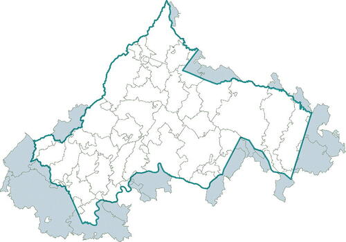
Table 1 The 14 features along with their transformations. All features except for Population_Density, Median_HH_Inc, and Mean_HH_Inc reflect the percent of population.

Feature	Transformation
Population Density (Population_Density)	Log
Age: Child (Age_Child_Pct)	Sqrt
Age: Adult (Age_Adult_Pct)	None
Age: Retired (Age_Retired_Pct)	Sqrt
Income: Less than $25,000 (Inc_Cat0_Pct)	Sqrt
Income: $25,000 to $100,000 (Inc_Cat1_Pct)	Log
Income: Greater than $100,000 (Inc_Cat2_Pct)	None
Income: Median Household (Median_HH_Inc)	None
Income: Mean Household (Mean_HH_Inc)	Sqrt
Educational Attainment (Bachelor_Plus_Pct)	Sqrt
Race: White (White_Pct)	None
Race: Black (Black_Pct)	Sqrt
Race: Asian (Asian_Pct)	Sqrt
Race: Hispanic (Hispanic_Pct)	Sqrt

2.1.1 Feature Selection

After discussion with the director of the TJHD and consulting the relevant literature, we selected the following five attributes to form strata of relatively homogeneous ZCTAs as they are (a) related to obesity and (b) available by ZCTA:

1. Population density (ACS S0101). The ZCTA population density is number of persons (all ages) divided by ZCTA area. Zhao and Kaestner (2010) look at how population density affects the BMI and obesity of residents in metropolitan areas in the U.S. and find “a negative association between population density and obesity.”

2. Age (ACS S0101). For each ZCTA the percentage of the population in these three age categories:

   1. Child: Individuals under 20 years of age.

   2. Adult: Individuals between 20 and 64 years of age.

   3. Retired: Individuals 65 years of age and older.

In their analysis of National Health and Nutrition Examination Survey (NHANES) data, Flegal et al. (2010) found that the prevalence of obesity varied by age group for both men and women.

1. Income (ACS S1901).

   1. For each ZCTA the percentage of households that fell in each of these three income categories:

      1. Less than $25,000

      2. $25,000 to $100,000

      3. Greater than $100,000

   2. ACS-reported median household income for households in each ZCTA.

   3. ACS-reported mean household income for households in each ZCTA.

Levine (2011) provided a discussion of poverty and obesity in the United States and finds that “people in America who live in the most poverty-dense counties are those most prone to obesity. Counties with poverty rates of >35% have obesity rates 145% greater than wealthy counties.” The systematic review and meta-analysis by Kim and von dem Knesebeck (2018) found that “lower income is associated with subsequent obesity (OR 1.27, 95% CI: 1.10 to 1.47; risk ratio 1.52, 95% CI: 1.08 to 2.13), though the statistical significance vanished once adjusted for publication bias.” Finally, in their analysis of neighborhood-level data from the 1990–1994 National Health Interview Survey data, Boardman et al. (2005) found that “poor areas were three times more likely than nonpoor areas to have obesity rates that exceeded 25 percent.”

1. Educational Attainment (ACS S1501): percentage of the population in each ZCTA with a bachelor’s degree or higher. The systematic review by Cohen et al. (2013) finds that

the relationship between measures of socioeconomic status like educational attainment and obesity depends on the country’s level of development, such that inverse associations are more common in more developed countries and positive associations are more common in less developed countries.

In addition, the CDC “Childhood Obesity Facts”² states that “in 2011–2014, among children and adolescents aged 2–19 years, the prevalence of obesity decreased as the head of household’s level of education increased.”

1. Race (ACS B03002). For each ZCTA the percentage of the population that identifies as “Non-Hispanic–White Alone,” “Non-Hispanic—Black Alone,” “Non-Hispanic—Asian Alone,” and “Hispanic.” In their analysis of longitudinal NHANES data, Cossrow and Falkner (2004) found that “the rise in obesity rates in women has been greatest in African-American women, followed by Hispanic women, then white women” and that “similar trends were observed in men.”

Data for all attributes come from the 2016 American Community Survey (ACS) 5-year estimates (the table names are referenced in parentheses following each attribute listed). The 5 attributes give rise to 14 features used in the analysis (see Table 1). ZCTA 22904 and 24581 had null entries for Median_HH_Inc while ZCTA 24581 had a null entry for Mean_HH_Inc. The null values were replaced with the median value for each respective feature. Because the distribution of “household income” is likely to be very skewed, the median (3(b)) will be a better summary of typical household income, while the mean (3(c)) will be more related to the total income in the area (when multiplied by the number of households).

Histograms and qq-plots were useful for indicating transformations for skewed feature distributions. Often a square root or logarithmic transformation succeeded in symmetrizing the highly skewed distributions for some features. The third column of Table 1 indicates the transformation chosen (none, square root, and log) for each feature. After transforming each feature as detailed in Table 1, pairwise plots and standard Pearson correlation coefficients were used to identify those features that were highly correlated with each other, specifically a correlation coefficient with absolute value greater than 0.75. ZCTAs 22904 and 24581 showed up as outliers: ZIP Code 22904, the ZIP Code for the University of Virginia which includes many student dormitories, maps to ZCTA 22904, so the percentage of its population that falls in the “Age: Child” category (“Individuals under 20 years of age”) is abnormally high (72.5%), and ZCTA 24581 has an extremely small population (approximately 33 people) consisting primarily of seniors. Given the outlier status of each ZCTA, ZCTAs 22904 and 24581 likely would end up as two strata each containing the single ZCTA. The UVA student body is transient and not the primary concern of the TJHD, thus ZCTA 22904 was excluded from the stratification. It would be unwise to try to sample a stratum with just 33 people, so ZCTA 24581 also was excluded from the stratification. Note that any ZCTA excluded from the stratification is also excluded from the survey.

Among the 49 remaining ZCTAs, we observed very high Pearson correlation coefficients between Inc_Cat2_Pct and Median_HH_Inc (0.79), Inc_Cat2_Pct and Mean_HH_Inc (0.90), Median_HH_Inc and Mean_HH_Inc (0.81), and White_Pct and Black_Pct (-0.76). Accordingly, White_Pct was dropped due to the high negative correlation with Black_Pct, and both Median_HH_Inc and Mean_HH_Inc were dropped due to their high correlations with Inc_Cat2_Pct. The ZCTA strata were based on the remaining 11 features.

2.1.2 Allocation Factor Analysis to Align the TJHD and ZCTA Boundaries

Figure 1 shows the boundaries of the TJHD as a wider dark blue line on top of the 51 ZCTAs that belong, in whole or in part, to the health district. The parts of the ZCTAs which lie outside the TJHD boundary are colored gray. Figure 1 illustrates that, while most of the 51 ZCTAs lie fully inside the health district boundaries, several ZCTAs have large proportions of their areas outside the health district boundary, primarily in the southwest and southeast regions of the health district.

The fact that a large proportion of a ZCTA lies outside the health district boundary does not necessarily mean that a large proportion of the ZCTA’s population also resides outside the health district. For each ZCTA that does not lie fully within the TJHD boundary, the proportion of the ZCTA population that resides inside the TJHD boundary was used to justify including the ZCTA in the stratification analysis. In this case “a sufficient population” was defined as having more than 20% of the ZCTA population residing in the TJHD. An analysis of allocation factors (see the following paragraph) for each ZCTA was used to answer this question.

The Geographic Correspondence Engine (Geocorr 2014) can show “the relationships between a wide variety of geographic coverages for the United States.” For each ZIP/county intersection Geocorr 2014 can indicate “what the size of that intersection is and what portion of the ZIP’s total population is in that intersection” (Missouri Census Data Center). For this application, the allocation factor for a ZCTA – an absolute measure of the size of the relationship between the ZCTA and the TJHD – represents the proportion of the ZCTA’s population that is located within the TJHD.³ The TJHD included 23 ZCTAs whose allocation factors (see Table C.1 in the supplementary material) fall below 1; that is, in these ZCTAs, at least one housing unit lies outside the TJHD boundary. Because ZCTAs 22952 and 24483 have 0% allocation to the TJHD and ZCTAs 23015, 24521, 23192, 23102, and 23038, all have 20% or less allocation to the TJHD, they were dropped from the analysis.

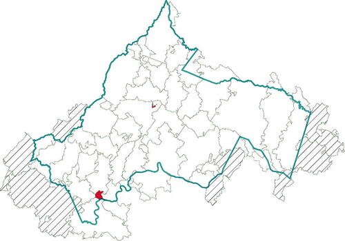
Figure 2 depicts the 9 ZCTAs excluded from the analysis: 22904 (mostly UVA students) and 24581 (only 33 residents) colored solid red, and the 7 ZCTAs with less than 20% of their housing units within the TJHD shaded with diagonal lines. These 9 excluded ZCTAs represent just 0.6% of the housing units in the TJHD, leaving 42 ZCTAs for stratification.

Fig. 2 Map showing the 9 ZCTAs that were excluded from the stratification analysis. ZCTAs 24581 and 22904 (colored solid red) were excluded due to their unusual populations for our purposes (only 33 people and transient student population, respectively). ZCTAs 22952, 24483, 23015, 24521, 23192, 23102, and 23038 (shaded with diagonal lines) were excluded following the allocation factor analysis which identified them as ZCTAs with allocations factors $\le 0.200$.

2.1.3 Hierarchical Clustering to Stratify the ZCTAs

We implemented hierarchical clustering to stratify the reduced set of 42 ZCTAs using the 11 features discussed in Section 2.1.1.⁴ A Euclidean distance cutoff of 6.25 between vectors of (standardized) features resulted in 8 strata as shown in the dendrogram in Figure 3, which indicates the different strata as using different color branches. The height of a branch point, here measured as Euclidean distance, visually depicts the similarity between one ZCTA and another, across the 11 features. The greater the height, the greater the difference; for example, the dendrogram indicates that ZCTAs 22942 and 23024 are the most similar. The purpose of the hierarchical clustering is to create ZCTA strata that are similar on the 11 features, so that a sample of households from a single stratum should yield an estimate of the obesity rate for all ZCTAs in that stratum. Geographic contiguity is not a factor. Hence, ZCTAs within a stratum may not be contiguous; see Figure 4. Irrespective of geography, the obesity rates for all ZCTAs within a stratum should be more similar than those in ZCTAs from different strata.

Fig. 3 Dendrogram of the 8 strata found using hierarchical clustering. The dendrogram branch colors indicate ZCTA stratum membership and match the colors used in the top map in Figure 4. The color bar to the immediate right of the dendrogram is another representation of ZCTA stratum membership for the 8 strata determined via hierarchical clustering and is provided to facilitate the understanding of the manual split which lead to 12 strata (shown as the color bar on the right hand side of the figure indicating ZCTA stratum membership for the 12 strata after both stratum 4 and stratum 6 were manually split into 3 strata each: 4a, 4b, 4c; 6a, 6b, 6c). The colors in the rightmost color bar match the colors used in the bottom map in Figure 4 which shows the 12 strata following the manual split.

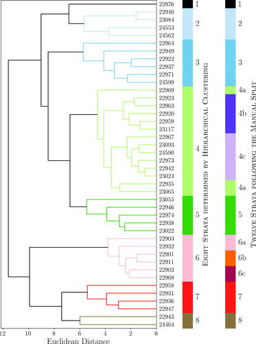
Fig. 4 Top: Map of the 8 strata determined by hierarchical clustering. The colors indicate ZCTA stratum membership and match the branch colors of the dendrogram and color bar to the immediate right of the dendrogram in Figure 3. Bottom: Map of the 12 strata which result after manually splitting 2 of the 8 strata identified by hierarchical clustering. The colors indicate ZCTA stratum membership and match the rightmost color bar in Figure 3.

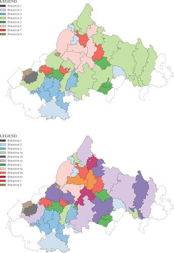
Table 2 presents the number of ZCTAs, household count, and population in each stratum. Table 2 shows that strata 4 and 6 had many more households than the other six strata (1, 2, 3, 5, 7, and 8). The results of the stratification will influence the sampling design for the survey, and having a large variance in the number of households across the different strata will require the use of more extreme weights with the survey results. Thus, we split each of the two largest of the eight strata into three parts: stratum 4 was split into 4a, 4b, and 4c while stratum 6 was split into 6a, 6b, and 6c. This decision was informed in part by the splits in the dendrogram shown in Figure 3, where we prioritized keeping together those ZCTAs indicated by the dendrogram as most similar (ZCTAs with the smallest Euclidean Distance between them), and in part by our knowledge of the region (e.g., stratum 6 was composed of the following 6 ZCTAs: 22903 and 22932 encompass UVA and immediately west of UVA; 22901 and 22911 are residential areas areas north and east of UVA; and 22902 and 22968 are two more distant and more rural areas around UVA). The manual split resulted in 12 strata, depicted in the rightmost labeled color bar in Figure 3 and in the bottom map shown in Figure 4. The stratum statistics are shown in Table 3, where the “Number of Households” column shows that this new 12-strata stratification greatly reduced the variance of the number of households across the strata.

Table 2 Stratum statistics for the 8 strata identified by hierarchical clustering. Household count and population estimates come from the 2016 ACS 5-year estimates.

Stratum ID	Color	ZCTA Count	Household Count	Population
1		1	308	621
2		4	2,543	5,473
3		6	3,805	7,491
4		14	40,478	83,746
5		5	3,740	10,715
6		6	58,029	132,263
7		4	7,217	11,440
8		2	367	531

Table 3 Stratum statistics for the 12 strata that result after manually splitting the eight strata identified by hierarchical clustering. Household count and population estimates come from the 2016 ACS 5-year estimates.

Stratum ID	Color	ZCTA Count	Household Count	Population
1		1	308	621
2		4	2,543	5,473
3		6	3,805	7,491
4a		3	1,776	3,852
4b		5	16,735	33,846
4c		6	21,967	46,048
5		5	3,740	10,715
6a		2	19,908	47,590
6b		2	23,359	51,102
6c		2	14,762	33,571
7		4	7,217	11,440
8		2	367	531

This final stratification of the 42 ZCTAs into 12 strata was used for the survey.

2.2 Survey Design

The TJHD commissioned the Center for Survey Research (CSR) at the University of Virginia to administer a mail survey to a random sample of households within the ZCTA strata. Any household within the 42 ZCTAs identified in Section 2.1.2 was eligible for selection. A household member who was at least 18 years of age was asked to complete the survey (although they could “decline to take part in the survey or skip any questions [they did] not wish to answer”). For our purposes, the survey requested information related to obesity (e.g., height, weight, gender, and age) for all household members. Although the survey needed only limited data (gender, age, height, weight for each household member) to answer the research question that motivated it (i.e., estimate obesity prevalence at the ZCTA level), these questions were part of a larger district-wide community health survey (10+ pages, 40+ questions), that aimed to “to understand the health and health priorities of residents in the Thomas Jefferson Health District (Albemarle, Fluvanna, Greene, Louisa and Nelson counties, and the City of Charlottesville) and some nearby areas.” Consequently, the sampling design of the survey had to balance the needs of this research, where estimates of the prevalence of obesity at the ZCTA stratum level are the primary concern, with the needs of the larger survey, which sought to estimate several measures at the city/county and health district level. Several factors which are correlated with obesity, including the factors used in the stratification of the ZCTAs, were collected as part of the survey.

2.2.1 Sampling Rates

Power allocation (Bankier 1988) was used to determine sampling rates, where Bankier’s equation (2.2) was used with q = 0.5 and the assumption that the (unknown) coefficients of variation for obesity were equal across all strata, in which case the S_h and ${\overline{Y}}_h$ terms drop out of Bankier’s equation (2.2) and the number of surveys allocated to stratum h is(1) $$n_h=n\frac{X_h^q}{\sum _h{X}_h^q}=n\frac{\sqrt{X_h}}{\sum _h\sqrt{X_h}}$$(1) where n is the total number of surveys and X_h is the “measure of size or importance of stratum h” (Bankier 1988), in this case the number of households in stratum h. The assumption of equal coefficients of variation across strata was made because (a) we had no prior information on within-stratum variance of obesity (BMI), and (b) responses on survey questions had unknown (probably different) variances, within and across strata. Thus, the sampling plan was stratification with sampling rates proportional to the square root of the number of households.

Table 4 shows the sampling rate for each stratum. The TJHD budget set the total number of surveys at 3005. The smallest two strata were ignored when using Equation (1)(1) $$n_h=n\frac{X_h^q}{\sum _h{X}_h^q}=n\frac{\sqrt{X_h}}{\sum _h\sqrt{X_h}}$$(1) to determine n_h as there was concern that doing so would lead to the largest clusters having extreme weights. This concern stems from the fact that the sampling objective is to balance, under a fixed cost, the need to create stratum-level estimates of the prevalence of obesity with the need to create district-level estimates for the other questions of interest to the TJHD. Thus, we set the number of addresses to sample in strata 1 and 8 at 100 each, so we would receive a sufficient number of completed surveys from each stratum (based on the past completion rates of 30% from surveys in this area, see Discussion), leading to $n=$ 2805 (3005– 200) in Equation (1)(1) $$n_h=n\frac{X_h^q}{\sum _h{X}_h^q}=n\frac{\sqrt{X_h}}{\sum _h\sqrt{X_h}}$$(1) . The “Sampling Rate” column of Table 4 is the percentage of households in a stratum that received a survey.

Table 4 Survey design and sampling rate where the strata are ordered by Household Count. Note that the number of addresses to sample in each stratum is determined by power allocation (see Equation (1)(1) $$n_h=n\frac{X_h^q}{\sum _h{X}_h^q}=n\frac{\sqrt{X_h}}{\sum _h\sqrt{X_h}}$$(1) ), except for stratum 1 and stratum 8, which are fixed at 100 each. Household counts come from the 2016 ACS 5-year estimates.

Stratum  ID	Household Count (Xh)	Addresses to Sample (nh)	Sampling Rate	Stratum Returns	Base Weight ($X_h/n_h$)
6b	23,359	432	1.8%	160 (37%)	54.07
4c	21,967	419	1.9%	131 (31%)	52.43
6a	19,908	398	2.0%	124 (31%)	50.02
4b	16,735	365	2.2%	112 (31%)	45.85
6c	14,762	343	2.3%	105 (31%)	43.04
7	7,217	240	3.3%	105 (44%)	30.07
3	3,805	174	4.6%	49 (28%)	21.87
5	3,740	173	4.6%	47 (27%)	21.62
2	2,543	142	5.6%	31 (22%)	17.91
4a	1,776	119	6.7%	36 (30%)	14.92
8	367	100	27.2%	24 (24%)	3.67
1	308	100	32.5%	26 (26%)	3.08
Overall	116,487	3,005	2.6%	950 (32%)

As mentioned in Section 2.1.3, part of the motivation for splitting the two largest strata (strata 4 and 6) of the original 8 strata suggested by the hierarchical clustering was to reduce the differences in the numbers of households across the strata, which would lead to less extreme weights in the final sample (the weights are a function of the sampling rate for each stratum); see Table 4.

2.2.2 Sample Weights

Of the 3005 surveys distributed, 1010 were returned, 950 of which could be linked to a specific stratum. The number of surveys returned by stratum can be found in the “Stratum Returns” column of Table 4. The following under- and over-representation (non-response bias) was observed to varying degrees at the district (all ZCTAs) and stratum levels in the survey data:

1. under-representation of non-White respondents,

2. slight under-representation of Hispanic/Latinx respondents,

3. slight over-representation of higher income respondents,

4. over-representation of homeowners compared to renters, and

5. over-representation of 2-person households.

The weights to account for this non-response bias were estimated via iterative proportional fitting (IPF), also called “raking” (Kalton and Flores-Cervantes 2003; Kolenikov 2014); the anesrake package in R (Pasek 2018) was used for the IPF. We chose the following factors as candidate variables in the IPF, because they addressed the over- and under-representation in the survey data, and because they were deemed important to TJHD health officers⁵:

1. Household income (S1901)

2. Hispanic ethnicity (P11, from the 2010 Census)

3. Race by household ownership (B25003A-G)

4. Household size (S2501)

5. Race (DP05)

The base weight (design weight) for stratum h was computed as $X_h/n_h$ (see the “Base Weight” column of Table 4). We used IPF to generate a set of “raked” weights for estimating at the district (all ZCTAs) level, and a different set of “raked” weights for estimating at the ZCTA-stratum level. For the former, the population marginals were computed using data from all of the ZCTAs. For the latter, the population marginals for a given stratum would typically be computed using data from ZCTAs in that stratum. Due to the low number of responses (< 50 each) in half of the 12 strata (1, 2, 3, 4a, 5, and 8), we pooled the responses for the IPF as follows: Group A consisted of strata 1, 2, 3, and 5; Group B consisted of strata 4a and 4c; Group C consisted of strata 7 and 8; and Groups D–G each consisted of a single stratum 4b, 6a, 6b, and 6c, respectively. The dendrogram in Figure 3 once again informed these groups by highlighting which strata were “closest” to each other. The population marginals for a given IPF group (A–G) were computed using data from all of the ZCTAs in that IPF group; we applied the IPF procedure separately to each Group. We note the potential for bias in Group C, which pooled the stratum with the highest response rate (stratum 7) with the stratum with the lowest response rate (stratum 8). Stratum 7 has responses from 1 in 70 households, while stratum 8 has responses from 1 in 15 households due to the oversampling. Thus, the hope is that the reduction in variance from this pooling will offset potential for bias in Group C.

Battaglia et al. (2004), Battaglia, Hoaglin, and Frankel (2009), Kolenikov (2016), and Royal (2019) described in detail the practical considerations when conducting IPF, including selection of attributes for IPF and guidelines for choosing the categories for each variable used in the process.

2.3 BMI Computation and Classification

The survey included questions regarding the gender, age, weight, and height of household members. The weight and height are required when calculating the Body Mass Index (BMI) of an individual, and BMI classification depends on gender and age for children, so this information was also solicited.

Although BMI is not a direct measure of body fat, it is viewed as strongly associated with various metabolic and disease outcomes as more direct measures of body fatness (Centers for Disease Control and Prevention 2018b). BMI is computed as $703*w/h^2$ where w is the individual’s weight in pounds and h is the height in inches.

For the purposes of BMI classification, the Centers for Disease Control and Prevention (CDC) defines an adult as an individual who is 20 years of age or older and defines a child as an individual who is at least 2 years of age and less than 20 years of age. In adults, the BMI value is used to determine the classification (see Table 5). In children, an age- and gender-specific formula is used to compute the percentile of the BMI value (Centers for Disease Control and Prevention 2018c); the BMI percentile is then used for classification purposes.

Table 5 The Centers for Disease Control and Prevention BMI classification for adults and children.

Adult	Child	Classification
BMI < 18.5	BMI Percentile < 5.0%	Underweight
18.5 $\le$ BMI < 25.0	5.0% $\le$ BMI Percentile < 85.0%	Healthy Weight
25.0 $\le$ BMI < 30.0	85.0% $\le$ BMI Percentile < 97.5%	Overweight
30.0 $\le$ BMI	97.5% $\le$ BMI Percentile	Obese

3 Results

The data from the survey were analyzed using the survey package in R (Lumley 2020, 2004) at two different spatial resolutions: the ZCTA stratum and the district as a whole (all ZCTAs).

Figure 5 displays maps of the prevalence of obesity by ZCTA stratum for adults (top) and children (bottom), where the color of the ZCTA encodes the prevalence of obesity. Table 6 gives the point estimates of the prevalence of obesity along with the uncertainty in the estimate in the form of margin of error (MOE), the half-width of a 95% confidence interval. The survey package uses Taylor Series linearization (see Lumley 2010, sec. A.2) to generate standard errors and MOEs. The survey package will not generate a standard error or MOE if the prevalence estimate is equal to 0.0% or 100%. Tables D.1 to D.3 in the supplementary material contain the point estimates and associated MOEs for the underweight, healthy weight, and overweight classifications, respectively.

Fig. 5 Maps showing prevalence of obesity by ZCTA for adults (top) and children (bottom).

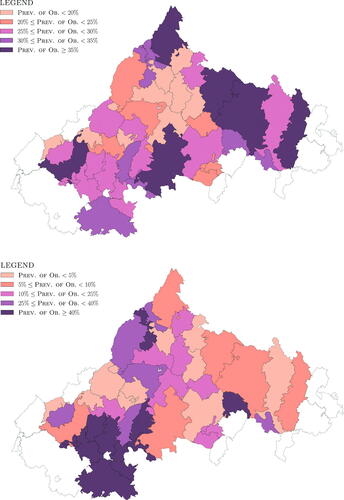
Table 6 Point estimates and margin of error (MOE, the half-width of the 95% confidence interval) for the prevalence of obesity and the number of individuals in the population classified as obese by ZCTA stratum for both adults and children. The final row presents the prevalence of obesity and the number of individuals in the population classified as obese across the entire district (all ZCTAs).

	Prev. of Obesity (MOE)				No. Obese (MOE)
Stratum ID	Adult		Child		Adult		Child
1	29.8%	(14.2%)	35.2%	(28.3%)	104	(49)	95	(76)
2	32.5%	(17.9%)	43.2%	(60.7%)	1,305	(717)	629	(883)
3	25.6%	(10.4%)	41.8%	(25.9%)	1,470	(597)	730	(452)
4a	34.0%	(17.7%)	37.0%	(47.0%)	983	(512)	357	(455)
4b	29.4%	(8.8%)	2.6%	(5.5%)	7,938	(2,364)	176	(379)
4c	36.3%	(9.3%)	8.4%	(10.3%)	12,754	(3,269)	924	(1,128)
5	23.6%	(11.1%)	12.8%	(15.8%)	1,887	(888)	346	(426)
6a	21.6%	(6.3%)	25.3%	(18.1%)	7,994	(2,325)	2,661	(1,907)
6b	16.9%	(5.7%)	12.7%	(9.0%)	6,585	(2,245)	1,531	(1,087)
6c	18.7%	(7.9%)	20.9%	(14.6%)	4,850	(2,043)	1,585	(1,101)
7	15.1%	(6.0%)	0.0%	(–)	1,408	(562)	0	(–)
8	9.6%	(11.4%)	0.0%	(–)	47	(56)	0	(–)
All ZCTAs	26.0%	(3.4%)	19.5%	(6.4%)	50,810	(6,539)	11,172	(3,651)

Given the MOE in Table 6, it is not possible to test differences across specific strata, but the results presented in Table 6 and displayed in Figure 5 indicate clear differences and a wide spread in the prevalence of obesity across the 12 strata in the TJHD, for both adults and children. The differences suggest that, if addressing obesity is important to decision makers in the TJHD, then using the single, district-wide estimate of the prevalence of obesity from the BRFSS will not suffice for targeting resources where they are most needed. Columns 4 and 5 of Table 6 show the point estimate (with MOE) for the number of people classified as obese. The information in columns 4 and 5 of Table 6 is important to public health officials because it allows them to identify ZCTAs with a large number of obese people, rather than just ZCTAs with a high prevalence of obesity. For example, ZCTA 22968 (part of stratum 6a) has an estimated adult prevalence of obesity of 21.6% and a 2018 census of 7935 adults, resulting in an estimated 1714 obese adults in the ZCTA, while ZCTA 22969 (part of stratum 4a) has an adult prevalence of obesity of 34.0% and a 2018 census of 971 adults resulting in an estimated 330 obese adults in the ZCTA.

In Table 6, the row corresponding to stratum 7 indicates that none of the surveys had a child who was classified as obese. This is a somewhat counter-intuitive result given that 105 surveys were returned from stratum 7, and other strata with lower numbers of returned surveys have nonzero prevalence of obesity estimates. Those 105 (household) surveys from stratum 7 contained data (i.e., responses to the relevant questions) on 222 individuals which allowed us to determine 222 individual BMI classifications (see Table E.1 in the supplementary material). Of these 222 individuals only 21 fell into the “Child” age group, and none of the 21 fell into the “Obese” category. Thus, the number of returns from a stratum does not say much about the number of individuals in the “Child” age group from that stratum.

Finally, the estimated adult prevalence of obesity for the entire district (all ZCTAs), 26.0% (with MOE of 3.4%), is similar to the most recent 2014 BRFSS estimate of 27.7% (95% confidence interval of $21.3\%-34.2\%$, MOE of 6.4%) for the TJHD which appears on the Virginia Department of Health website.

4 Discussion

The research in this article was driven by the need for increased detail in the data on prevalence of obesity for a health district. The single estimate from BRFSS applies to the entire district, which was deemed too broad to be useful for local public health professionals. To address this issue, a survey was conducted with the expectation that a survey would reduce the sampling bias that might affect estimates from other administrative sources of data. For example, an estimate of obesity prevalence using measurements from patients who visited a health clinic will be biased because such patients tend to be less healthy than the general population. Moreover, due to the more “local” and trusted nature of the survey source (TJHD in cooperation with University of Virginia, versus the Federal government), a lower non-response rate was anticipated, and a larger sample size could be collected (950 versus BRFSS’s 248) that would allow obesity prevalence estimates at a much smaller spatial resolution than the currently available point estimate (district level). Because cost considerations prohibited a precise estimate of the prevalence of obesity for each individual ZCTA in the district, we stratified ZCTAs that we judged to be relatively homogeneous with respect to features associated with obesity, and the sampling could be conducted efficiently within a stratum of ZCTAs. In this article, we provided a strategy to achieve this objective, via these steps

1. choose a spatial resolution for analysis (here, ZCTA);

2. select attributes for stratifying units into strata that should be relatively homogeneous with respect to the target outcome (here, 11 features from the ACS data);

3. stratify the units (here, via hierarchical clustering);

4. design the survey; and

5. analyze the survey results (accounting for non-response, etc.).

We believe that this approach will be useful and applicable for obtaining estimates for any population-based target quantity (e.g., chronic disease prevalence, physical activity levels, vaccination or screening rates), for any area, under similar cost constraints.

As a telephone survey, the BRFSS survey relies on self-reported height and weight. Research has shown that self reports of height and weight can be unreliable (overestimation of height, underestimation of weight) (Stromel and Schoenborn 2009). Telephone surveys may be especially unreliable, as immediate answers are requested. A limitation of the TJHD survey is that, like the BRFSS survey, responses here were also self-reported. However, the TJHD survey was mailed to the respondents; they could complete it at their leisure. Thus, respondents had the opportunity to measure their height and weight before writing them down, or find them from a report as recorded in previous health visit documentation, either of which would make the TJHD survey information more reliable than that from a telephone survey. Low survey responses rates can introduce non-response bias. Based on CSR’s experience with administering surveys in the local area (which includes the TJHD), CSR expected an overall return rate of 30%, or about 900 returned surveys. The final overall response rate for the TJHD survey was 32%, close to their estimate; see Table 4. The length of the TJHD survey likely played a part in this low response rate—the survey booklet was over 10 pages long and contained over 40 questions. People who might have responded to a shorter survey may not have responded to the TJHD survey after seeing its length.⁶ We tried to address this non-response bias through IPF (see Section 2.2.2).

A limitation of this research lies in the survey design, specifically with the expected number of returned surveys in strata 1, 2, 3, 4a, 5, and 8. Assuming that CSR was correct in their estimated rate of return of 30%, the expected number of returns in the aforementioned 6 strata would be less than 55 returned surveys per stratum. That low number should have alerted us to an insufficient number of survey responses in individual strata for the IPF, and we may have considered possible changes in the survey design (see the end of Section 2.2.2).

Finally, we note that the American Community Survey (ACS) is a sample; accordingly, ACS point estimates all have uncertainties associated with them. In this research, the point estimates were used in the stratification of the ZCTAs (they were considered the best estimates of the values of interest) without accounting for this uncertainty. Indeed, the short article “Approximate Weights” by Tukey (1948) shows the increase in variance in a misweighted mean; the weights have to be off by a factor of 3 before serious variance inflation occurs. A more careful stratification approach might take account of these uncertainties, and both sets of results (without versus with incorporation) can be compared.

As noted in the introduction, the BRFSS survey was limited to adults and gave only a point estimate for the prevalence of adult obesity for the entire health district, so it was of limited use to public health officials for targeting interventions across the district. The TJHD survey data yielded the most detailed estimates to date for the prevalence of obesity for both children and adults in the TJHD, and the only estimates for the prevalence of childhood obesity in the TJHD. In addition, compared with the 248 responses used to generate the point estimate of the prevalence of obesity for the TJHD, the 950 responses from the survey allow a more precise estimate at the district level (compare the MOE of 6.4% for the 2014 estimate from the BRFSS to the MOE of 3.3% for the 2018 estimate from the TJHD survey). The survey also allowed estimation of the prevalence of underweight, healthy weight, and overweight BMI classifications. Several community agencies have used the information (both the estimates and the maps) generated by this effort. For example, the Thomas Jefferson Health District (now the Blue Ridge Health District) included the maps as part of the district Community Health Assessment. In addition, the maps were used by a local non-profit focused on food insecurity to support grant applications for funding to advance food equity. Finally, in conjunction with a local food bank, the maps were used by the health department to select a target area to expand a fresh food distribution network.

Future research will focus on estimating prevalence of obesity using Electronic Medical Record (EMR) data from patient visits to one of the primary health systems in the TJHD. This research will use the findings from the survey as benchmarks for judging whether it is possible to adjust the convenience sample of EMR data to generate reliable estimates of the prevalence of obesity in a health district. The approach we have taken is “model-free;” small area estimation models (see Rao (2003) or Pfeffermann (2002)) can possibly be used to reduce the uncertainty in the point estimates given the availability of American Community Survey data at the ZCTA level for this region. Such models will involve assumptions that would need to be verified, so we leave this avenue as the subject of future research.

Acknowledgments

We are most grateful to the editor and the anonymous reviewers whose comments greatly improved our article. We also thank Barry Graubard (National Cancer Institute) for advice on the analysis, and Thomas Guterbock and Kara Fitzgibbon (Center for Survey Research, University of Virginia) for assistance with survey questions.

Competing interests: BL reports research support from Dexcom, Inc. handled by the University of Virginia, and royalties from Dexcom, Inc. handled by the University of Virginia’s Licensing and Ventures Group.

Ethical approval: Collection and subsequent analysis of the data from the survey was performed under the University of Virginia’s Social and Behavioral Sciences IRB protocol number 2018025900.

Supplementary Material

The supplementary material contains a map showing the TJHD ZCTAs, prevalence estimates for Underweight, Healthy Weight, and Overweight, and some survey statistics. Some analysis code and data can be found at https://github.com/bjl2n/tjhd_prevalence_of_obesity.

Additional information

Funding

BL acknowledges support in part from an internal grant from the University of Virginia’s Translational Health Research Institute of Virginia (THRIV). KK acknowledges support in part from the National Center For Advancing Translational Sciences of the National Institutes of Health (NIH) under Award Number UL1TR003015. Authors are solely responsible for the content which does not represent the official views of the NIH.

Notes

1 In 2021 the Thomas Jefferson Health District was renamed the Blue Ridge Health District (BRHD).

2 www.cdc.gov/obesity/data/childhood.html.

3 Geocorr 2014 is located at mcdc.missouri.edu/applications/geocorr2014.html. To generate the correlation list for the research in this article, under Input Options:

“Virginia” was selected as the State.

“2010 Geographies: ZIP/ZCTA” was selected as the Source Geography.

“2014 Geographies: County” was selected as the Target Geography.

“Housing Units (2010 census)” was selected as the Weighting Variable.

Housing units (www.census.gov/housing/hvs/definitions.pdf) were used as a proxy for the population of the ZCTA because the survey was mailed to randomly selected addresses (where an address corresponds to a housing unit).

4 Because the ranges vary greatly for these 11 features, they were first scaled using the scale function of the sklearn.preprocessing Python library (Pedregosa et al. 2011). The scipy.cluster.hierarchy Python module (Oliphant 2007; Millman and Aivazis 2011) implementation of hierarchical clustering with the Ward variance minimization algorithm was used to calculate Euclidean distances between the strata.

5 Unless otherwise noted the labels in parentheses refer to the American Community Survey 2016 5-year estimate data tables from which population totals were taken.

6 We raised the adverse consequences of a long survey during the planning stages. The survey length arose from other units in the public health department who desired additional information beyond simply estimates of the prevalence of obesity.

References

- Bankier, M. (1988), “Power Allocations: Determining Sample Sizes for Subnational Areas,” The American Statistician, 42, 174–177.
- Battaglia, M., Hoaglin, D., and Frankel, M. (2009), “Practical Considerations in Raking Survey Data,” Survey Practice, 2, SP–2009–0019. DOI: 10.29115/SP-2009-0019.
- Battaglia, M., Izrael, D., Hoaglin, D., and Frankel, M. (2004), “Tips and Tricks for Raking Survey Data (a.k.a. Sample Balancing),” in Proc. 59th Annual Conference of the American Association for Public Opinion Research (Phoenix, AZ, May 2004), pp. 4740–4745.
- Boardman, J., Saint Onge, J., Rogers, R., and Denney, J. (2005), “Race Differentials in Obesity: The Impact of Place,” Journal of Health and Social Behavior, 46, 229–243. DOI: 10.1177/002214650504600302.
- Centers for Disease Control and Prevention. (2018a), “CDC National Health Report Highlights.” Available at www.cdc.gov/healthreport/publications/compendium.pdf.
- Centers for Disease Control and Prevention (2018b), “Healthy Weight—About Adult BMI.” Available at www.cdc.gov/healthyweight/assessing/bmi/adult_bmi/index.html.
- Centers for Disease Control and Prevention (2018c), “Percentile Data Files with LMS Values.” Available at www.cdc.gov/growthcharts/percentile_data_files.htm, Last accessed on 2018-09-14.
- Centers for Disease Control and Prevention (2021), “Why It Matters - Obesity is Common, Serious, and Costly.” Available at www.cdc.gov/obesity/about-obesity/why-it-matters.html.
- Cochran, W. (1977). Sampling Techniques (3rd ed.), John Wiley & Sons.
- Cohen, A., Rai, M., Rehkopf, D., and Abrams, B. (2013), “Educational Attainment and Obesity: A Systematic Review,” Obesity Reviews, 14, 989–1005. DOI: 10.1111/obr.12062.
- Cossrow, N., and Falkner, B. (2004), “Race/Ethnic Issues in Obesity and Obesity-Related Comorbidities,” The Journal of Clinical Endocrinology & Metabolism, 89, 2590–2594.
- Flegal, K., Carroll, M., Ogden, C., and Curtin, L. (2010), “Prevalence and Trends in Obesity Among Us Adults, 1999–2008,” Journal of the American Medical Association, 303, 235–241. DOI: 10.1001/jama.2009.2014.
- Ghosh-Dastidar, B., Cohen, D., Hunter, G., Zenk, S., Huang, C., Beckman, R., and Dubowitz, T. (2014), “Distance to Store, Food Prices, and Obesity in Urban Food Deserts,” American Journal of Preventive Medicine, 47, 587–595. DOI: 10.1016/j.amepre.2014.07.005.
- Kalton, G., and Flores-Cervantes, I. (2003), “Weighting Methods,” Journal of Official Statistics, 19, 81–97.
- Kim, T., and von dem Knesebeck, O. (2018), “Income and Obesity: What Is the Direction of the Relationship? A Systematic Review and Meta-Analysis,” BMJ Open, 8, e019862.
- Kolenikov, S. (2014), “Calibrating Survey Data Using Iterative Proportional Fitting (Raking),” The Stata Journal, 14, 22–59. DOI: 10.1177/1536867X1401400104.
- Kolenikov, S. (2016), “Post-Stratification or Non-Response Adjustment?” Survey Practice, 9, SP–2016–0014.
- Levine, J. (2011), “Poverty and Obesity in the U.S.” Diabetes, 60, 2667–2668. DOI: 10.2337/db11-1118.
- Lumley, T. (2004), “Analysis of Complex Survey Samples,” Journal of Statistical Software, 9, 1–19. R package version 2.2.
- Lumley, T. (2010), Complex Surveys: A Guide to Analysis Using R: A Guide to Analysis Using R. John Wiley and Sons.
- Lumley, T. (2020), “survey: Analysis of Complex Survey Samples.” R package version 4.0.
- Millman, K., and Aivazis, M. (2011), “Python for Scientists and Engineers,” Computing in Science Engineering, 13, 9–12. DOI: 10.1109/MCSE.2011.36.
- Missouri Census Data Center. (2021), “Geocorr 2014: Geographic Correspondence Engine.” Available at mcdc.missouri.edu/applications/geocorr2014.html.
- National Association of County and City Health Officials. (2021), “Mobilizing for Action Through Planning and Partnerships (MAPP).” Available at www.naccho.org/programs/public-health-infrastructure/performance-improvement/community-health-assessment/mapp.
- Oliphant, T. (2007), “Python for Scientific Computing,” Computing in Science Engineering, 9, 10–20. DOI: 10.1109/MCSE.2007.58.
- Pasek, J. (2018), “anesrake: Anes Raking Implementation,” R package version 0.80.
- Pedregosa, F., Varoquaux, G., Gramfort, A., Michel, V., Thirion, B., Grisel, O., Blondel, M., Prettenhofer, P., Weiss, R., Dubourg, V., Vanderplas, J., Passos, A., Cournapeau, D., Brucher, M., Perrot, M., and Duchesnay, E. (2011), “Scikit-Learn: Machine Learning in Python,” Journal of Machine Learning Research, 12, 2825–2830.
- Pfeffermann, D. (2002), “Small Area Estimation-New Developments and Directions,” International Statistical Review, 70, 125–143.
- Rao, J. (2003). Small Area Estimation (1st ed.), Hoboken, NJ: Wiley.
- Royal, K. (2019), “Survey Research Methods: A Guide for Creating Post-Stratification Weights to Correct for Sample Bias,” Education in the Health Professions, 2, 48–50. DOI: 10.4103/EHP.EHP_8_19.
- Stromel, M., and Schoenborn, C. (2009), “Accuracy and Usefulness of BMI Measures on Self-Reported Weight and Height: Findings From the NHANES and NHIS 2001–2006,” BMC Public Health, 9, 421. DOI: 10.1186/1471-2458-9-421.
- Tukey, J. (1948), “Approximate Weights,” Annals of Mathematical Statistics, 19, 91–92. DOI: 10.1214/aoms/1177730297.
- UDS Mapper. (2018), “ZIP Code to ZCTA Crosswalk.” Available at udsmapper.org/zip-code-to-zcta-crosswalk/.
- U.S. Census Bureau. (2018), “ZIP Code Tabulation Areas.” Available at www.census.gov/geo/reference/zctas.html.
- VCU Center on Society and Health. (2018), “Mapping Life Expectancy.” Available at societyhealth.vcu.edu/work/the-projects/mapping-life-expectancy.html.
- Virginia Department of Health. (2018), “Behavioral Risk Factor Surveillance Survey—Data.” Available at www.vdh.virginia.gov/brfss/data/#OBESITY.
- Virginia Planning District 10, Thomas Jefferson Health District. (2016), “MAPP2Health.” Available at www.vdh.virginia.gov/content/uploads/sites/91/2016/07/MAPP2HealthFinalSmall.pdf.
- Zhao, Z., and Kaestner, R. (2010), “Effects of Urban Sprawl on Obesity,” Journal of Health Economics, 29, 779–787. DOI: 10.1016/j.jhealeco.2010.07.006.