Changes in Crime Rates during the COVID-19 Pandemic

Abstract

We estimate changes in the rates of five FBI Part 1 crimes during the 2020 spring COVID-19 pandemic lockdown period and the period after the killing of George Floyd through December 2020. We use weekly crime rate data from 28 of the 70 largest cities in the United States from January 2018 to December 2020. Homicide rates were higher throughout 2020, including during early 2020 prior to March lockdowns. Auto thefts increased significantly during the summer and remainder of 2020. In contrast, robbery and larceny significantly declined during all three post-pandemic periods. Point estimates of burglary rates pointed to a decline for all four periods of 2020, but only the pre-pandemic period was statistically significant. We construct a city-level openness index to examine whether the degree of openness just prior to and during the lockdowns was associated with changing crime rates. Larceny and robbery rates both had a positive and significant association with the openness index implying lockdown restrictions reduced offense rates whereas the other three crime types had no detectable association. While opportunity theory is a tempting post hoc explanation of some of these findings, no single crime theory provides a plausible explanation of all the results. Supplementary materials for this article are available online.

Keywords:

• COVID-19
• Crime trends
• Pandemic lockdowns
• Part 1 crimes

1 Introduction

The COVID-19 pandemic has prompted a few early analyses on the impacts of lockdowns aimed at curtailing the pandemic’s spread on crime rates. The initial lockdowns in the United States began in March 2020 and generally eased in May 2020. Another momentous event, the death of George Floyd at the hands of Minneapolis police on May 25, 2020, coincided with the easing of the lockdowns. George Floyd’s killing prompted protests across the United States which were overwhelmingly peaceful but, in some cities, involved violence or property damage by protesters or counter-protesters.

During the summer and fall of 2020, various media sources reported that homicide counts had risen in some of America’s largest cities based on year-to-date comparisons (Asher and Horwitz 2020; Hilsenrath 2020; McCarthy 2020; Struett 2020) and month-to-month comparisons (Campbell 2020) between 2020 and previous years. Meanwhile, other crimes, such as burglary and robbery, were reported to have decreased in the months following the start of the COVID-19 pandemic in the United States (Becker and Corley 2020; FBI 2020; Lopez 2020).

In this article, we report findings of an analysis of the pandemic’s impact in 28 of the 70 largest U.S. cities on five FBI Part 1 Index crimes—homicide, auto theft, burglary, robbery, and larceny. These are all of the cities that make weekly crime counts available. Concerning analyses of crime rates following George Floyd’s killing, we are not able to disentangle the underlying reasons for changes we identify, which may include social unrest, economic conditions, changed police behavior, or other factors. Our aim instead is to carefully document changes or the absence of changes accounting for seasonal trends. The patterns we document are complex: For homicide, the crime on which the most media attention has focused, seasonally-adjusted rates in 2020 were higher relative to 2018 and 2019 throughout the year including during the January and February preceding the onset of the lockdown period in March 2020 and the ensuing events following the murder of George Floyd in late May 2020. While point estimates of the increase during the summer protest and rest of year periods are larger than in the winter pre-pandemic period the differences are not statistically significant at the 0.05 level. This finding calls into question explanations for the homicide increase that attribute the increase to factors related to summer protest events following George Floyd’s killing (Graham 2021). We also identify significant increases in auto theft rates in the summer protest and end of year periods. In contrast, we detect significant declines in larceny and robbery throughout the three post-pandemic periods. For burglary, the point estimates all suggest declines throughout 2020, but only the pre-pandemic period estimate is significant at the 0.05 level.

We also conducted two detailed analyses of the impact of the spring lockdown period on crime. For these analyses, we consider data up to the week of George Floyd’s murder. One analysis was designed to detect whether crime trends changed over successive biweekly periods as the lockdown progressed. Results for robbery and larceny mirror the findings of the first regression model—both were significantly down for all biweekly lockdown periods and did not appear to vary between the start and end of the lockdown period. For the other crimes most biweekly period estimates were nonsignificant, and the few significant, larger differences tended to occur at the very start or end of the lockdown period. The second analysis examines the association of weekly crime rates with an “openness index” which we created that assigned integer values to cities each week based on the strictness of the cities’ lockdowns. We found that weekly larceny and robbery rates significantly increased in concert with the openness index implying the lockdown restrictions reduced both crime types but that the other crime types were not significantly associated with the index.

Thus, overall, we find that the COVID-19 pandemic and mass protests related to the killing of George Floyd were associated with significant changes in urban crime in the United States, but the direction of changes varies by crime type: homicides and auto thefts were up but with the caveat that homicides were up throughout 2020, not just during the pandemic periods, and robberies and larcenies were down.

Due to the recency of these events, few academic articles have been written about how crime rates have changed during pandemic-related lockdowns and following the loosening of these lockdowns in the United States. Piquero et al. (2020) analyzed how the COVID-19 lockdown in Dallas was associated with a spike in domestic violence in the two weeks after the lockdown began. Campedelli, Aziani, and Favarin (2021) also found mixed associations with the lockdown in Los Angeles and various crime rates in March 2020. Mohler et al. (2020) analyzed daily police calls-for-service data from Los Angeles and Indianapolis from a month after lockdowns went in place and used regression models to compare these months to the months of 2020 leading up to the lockdowns. They found mixed results across crimes and the two cities. Ashby (2020) used seasonal auto-regressive integrated moving average (SARIMA) models to address seasonality while determining whether certain classes of crimes are significantly different from these models’ forecasts in sixteen large U.S. cities. Each city was modeled separately, and the data coverage ended on May 10th. This early analysis found no evidence in this set of cities that serious assaults in public or in residences increased or decreased between when the first COVID-19 case was reported in the U.S. in January until May 10th. The results also suggested that changes in crime trends varied across these cities. Abrams (2020) also provided an early analysis of a variety of crime rates per capita. Using data from 23 U.S. cities, this article found that there was no statistically significant increase in homicides the four weeks after lockdowns went in place. However, Abrams (2020) found that drug crimes, violent crimes, and most property crimes declined in these four weeks in those cities.

The difference between the findings of our study and some previous analyses of homicide and other crime rates is likely attributable to several factors. First, we analyze data through December 2020 from 28 cities. Unlike other analyses, our focus was not on identifying individual cities that might have experienced increases in crime; rather it was to examine whether in a combined analysis of 28 cities there was evidence of a systematic change in various Part 1 crime rates. To our knowledge, we are the first study to consider how annual crime rates compare between the 28 cities included relative to all 70 largest cities in the United States. Furthermore, with the exception of Rosenfeld, Abt, and Lopez (2021), combined analyses of cities have not used data beyond the summer of 2020, which prevents these analyses from fully examining seasonal trends or the persistence of any crime rate changes. Second, we assembled data on the exact timing and strictness of the lockdown over time for each city during the lockdown period which allows us to include an index of openness in our analysis. Third, we focus specifically on the impact of the lockdown and subsequent opening up on crime throughout the year whereas other analyses (e.g., Coote 2020) with the exception of Rosenfeld, Abt, and Lopez (2021), focus more on the question of whether homicide in particular overall increased in 2020 including the pre-lockdown months.

Because we have data available from after initial lockdowns were relaxed throughout the summer and fall and into early winter, thus, allowing seasonal trends to be properly detected, we further contribute to previous work by illustrating how evolving policies surrounding the pandemic were associated with possible changes in crime rates. Using panel regression models, we account for seasonality as well as year-to-year changes in homicide and other crime trends across many U.S. cities. Furthermore, we are unaware of any articles besides work by Rosenfeld, Abt, and Lopez (2021) that has analyzed crime trends in multiple cities following the killing of George Floyd, which we are able to do due to our 2020 data coverage continuing throughout the entire year. Rosenfeld, Abt, and Lopez (2021) take the average of crime rates across cities (12–34 cities, median 18, depending on crime type) each month from 2017 to 2020 and treat it as a single time series. They then use time series analysis to identify “structural breaks” in the averaged crime rate during the pandemic. As described below, we retain the variability present in the full weekly panel structure of the data and use established panel regression methods to identify whether crime rates departed from prior patterns in a systematic fashion over specific periods during the pandemic.

2 Data and Methods

2.1 Data Sources

The outcome variables of interest are weekly crime counts by type of crime. We used publicly available crime incident report data from 28 of the 70 largest cities in the United States (WorldPopulationReview.com 2020). These 28 cities are those that made daily- or weekly-level data publicly available for the full years of 2018, 2019, and 2020 in an accessible and usable format. For example, four cities (Nashville, Louisville, Houston, and Seattle) in our dataset published NIBRS data, which was straightforward to categorize into crime types. Table A.1 in the supplementary materials shows which variable in each city’s data file was used to identify crime descriptions and which crime descriptions or codes for each city were classified into each of these five Part 1 crimes.

Table 1 Summary of population and crime counts and rates per 100,000 People in 2018–2019.

		Mean	Within-City SD	Between-City SD
Population	Count	1,212,684	NA	1,627,697
Homicide	Count	2.792	1.686	2.621
	Rate	0.326	0.2379	0.337
Auto Theft	Count	89.345	14.366	70.684
	Rate	10.278	1.932	6.122
Burglary	Count	106.367	16.75	75.588
	Rate	11.988	2.224	6.013
Robbery	Count	58.149	11.114	58.804
	Rate	5.517	1.330	3.781
Larceny	Count	528.278	59.432	521.227
	Rate	50.805	6.796	18.829

We examine how the cities in our study compare with all large cities in terms of annual crime rates. To determine rates per capita, we used U.S. Census Bureau Subcounty Resident Population Estimates from 2010 to 2019 (U.S. Census Bureau 2020). In Figures A.1–A.5, supplementary materials show the crime data in 2018 for each of the five crime types we analyze for the 28 cities in our analysis compared with all of the 70 most populous U.S. cities. These figures demonstrate that the distributions of annual crime rates were similar for the 28 cities included in this study to those for all 70 largest cities in 2018.

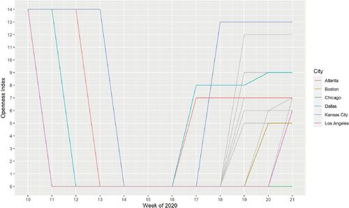
Fig. 1 Variation in the openness index during the lockdowns. Week 10 begins on March 8, 2020, and Week 21 begins on May 24, 2020.

We identified data on five of seven FBI UCR Part 1 crimes: homicide, robbery, burglary, larceny, and auto theft. The two Part 1 crime types we do not fully analyze are rape and aggravated assault. Though 26 of these cities made data about crime reports related to rape available, due to the inconsistent nature of classifying a crime as rape across cities, we decided to not include rape in our analyses. For aggravated assault, data was widely available from these cities, but the 2018 aggregated yearly totals from the weekly data were on average 20% lower than the 2018 UCR reported yearly totals, which caused us to be concerned about the quality of the weekly aggravated assault count. We believe the differences between the weekly data and the UCR data were largely due to inconsistencies about classifying crimes as “aggravated” versus less serious assault. We include results for aggravated assault in supplementary materials. Because rape and aggravated assault are both serious forms of violence, their data quality issues are unfortunate. More consistent recording of these two important crime types would be very desirable. Table A.2, supplementary materials lists the 28 cities and which analyses we included them in.

We also gathered data from media sources (CNN 2020; The New York Times 2020) and state and county health departments regarding lockdown dates for 27 of the 28 cities and the timing and strictness of pandemic-related lockdown reopening phases during the spring and summer of 2020 for 23 of the 28 cities. The cities for which we do not have lockdown dates (Milwaukee) or information about reopening phases (Milwaukee, Mesa, Raleigh, St. Paul, and Tulsa) were late additions to our analyses. Consequently, we were not able to recover the lockdown date for Milwaukee or weekly information about reopening phases at the level that would have allowed us to assign these cities weekly openness index values. From this information, we created two different measures of the lockdown stage a given city was in during a particular week. The first simply measured in two-week intervals the amount of time that has passed since the initial lockdown measure was put in place in each city. These do not align with calendar time as different cities began their lockdowns at different times. The other was a measure of the extent to which each city was open or locked down in each week which we refer to as an “openness index.” The index was on a scale from 0 (least open) to 14 (most open). For all weeks leading up to a city’s COVID-related lockdown week, this index took a value of 14. The value for the index for the weeks after a city’s lockdown were determined by how restricted certain sectors of the economy were. The sectors we considered were “Entertainment,” “Food and Drink,” “Industries,” “Outdoor and Recreation,” “Personal Care,” “Places of Worship,” and “Retail,” and each sector could be assigned a value of 0 (no components of this sector were operating at any capacity), 1 (at least some industries in the sector were not operating at full capacity), or 2 (all industries in the sector were operating at full capacity). We visualize the variation in the openness index in 2020 across all available cities in Figure A.6, supplementary materials and show some illustrative examples in Figures 1. For more information about what industries fell under each sector, please refer to Table A.3, supplementary materials.

2.2 Methods

To measure the associations between stages of the COVID-19 pandemic and crime rates, we use two different sets of Poisson regression models.¹ In all analyses, our unit of analysis is a city-week pair. The first set of models focuses in detail on the lockdown period and describes crime patterns in relation to specific pandemic-related lockdown timing and lockdown strictness compared to crime trends from the past two years. These models include 2020 data from January through week 21, the week of the killing of George Floyd, and the week before ensuing protests occurred in most cities across the United States. The second set of models tests whether seasonal crime trends over each of four periods of 2020 are significantly different from those in the past two years. This set of models includes data for all of 2020, encompassing months before the pandemic lockdowns, the spring lockdown, summer mass protests sparked by the killing of George Floyd by police in Minneapolis, and the remainder of 2020 after major protest activity ceased and the pandemic continued. We conduct post-estimation tests to determine whether the crime rates in these four periods of 2020 differ from each other. All models include an offset term for the city’s population, city fixed effects to account for different crime rates by city, and year and month fixed effects to account for seasonal and time trends. We cluster standard errors at the city-level in all of our models.

In these analyses, week units are seven days long, and we prioritized keeping approximated month units that were composed of these full week units. This results in approximate month units consisting of four or five full weeks as seen in Table A.4 in the supplementary materials.

2.2.1 Response Variable

For all models, we used the same form of the response variables, city-wide weekly crime count. For each type of crime we analyze, let $c=1,\mathrm{}\dots ,28$, r = 2018, 2019, 2020, and $w=1,\mathrm{}\dots ,52$ index the city, year, and week of the year of interest, respectively. For each crime type, the response variable is(1) $$\begin{array}{c}{y}_{\text{cwr}}={(\text{crime count})}_{\text{cwr}}\hfill \end{array}$$(1)

2.2.2 Model of Crime Rates by Openness Index

To understand how relationships between crime rates and pandemic-related lockdowns may vary over the duration of the lockdowns, we used two different types of models. For both types of models, we restricted the data to end in week 21 of 2020, the last week of May and the week in which George Floyd was killed. By this week, many cities had significantly loosened lockdown restrictions, and protests following George Floyd’s killing were occurring in a few but not yet most cities.

The first type of model focused on the relationship between crime rates and levels of city openness which varied across cities and over time. There were 2695 city-week observations for the homicide version of this model and 2818 observations for all other crime types’ models. For each crime type, weekly crime counts were modeled with city fixed effects (22 parameters, ${\zeta }_c)$, month fixed effects (11 parameters, ${\theta }_{m(w)})$, year fixed effects (2 parameters, ${\gamma }_r)$ and a linear specification of the degree of city openness (1 parameter, $\beta )$.:(2) $$\begin{array}{c}E\left(y_{\text{cwr}}\right)={\lambda }_{\text{cwr}}=f(1\ast Po{p}_c+\alpha +{\gamma }_r+{\theta }_{m\left(w\right)}+{\zeta }_c\\ \hspace{1em}+\beta \ast \text{openness}{\text{index}}_{\text{cwr}}).\end{array}$$(2)

The model contains an intercept term, α, reflecting log crime rates per week in January 2018 for the omitted city (Atlanta) and an offset term for the population size of each city, ${\text{Pop}}_c$. The year fixed effect for 2018, ${\gamma }_{2018}$, is set to zero. Months are a function of weeks as specified in Table A.4, supplementary materials, and the fixed effect for the first month, January, is set to zero. The link function for the Poisson model, $f()$, is the exponential function. On the incident rate ratio scale, the coefficient of interest, $\text{exp}\hspace{0.17em}(\beta )$, is the average multiplicative change in weekly crime count associated with a one unit increase in the openness index. Using polynomial specifications of the openness index, we assessed whether a more flexible specification of openness was needed and no clear evidence of nonlinear associations was detected.²

2.2.3 Model of Crime Rates by Weeks into Lockdown

The second model type focused on the relationship between crime rates and the progression of each city’s lockdown by considering crime rates in each of six biweekly periods, the first of which was the week in which a city locked down and the week prior, and the last of which was 9–10 weeks following the week in which a city locked down, with the other four being 1–2, 3–4, 5–6, and 7–8 weeks into each city’s lockdown. To specify these periods in the regression equation, we define a new variable, time since lockdown as $t_{\text{cwr}}=I_{\left[r=2020\right]}\ast {(w-(L{W}_c-1))}^{\wedge +}$where $L{W}_c$ is the lockdown week for city c, and ${(x)}^{\wedge +}$indicates x if x is positive and zero otherwise. Hence, this time since lockdown variable takes values between 0 and 11. We then discretize this time since lockdown variable into two week time periods; $T_{\text{cwr}}=0\ast I_{\left[t_{\text{cwr}}\le 1\right]}+2\ast I_{\left[1<t_{\text{cwr}}\le 3\right]}+4\ast I_{\left[3<t_{\text{cwr}}\le 5\right]}+6\ast I_{\left[5<t_{\text{cwr}}\le 7\right]}+8\ast I_{\left[7<t_{\text{cwr}}\le 9\right]}+10\ast I_{\left[9<t_{\text{cwr}}\le 11\right]}$. This discretized value corresponds to the right endpoint of each biweekly time period, and the set of discretized values define the subscripts for the coefficients of interest. As with the first model, city, month and year were also controlled for via city fixed effects (26 parameters, ${\zeta }_c)$, month fixed effects (11 parameters, ${\theta }_{m(w)})$, and year fixed effects (2 parameters, ${\gamma }_r)$. There are six parameters of interest, ${\beta }_0{\beta }_2{\beta }_4{\beta }_6{\beta }_8{\beta }_{10}$, in addition to the control variables, associated with the biweekly time-since-lockdown periods, T_cwr.(3) $$E\left(y_{\text{cwr}}\right)={\lambda }_{\text{cwr}}=f\left(1\ast Po{p}_c+\alpha +{\gamma }_r+{\theta }_{m\left(w\right)}+{\zeta }_c+{\beta }_{T_{\text{cwr}}}\right)$$(3)

The model contains an intercept term, α, reflecting log crime rates per week in January 2018 for the omitted city (Atlanta) and an offset term for the population size of each city, ${\text{Pop}}_c$. The year fixed effect for 2018, ${\gamma }_{2018}$, and month fixed effect for January are set to zero. In this model, the 2020 fixed effect indicates any average crime rate change across cities prior to when any of them imposed COVID lockdowns. Months are a function of weeks as specified in Table A.4, supplementary materials. The link function, $f()$, is the exponential function. The terms of interest are the six biweekly lockdown fixed effects for the number of weeks since city c’s lockdown began. On the incident rate ratio scale, the coefficients of interest, $\text{exp}\hspace{0.17em}({\beta }_{T_{\mathit{cwr}}})$, are the average multiplicative change in weekly crime count associated with each of the biweekly time into lockdown periods, relative to the start of 2020. Because cities enacted lockdown measures during different weeks of the year, these fixed effects do not match up with particular calendar weeks. On the incident ratio scale, each of these biweekly lockdown parameters indicates whether, after accounting for seasonal trends, the crime rate in that biweekly period of lockdown differed from the pre-pandemic 2020 crime rate. In this model we are interested in dynamics as the lockdowns unfolded rather than estimating a single average lockdown effect on crime rates—which the next model will focus on. For the homicide version of this model, there were 3187 city-week observations; for every other crime type, there were 3310 city-week observations.

2.2.4 Model of Seasonal Crime Rates in 2020

Our second set of models explores how 2020 seasonal crime trends differed from seasonal crime trends in 2018 and 2019 across four 2020 time periods: pre-pandemic, pandemic lockdown, summer protests, and the remainder of the year. The time period indicators take the same value in any particular week for all cities. There were 4120 homicide city-week observations for this model, and there were 4273 city-week observations for every other crime type’s model. As with the prior models, city, month, and year were controlled for via city fixed effects (28 parameters, ${\zeta }_c)$, month fixed effects (11 parameters, ${\theta }_{m(w)})$, and year fixed effects (1 parameter, ${\gamma }_r)$. There are four parameters of interest, ${\beta }_1{\beta }_2,{\beta }_3,{\beta }_4$ in addition to the control variables; we classify January and February 2020 as “Pre-Pandemic,” March through May 2020 as “Lockdown,” June through August 2020 as “Summer Protests,” and September through December 2020 as “End of Year”; we estimate fixed effects for each of these time periods which thereby precludes the need for a 2020 year fixed effect.

For each crime type, we modeled the weekly response variable as follows:(4) $$\begin{array}{c}E\left(y_{\mathit{cwr}}\right)={\lambda }_{\mathit{cwr}}=f(1\ast {\text{Pop}}_c+\alpha +{\gamma }_r+{\theta }_{m\left(w\right)}+{\zeta }_c{}_{}\\ \hspace{1em}+{\beta }_1\ast I_{\left[r=2020\right]}\ast I_{\left[w\le 8\right]}+{\beta }_2\ast I_{\left[r=2020\right]}\ast I_{\left[8<w\le 21\right]}\\ \hspace{1em}+{\beta }_3\ast I_{\left[r=2020\right]}\ast I_{\left[21<w\le 34\right]}\\ \hspace{1em}+{\beta }_4\ast I_{\left[r=2020\right]}\ast I_{\left[34<w\right]}).\end{array}$$(4)

The model contains an intercept term, α, reflecting log crime rates per week in January 2018 for the omitted city (Atlanta) and an offset term for the population size of each city, ${\text{Pop}}_c$. The year fixed effects for 2018, ${\gamma }_{2018}$, and 2020, ${\gamma }_{2020}$, are set to zero. Months are a function of weeks as specified in Table A.4, and the fixed effect for January is set to zero. The link function, $f()$, is the exponential function. On the incident rate ratio scale, the coefficients of interest, $\text{exp}\hspace{0.17em}(\beta )$, are the average multiplicative change in weekly crime count associated with each of the four periods of 2020, relative to the same weeks in prior years. We further analyze how crime rates changed in the different periods of 2020 by conducting post-estimation tests with the coefficient estimates of interest and their standard errors from this model (Equation (4)(4) $$\begin{array}{c}E\left(y_{\mathit{cwr}}\right)={\lambda }_{\mathit{cwr}}=f(1\ast {\text{Pop}}_c+\alpha +{\gamma }_r+{\theta }_{m\left(w\right)}+{\zeta }_c{}_{}\\ \hspace{1em}+{\beta }_1\ast I_{\left[r=2020\right]}\ast I_{\left[w\le 8\right]}+{\beta }_2\ast I_{\left[r=2020\right]}\ast I_{\left[8<w\le 21\right]}\\ \hspace{1em}+{\beta }_3\ast I_{\left[r=2020\right]}\ast I_{\left[21<w\le 34\right]}\\ \hspace{1em}+{\beta }_4\ast I_{\left[r=2020\right]}\ast I_{\left[34<w\right]}).\end{array}$$(4) ). We conduct two-sided t-tests and report p-values regarding whether the coefficients for the later periods of 2020 are significantly different from the coefficient for the pre-pandemic period.

3 Results

Our discussion of results is organized as follows: We first describe the crime data and the openness index. We then discuss whether weekly crime rates varied during the 2020 pandemic lockdown in concert with the degree of city openness (Equation (2)(2) $$\begin{array}{c}E\left(y_{\text{cwr}}\right)={\lambda }_{\text{cwr}}=f(1\ast Po{p}_c+\alpha +{\gamma }_r+{\theta }_{m\left(w\right)}+{\zeta }_c\\ \hspace{1em}+\beta \ast \text{openness}{\text{index}}_{\text{cwr}}).\end{array}$$(2) ) and biweekly periods into the lockdown (Equation (3)(3) $$E\left(y_{\text{cwr}}\right)={\lambda }_{\text{cwr}}=f\left(1\ast Po{p}_c+\alpha +{\gamma }_r+{\theta }_{m\left(w\right)}+{\zeta }_c+{\beta }_{T_{\text{cwr}}}\right)$$(3) ). These analyses are intended to measure any dynamic and granular association on the crime rate of the lockdowns as they were initiated and evolved. We then turn to analyzing whether overall crime rates in 2020 in the pre-pandemic period, the lockdown period, the summer protest period, and the end of the year, were associated with changed crime rates compared to companion periods in 2018 and 2019 (Equation (4)(4) $$\begin{array}{c}E\left(y_{\mathit{cwr}}\right)={\lambda }_{\mathit{cwr}}=f(1\ast {\text{Pop}}_c+\alpha +{\gamma }_r+{\theta }_{m\left(w\right)}+{\zeta }_c{}_{}\\ \hspace{1em}+{\beta }_1\ast I_{\left[r=2020\right]}\ast I_{\left[w\le 8\right]}+{\beta }_2\ast I_{\left[r=2020\right]}\ast I_{\left[8<w\le 21\right]}\\ \hspace{1em}+{\beta }_3\ast I_{\left[r=2020\right]}\ast I_{\left[21<w\le 34\right]}\\ \hspace{1em}+{\beta }_4\ast I_{\left[r=2020\right]}\ast I_{\left[34<w\right]}).\end{array}$$(4) ). The results from all of these models can be found in Table B.1 in the supplementary materials, and all of our post-estimation test results used to compare each pair of 2020 time period estimates from Equation (4)(4) $$\begin{array}{c}E\left(y_{\mathit{cwr}}\right)={\lambda }_{\mathit{cwr}}=f(1\ast {\text{Pop}}_c+\alpha +{\gamma }_r+{\theta }_{m\left(w\right)}+{\zeta }_c{}_{}\\ \hspace{1em}+{\beta }_1\ast I_{\left[r=2020\right]}\ast I_{\left[w\le 8\right]}+{\beta }_2\ast I_{\left[r=2020\right]}\ast I_{\left[8<w\le 21\right]}\\ \hspace{1em}+{\beta }_3\ast I_{\left[r=2020\right]}\ast I_{\left[21<w\le 34\right]}\\ \hspace{1em}+{\beta }_4\ast I_{\left[r=2020\right]}\ast I_{\left[34<w\right]}).\end{array}$$(4) can be found in Table B.2 in the supplementary materials.

3.1 Description of Weekly Crime Data and the Openness Index

In Table 1, we show information about the cities’ populations, the crime counts, and the crime rates per capita as well as their variability over time within and between cities in 2018 and 2019. The average population across the cities in our analysis is greater than 1.2 million people, and the standard deviation is greater than 1.6 million, indicating large variation in the population counts for the cities we study. We also find that larceny has the highest average weekly count and rate (about 528 incidents per week and about 51 incidents per 100,000 people), while homicide has the lowest average weekly count and rate (about three incidents per week and about 0.3 of an incident per 100,000 people). For each crime type, the variation in crime counts between cities is much larger than the average week-to-week variation within cities; to a lesser extent this holds for the crime rates as well.

Figures 1 displays the openness index value from week 10 to 21 for the 23 cities included in the openness analysis. To highlight cross-city heterogeneity in openness over time colored lines highlight six cities with different lockdown times and severity trajectories. We highlight these cities because they each encompass a different path to reopening with one city not reopening until after week 21 (Chicago), one city taking multiple steps to reopen after week 10 (Dallas), and one that reopened to the least degree of any of the cities in our analysis (Boston). As can be seen by these highlighted cities and the cities whose paths are in the figure in gray, there were not 23 unique paths to reopening, but there was variation in the steps cities took.

3.2 Degree of Openness and Time into the Lockdown Analyses

For homicide, auto theft, and burglary, we find that weekly changes in the openness index were not significantly associated with changes in their weekly offense rates. For larceny and robbery, however, we find substantial positive and significant associations ($p<0.001$), which implies that increases in openness at the city level are associated with higher weekly offense rates for both crime types.

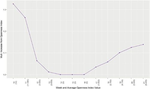
Figures 2 provides a graphical depiction of the estimated relationship of the openness index and weekly robbery rates (results are similar for larceny as the point estimates have similar magnitudes). The horizonal-axis measures weeks into 2020. Week 10 is the last week in 2020 in which all of our cities were completely open, and week 21 is the week of George Floyd’s murder. The value in parentheses under each week is the average value of the openness index across the 23 cities in the openness index analyses in that calendar week. The vertical axis measures the proportional change in the robberies per week associated with the average value for the openness index for that week. Thus, in week 10 when all cities were completely open and the index was at its maximum value of 14, the model predicts that the robbery rate was 33% higher than it would have been had the index been at its minimum of 0 which also coincides with weeks 14–16. Beginning in week 17, on average cities begin opening up, and accordingly the model predicts 3.4% increased robbery rates relative to weeks 14–16. Note by week 21 some lockdown restrictions remained in many cities, but average openness had risen to 6.4, and the model predicts 14% increased robbery rates relative to weeks 14–16.

Fig. 2 Changes in robbery rates during the lockdown relative to typical seasonal levels due to openness index. Week 10 begins on March 8, 2020, and Week 21 begins on May 24, 2020. The value in parentheses is the average value of the openness index in that week.

While we can only speculate on the reason for the null findings for homicide, auto theft, and burglary, notwithstanding we suggest a few possibilities. One is that the degree and success of local efforts to enforce lockdown requirements may mediate local lockdown policies, and data on compliance is difficult to obtain or validate. A second is a potential lack of statistical power due to the somewhat limited variability of weekly changes in the openness index over time and across cities (see Figures 1 and Figure A.6, supplementary materials for summaries of this variability). Third, those committing homicide, auto theft, and burglary may not be sensitive to modest changes in degree of openness but may respond to larger shifts from open to mostly closed.

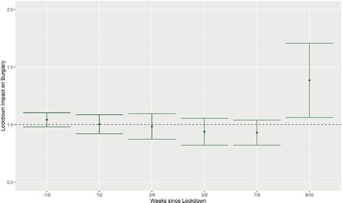
We now turn to the analysis aimed at measuring whether biweekly periods into the lockdown were associated with changing crime rates. As with the openness index analysis above, these analyses also end the week of George Floyd’s murder and largely before associated wide spread protests. Graphs of the results are shown in Figures 1–7. In each of these figures, the black, dashed, horizontal line at one represents the expected crime rate based on the rates in 2020 prior to lockdowns being put in place. The solid green dots indicate the average multiplicative change in crime rates in each of these biweekly time periods relative to seasonal trends in the prior two years and the rates in 2020 prior to lockdowns being instated. The vertical lines are 95% confidence intervals for the biweekly effect estimates. Here we find evidence of significant reductions for all or all but one biweekly period into the lockdown for robbery and larceny as shown in Figures 3 and 4, respectively. Larceny rates appear to fall more quickly at the start of lockdowns whereas robbery rates take about a month to reach their minimum. For homicide, as seen in Figures 5, the pattern is more complex. When each city starts its lockdown, homicide rates are about 20% lower than usual seasonal levels ($p\mathrm{<}0.05$), and there is suggestive evidence based on the point estimates that this decrease persists for another two weeks, but then homicide counts appear to briefly rebound. For the next four weeks, homicide rates appear to be near usual seasonal levels according to the point estimates, and then in the 9th and 10th weeks after each city initiated their lockdown, homicide rates are about 15% higher than usual seasonal levels but with wide confidence intervals. For auto theft (Figures 6) and burglary (Figures 7) all biweekly period estimates are both not significant and fairly similar to usual seasonal levels except for the final week 9–10 period estimates which show abrupt increases for both crime types and are significant (p < 0.05 and p < 0.01, respectively).

Fig. 3 Biweekly 2020 differences in robbery rates during the lockdown relative to typical seasonal levels with 95% confidence intervals.

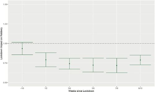
Fig. 4 Biweekly 2020 differences in larceny rates during the lockdown relative to typical seasonal levels with 95% confidence intervals.

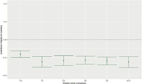
Fig. 5 Biweekly 2020 differences in homicide rates during the lockdown relative to typical seasonal levels with 95% confidence intervals.

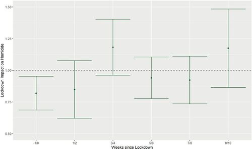
Fig. 6 Biweekly 2020 differences in auto theft rates during the lockdown relative to typical seasonal levels with 95% confidence intervals.

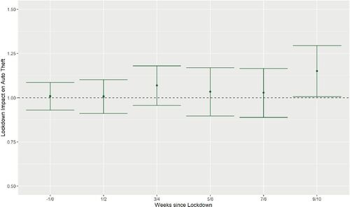
Fig. 7 Biweekly 2020 differences in burglary rates during the lockdown relative to typical seasonal levels with 95% confidence intervals.

Overall, our analyses of crime impacts of lockdown severity and time into the lockdown find strong evidence for larceny and robbery that offense rates dropped during the lockdown and were sensitive to the severity and timing of lockdowns with both crimes rising with increasing openness. We also find more limited evidence that homicide rates were reduced during and immediately before the week in which each city locked down and then fluctuated, while burglary and auto theft rates were at close to typical rates until the very end of the lockdown period when they both abruptly increased in the final biweekly period. These increases may be associated with the early response to George Floyd’s murder as the second week of this period was the week of his murder or to a threshold effect of increases in city openness or other factors. We next turn to an analysis of impacts over the entirety of 2020 where we find more widespread evidence of material impacts.

3.3 Analyses for All of 2020

These analyses are based on Equation (4)(4) $$\begin{array}{c}E\left(y_{\mathit{cwr}}\right)={\lambda }_{\mathit{cwr}}=f(1\ast {\text{Pop}}_c+\alpha +{\gamma }_r+{\theta }_{m\left(w\right)}+{\zeta }_c{}_{}\\ \hspace{1em}+{\beta }_1\ast I_{\left[r=2020\right]}\ast I_{\left[w\le 8\right]}+{\beta }_2\ast I_{\left[r=2020\right]}\ast I_{\left[8<w\le 21\right]}\\ \hspace{1em}+{\beta }_3\ast I_{\left[r=2020\right]}\ast I_{\left[21<w\le 34\right]}\\ \hspace{1em}+{\beta }_4\ast I_{\left[r=2020\right]}\ast I_{\left[34<w\right]}).\end{array}$$(4) which divide 2020 into four periods: Pre-Pandemic, Lockdown, Summer Protests and End of Year and consider how crime rates varied in 2020 in each period relative to usual seasonal patterns. These analyses find evidence of large and significant changes in 2020 compared to companion periods in 2018 and 2019, but the signs of those changes vary by crime type.

Figures 8 summarizes the analysis of homicide. The black, dashed, horizontal line at one represents the expected homicide rate based on seasonal trends in the prior two years. The solid blue dots indicate the average multiplicative change in homicide rates in 2020 relative to seasonal trends in the prior two years. The vertical lines are 95% confidence intervals for the 2020 effect estimates.

Fig. 8 Changes in homicide rates in 2020 compared to typical seasonal trends with 95% confidence intervals.

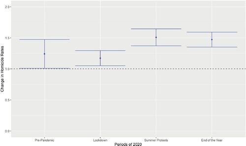
As seen in Figures 8, homicide rates in 2020, relative to prior years, were significantly higher throughout 2020 including during the pre-pandemic period of January and February ($p\mathrm{<}0.05$ for all). The increases are also large. In the pre-pandemic period the increase is nearly 25% relative to 2018 and 2019 homicide rates in January and February. In the final two periods of the year the increase is even larger—about 50% ($p\mathrm{<}0.001$ for both). While this suggests that the already heightened homicide rate in the pre-pandemic and lockdown periods was exacerbated by events post-George Floyd’s murder, the difference between the pre-pandemic point estimate and the two later period point estimates are not statistically significant at the 0.05 level but are significant at the 0.10 level.³ The increase in homicide rates between the lockdown period and the summer protest period, controlling for seasonal trends, is large in magnitude (about 25% higher) and strongly statistically significant ($p\mathrm{<}0.001$).

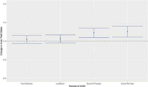
Figures 9 is the counterpart of Figures 8 for auto theft. As seen in Figures 9, in the first two periods of 2020 auto theft rates were similar to those of the prior two years. However, in the summer protest and end of year periods, auto theft rates significantly increased by more than 20% relative to rates over the same months in 2018 and 2019 ($p<0.001$ for both).

Fig. 9 Changes in auto theft rates in 2020 compared to typical seasonal trends with 95% confidence intervals.

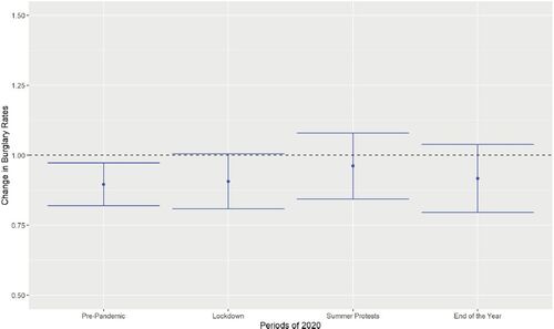
Figures 10 charts the 2020 burglary rate changes. For all four periods the point estimates are negative but only the pre-pandemic estimate is significant at the 0.05 level; the lockdown period estimate is significant at the 0.10 level. These results suggests burglary rates may have been on the a modest 5–10% decline in 2020 but for reasons perhaps unrelated to the pandemic.

Fig. 10 Changes in burglary rates in 2020 compared to typical seasonal trends with 95% confidence intervals.

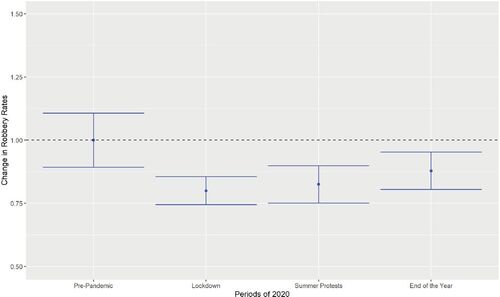
Figures 11 plots robbery rate changes for the four 2020 periods. The pattern is very distinct. In the pre-pandemic period robbery rates were virtually unchanged relative to rates for this two month period in 2018–2019 but declined sharply through all three pandemic periods ($p\mathrm{<}0.01$ for all). The declines were also large—by 14% or more with the largest decrease of 20% occurring during the lockdown period when pedestrian traffic was at its lowest.

Fig. 11 Changes in robbery rates in 2020 compared to typical seasonal trends with 95% confidence intervals.

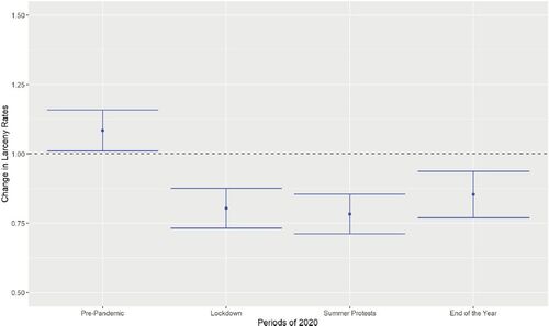
Figures 12 reports results for larceny which are similar to those for robbery. During the three pandemic periods larceny rates declined by 17% or more relative to prior levels in 2018–2019 ($p\mathrm{<}0.01$ for all). This pandemic-related decline is accentuated by the finding that larceny rates in the pre-pandemic period were significantly up relative to 2018–19 levels in January and February ($p\mathrm{<}0.05$).

Fig. 12 Changes in larceny rates in 2020 compared to typical seasonal trends with 95% confidence intervals.

4 Discussion and Conclusions

We find that changes in crime rates during the pandemic from March through December 2020 compared to counterpart periods in 2018 and 2019 were often substantial and were mixed in direction and magnitude. For homicide we find significant increases through all three pandemic periods (lockdown, summer protests, and end of the year) but also for the pre-pandemic period of 2020. We also find significant increases in auto theft during the final half of 2020 spanned by the summer protest period and the end of year period. These increases are also significant compared to the 2020 pre-pandemic period. Balanced against these increases were declines in robbery and larceny throughout the pandemic and some indication of declines in burglary in which all pandemic period point estimates are negative but not statistically significant at the 5% level with the exception of the pre-pandemic period.

Concerning our analyses of the impact of the lockdowns evidence of impacts is more limited. For robbery and larceny, we find evidence that the severity of the lockdown reduced offense rates for these two offense categories but not for homicide, auto theft, or burglary. The analyses of changes in biweekly periods into the lockdown again found evidence of significant declines for larceny and robbery and suggestive results regarding short-term changes for other crime types.

Crime rates by type (e.g., homicide and robbery) usually move in tandem but this did not occur in the pandemic period studied. We instead found a sustained increase in homicide throughout the pandemic and in auto thefts beginning in June and sustained declines in larceny and robbery throughout the pandemic periods. None of the pandemic period estimates for burglary were significant at the 0.05 level but all are negative. In this regard, our findings overall are a challenge for future research to unravel.

As we noted in the introduction our aim was to document changes in crime rates during the pandemic and initial lockdown period but not to ascertain their cause. Regarding the causes of the patterns revealed by our analysis, we can only speculate. One admittedly post hoc and only partial explanation for this unusual pattern relates to opportunity. The decline in robbery rates may have been caused by reductions in numbers of people on streets, particularly at night, thereby reducing robbery targets. Larceny rates may have declined due to closure or reduced foot traffic and possibly increased security (for mask enforcement) in brick-and-mortar retail outlets. The increase in auto thefts may have resulted from the combination of more vehicles sitting idle on the streets and fewer people outside, including police, making it easier to surreptitiously steal the vehicles. Opportunity, however, does not easily explain the findings for homicide and burglary. More time sheltering at home coupled with increased drug and alcohol intake might have given rise to more conflicts that end in a domestic homicide, but press reports on the homicide increase do not attribute it to increases in domestic homicides. Concerning nondomestic homicides, reduced traffic in places such as bars and reductions in young men loitering on the streets due to pandemic restrictions should lead to reductions, not increases, in the types of conflicts that give rise to homicides. As for burglary, more time sheltering at home would reduce opportunities for domestic burglaries, consistent with the trend in the data here. On the other hand, closed businesses might increase opportunities for nonresidential burglaries. Perhaps for burglary, these opposing forces balanced out to no systematic detectable change, but that reasoning may be a stretch.

At the time of this writing in the Spring of 2022, cities across the USA continue to experience the upturn in homicides that we document throughout 2020 including the pre-pandemic period. Local policymakers, namely mayors and police chiefs, must of course respond to this upturn. Understanding location-specific trends is important in determining policy measures going forward. However, recent upticks in the public’s distrust in the police as well as efforts to reimagine local policing in the United States complicate matters for them. These trends have raised questions regarding whether even crime increases as serious as the increase documented here in homicides should necessarily be responded to with increased policing measures or whether alternative strategies should be employed. Furthermore, decreases in larceny and robbery rates that were observed during the pandemic lockdown continued throughout 2020, which means crime rates did not respond uniformly to the pandemic’s onset. Our bottom line on policy recommendations, thus, is that in the absence of a clear understanding of how the pandemic affected crime and in the spirit of evidence-based crime policy, we caution against offering national policy recommendations at this time based on lessons learned from the pandemic “natural experiment.” To do so would erode our standing as scientists offering recommendations based on credible evidence.

Nonetheless, the pandemic natural experiment does provide a unique opportunity for testing various theories of the causes of crime, particularly those related to opportunity which include police presence and contemporaneous social and economic stressors (e.g., poverty, substance abuse, and depression). We recommend that future research examine crime changes during the pandemic based on more detailed crime data complemented by empirical data on policing and economic factors. Our study like all others done to date has been based on analyses of cities for which data was available as the pandemic was unfolding. In all studies conducted thus far, the cities included were far from a complete census of all U.S. cities or a random sample of all cities. Further, to our knowledge there have been no studies of impacts outside of cities in suburban and rural areas or in later stages of the pandemic in 2021. Such studies should be a priority.

Supplementary Materials

Appendix: This supplement consists of full detail regarding the data, variable specifications, and model results as indicated in the text and footnotes. (online_supplement.pdf).

Data Availability Statement

The datasets generated during and/or analyzed during the current study are available in the covid-crime repository, https://github.com/mmeyer717/covid-crime.

Disclosure Statement

The authors report there are no competing interests to declare.

Additional information

Funding

This work was supported by the National Science Foundation (NSF) under RAPID grant agreement no. 2029890. Mikaela Meyer was supported by the National Science Foundation Graduate Research Fellowship Program under Grant No. DGE1745016.

Notes

1 We also tested negative binomial functional form and linear regression with the log of the weekly crime rate specification for higher rate crimes. In all cases, results were similar. Results for the outcome and functional form specification sensitivity analyses are available upon request.

2 These results are available upon request.

3 We also note that analyses of aggravated assaults, which are often events very similar to homicide but where the victim’s injuries are not fatal, only partially mirror our findings for homicide. While aggravated assault rates were significantly up in the summer protest and end of year periods (p <0.01), the point estimates for the first two periods fall well short of statistical significance and are close to zero. These results are reported in Table B.3 in the supplementary materials. Recall that we decided against showcasing results for aggravated assaults due to concerns about the completeness of the aggravated assault data.

References

- Abrams, D. (2020), “COVID and Crime: An Early Empirical Look (SSRN Scholarly Paper ID 3674032)” Social Science Research Network. DOI: 10.2139/ssrn.3674032.
- Ashby, M. P. J. (2020), “Initial Evidence on the Relationship Between the Coronavirus Pandemic and Crime in the United States,” Crime Science, 9, 6–21. DOI: 10.1186/s40163-020-00117-6.
- Asher, J., and Horwitz, B. (2020), “It’s Been ‘Such a Weird Year.’ That’s Also Reflected in Crime Statistics.” The New York Times. Available at https://www.nytimes.com/2020/07/06/upshot/murders-rising-crime-coronavirus.html.
- Becker, D., and Corley, C. (2020), “Violent Crime Increases In Several Cities Nationwide.” NPR. https://www.npr.org/2020/08/14/902456117/violent-crime-increases-in-several-cities-nationwide.
- Campbell, J. (2020). “Violent Crime Soars during Pandemic as Confidence in Police Takes a Hit.” CNN. Available at https://www.cnn.com/2020/08/16/us/violent-crime-soars-confidence-in-police-takes-hit/index.html.
- Campedelli, G. M., Aziani, A., and Favarin, S. (2021), “Exploring the Effect of 2019-nCoV Containment Policies on Crime: The Case of Los Angeles,” American Journal of Criminal Justice, 46, 704–727. DOI: 10.31219/osf.io/gcpq8.
- CNN. (2020), “This is where each state is during its phased reopening.” CNN. Available at https://www.cnn.com/interactive/2020/us/states-reopen-coronavirus-trnd//.
- Coote, D. (2020), FBI: Murders Climbed Amid a Decrease in Violent Crime in 2020.” UPI. Available at https://www.upi.com/Top_News/US/2020/09/15/FBI-Murders-climbed-amid-a-decrease-in-violent-crime-in-2020/9471600225926/.
- FBI (2020), “Overview of Preliminary Uniform Crime Report, January–June, 2020” [Press Release]. Available at https://www.fbi.gov/news/pressrel/press-releases/overview-of-preliminary-uniform-crime-report-january-june-2020.
- Graham, D. A. (2021), “Murders Are Spiking in America.” The Atlantic. Available at https://www.theatlantic.com/ideas/archive/2021/09/2020-homicide-spike-was-real/620183/.
- Hilsenrath, J. (2020). “Homicide Spike Hits Most Large U.S. Cities.” Wall Street Journal. Available at https://www.wsj.com/articles/homicide-spike-cities-chicago-newyork-detroit-us-crime-police-lockdown-coronavirus-protests-11596395181.
- Lopez, G. (2020). “The Rise in Murders in the US, Explained.” Vox. Available at https://www.vox.com/2020/8/3/21334149/murders-crime-shootings-protests-riots-trump-biden.
- McCarthy, N. (2020), “Major American Cities See Sharp Spike in Murders In 2020 [Infographic].” Forbes. Available at https://www.forbes.com/sites/niallmccarthy/2020/08/04/major-american-cities-see-sharp-spike-in-murders-in-2020-infographic/.
- Mohler, G., Bertozzi, A. L., Carter, J., Short, M. B., Sledge, D., Tita, G. E., Uchida, C. D., and Brantingham, P. J. (2020), “Impact of Social Distancing during COVID-19 Pandemic on Crime in Los Angeles and Indianapolis,” Journal of Criminal Justice, 68, 101692. DOI: 10.1016/j.jcrimjus.2020.101692.
- Piquero, A. R., Riddell, J. R., Bishopp, S. A., Narvey, C., Reid, J. A., and Piquero, N. L. (2020), “Staying Home, Staying Safe? A Short-Term Analysis of COVID-19 on Dallas Domestic Violence,” American Journal of Criminal Justice, 45, 601–635. DOI: 10.1007/s12103-020-09531-7.
- Rosenfeld, R., Abt, T., and Lopez, E. (2021), “Pandemic, Social Unrest, and Crime in U.S. Cities: 2020 Year-End Update.” National Commission on COVID-19 and Criminal Justice. Available at https://covid19.counciloncj.org/2021/01/31/impact-report-covid-19-and-crime-3/.
- Struett, D. (2020). “Chicago Nears 700 Homicides in 2020, a Milestone Reached Just One Other Time Since 1998.” Chicago Sun-Times. Available at https://chicago.suntimes.com/crime/2020/11/18/21573378/chicago-homicides-700-murders-2020-gun-violence-shootings.
- The New York Times (2020), “See Coronavirus Restrictions and Mask Mandates for All 50 States.” The New York Times. Available at https://www.nytimes.com/interactive/2020/us/states-reopen-map-coronavirus.html.
- U.S. Census Bureau (2020), “City and Town Population Totals: 2010-2019: Subcounty Resident Population Estimates: April 1, 2010 to July 1, 2019 (SUB-EST2019).” The United States Census Bureau. Available at https://www.census.gov/data/datasets/time-series/demo/popest/2010s-total-cities-and-towns.html.
- WorldPopulationReview.com (2020), “The 200 Largest Cities in the United States by Population 2020.” Available at https://worldpopulationreview.com/us-cities.