Financial Literacy and Perceived Economic Outcomes

Abstract

We explore the relationship between financial literacy and self-reported, reflective economic outcomes from respondents using survey data from the United States. Our dataset includes a large number of covariates from the National Financial Capability Study (NFCS), widely used by literacy researchers, and we use a new econometric technique developed by Hahn et al., designed specifically for causal inference from observational data, to test whether changes in financial literacy infer meaningful changes in self-perceived economic outcomes. We find a negative treatment parameter on financial literacy consistent with the recent work of Netemeyer et al. and contrary to the presumption in many empirical studies that associate standard financial outcome measures with financial literacy. We conclude with a discussion of heterogeneity of the financial literacy treatment effect on household income, gender, and education level sub-populations. Our findings on the relationship between financial literacy and reflective economic outcomes also raise questions about its importance to an individual’s financial well-being.

KEYWORDS:

• Causal inference
• Financial literacy
• Financial well-being
• Perceived economic outcomes
• Regularization

1 Introduction

Is financial literacy associated with a household achieving a higher perceived economic outcome? There is a natural presumption that basic literacy is good and gradations of increasing financial literacy are better. Interest and education in financial literacy in the United States have become widespread and institutionalized by the Federal Reserve System and the Consumer Finance Protection Bureau.¹ Books on personal finance, investing, and wealth creation have become as ubiquitous as books on health and weight loss.

A presumption underlying an investment in financial knowledge is that a household will have a better chance at optimizing their living standard if they are financially adept. Specialized knowledge may be important since just being well-educated does not enable competence about personal finance. Mitchell and Lusardi (2015) found that increased education and financial literacy are positively correlated, yet they find less than 50% of college-educated students can successfully answer three key financial literacy questions, and less than 64% of students with a post-graduate education can answer all three questions correctly. Perhaps “interventionist” activity is needed. Campbell (2016) argued that important questions about financial regulations surrounding household finance are ripe for the attention of economists because there is not much known about how consumer financial regulatory costs would be offset by its benefits.

The intent of financial literacy training and policy prescriptions is to lead to better financial decisions. But what is a good decision? The motivation or judgment about a financial activity can be difficult to assess by researchers working with survey data in which respondents are being asked about their financial makeup. When working with such data, assumptions have to be made, and there is heterogeneity in assessing a respondent’s personal economic outcome, precisely because it is an individual measure. Is it really a bad choice to have a car loan, student loan debt, or spending that exceeds income in the current month? It may not be. Economic theory is clear that household borrowing is just as reasonable as saving.² Netemeyer et al. (2018) assert that care must be taken to not “confound” particular financial behaviors with financial well-being.³ To best understand the effects of policy prescriptions targeted toward increasing financial knowledge, we construct an outcome for financial well-being. In this article, we use a composite index of an individual’s economic satisfaction to measure whether an individual’s financial literacy raises their perception of their economic standing.

The conceptual question we investigate is in contrast to the large body of research summarized by Hastings, Madrian, and Skimmyhorn (2013) and Lusardi and Mitchell (2014) that studies key questions around financial literacy and its relation to education choices, the timing of education delivery during an individual’s life cycle, public policy prescriptions, and regulatory intervention. In much of the financial literacy literature, questions are posed and hypotheses are tested with formulations that associate financial literacy with standard financial outcome measures, for example, the number of times an individual makes a financial mistake or the use of a payday loan. Regardless of the outcome under investigation, it is still not well understood whether financial literacy is causally related after conditioning on many relevant covariates. Hastings, Madrian, and Skimmyhorn (2013) expressed the importance of causal assessments between literacy and economic outcomes to financial education policy-making. To paraphrase, “is it financial literacy that leads to better economic outcomes, do certain economic behaviors lead to more financial literacy, or do factors such as general intelligence and an interest in financial matters contribute to both higher levels of financial literacy and better financial outcomes?”⁴

Over the past 20 years, social scientists have been exploring “financial well-being” and how this attitudinal construct fits within an individual’s determination of their overall well-being. Netemeyer et al. (2018) review this literature which, in the spirit of predicting an outcome related to household finance, is parallel to this article. For financial literacy researchers of any proclivity, the authors offer a new and important way to define financial well-being and find it to be a significant predictor of overall well-being.⁵

In this article, we apply a methodology that strengthens our understanding of the causal connection between financial literacy and financial outcomes, perceived or not, through a treatment effect estimation procedure applied to publicly available data widely used by literacy researchers.⁶ We begin by isolating economic outcomes from behaviors using the data generated from FINRA’s complete 2015 and 2018 National Financial Capability Survey studies. We identify three survey questions that reveal actual respondent self-perceived economic outcomes. Further, we categorize a number of good and bad financial practice behaviors and include numerous other respondent and household factors that are plausibly related to economic outcomes, including a financial literacy treatment variable. In this study, we are interested in a primary question:

Is there a causal relationship between the level of an individual’s financial literacy and their perception of their current economic condition?

There are two important aspects of this question to address. First, we focus on a reflective household financial measure that is a proxy for the accumulation of a household’s past financial decisions, current financial resources, and future prospects (expected human capital, an inheritance, bequest planning and so forth). This is in contrast to many financial literacy studies that attempt to look at a specific financial activity that when viewed in isolation is likely to be conflated by other decisions within the household economy.

Second, there is significant confounding in the survey data since financial literacy is correlated with both a dependent variable measuring economic outcome and characteristics measured for each person in the survey. Also, the dimensions of any final sample from the NFCS study are characterized by a large number of covariates and a relatively limited number of observations making more traditional estimation approaches problematic.⁷ To mitigate the effects of these statistical issues, we apply the work of Hahn et al. (2018) who call on recent research in treatment effect estimation and machine learning. We employ the authors’ data-driven approach to mitigate treatment effect estimation bias.⁸

After a review of the literature, the study proceeds by defining a new variable from information in the NFCS dataset: a household’s perceived economic outcome. We use answers to three questions to construct an economic outcome index using principal component analysis, and we then estimate a model relating economic outcome to financial literacy and a large set of covariates using a regularized regression methodology.

Following a brief discussion of the control variables, we provide background on the estimation approach and report a treatment effect estimate that strongly supports a negative relationship between financial literacy and economic outcome. Our findings are based on the NFCS 2015 and 2018 surveys and control for all available covariates that potentially account for variation in our treatment and outcome variables.⁹ The estimation approach used in this article permits controlling for all covariates, instead of more traditional empirical analyses where plausible (small) subsets of covariates are selected by the researcher and coefficient estimates are compared across model specifications. We advocate for an approach where all covariates are used (Hahn et al. 2018; Hahn, Murray, and Carvalho 2020) since it mitigates treatment effect bias due to confounding. The contrast between the approach used here and traditional approaches that fit several “smaller” models based on sets of covariates is worth emphasizing. Hand-selecting small sets of covariates is implicitly biasing the treatment effect estimate and our approach avoids this empirical mistake. We conclude by introducing future work on understanding treatment effect heterogeneity. These results suggest that the effect of literacy on an individual’s appraisal of their economic condition becomes increasingly negative as household income increases.

1.1 Literature Review

It is well-documented that U.S. citizens have low levels of financial knowledge and make financial “mistakes.” Calvet, Campbell, and Sodini (2009) created an index of financial sophistication from mistakes related to under diversification, risky share turnover and the disposition effect and find that less sophistication is related to individuals with less wealth, smaller family size, less education and less financial experience.¹⁰ Choi, Laibson, and Madrian (2011) found that more than a third of employees do not take advantage of an employer match to a 401(k) plan when it is clearly to their benefit to do so.¹¹ Keys, Pope, and Pope (2016) found that 20% of households do not refinance their mortgage even when it is to their benefit, and Agarwal, Ben-David, and Yao (2017) found the individuals who opt for points in their mortgages, a poor financial choice in their analysis, are less responsive to interest rate changes and preferred refinancing behavior.

To expand financial literacy, many states have implemented education reforms at the K-12 level. The intensity of state-mandated personal finance education varies by states and in 2020 twenty-four states require a personal finance course to be offered.¹² There is a growing body of research on the relationship between state-mandated financial education and financial behavior using a variety of datasets. Brown et al. (2016) found a significant causal relationship between more financial education and better non-student debt repayment behavior among adults ages 19–29 using the Council on Economic Education’s “Survey of the States.”¹³ Using NFCS data from 2012 and 2015 among respondents from 19 through 31, Harvey (2019) found financial education reduced the reliance on payday loans, but not other “alternative” financial services among survey respondents. Urban et al. (2018) explored financial education and credit scores among a sample of 18 through 21 year-olds using Georgia and Texas as financial education regimes and contrasting each regime with a synthetic control state using data from the Consumer Credit Panel (CCP). The researchers found that financial education improved credit repayment behavior and credit scores, and that the amplification of the results were higher in Georgia where the mandated financial education requirement goes deeper in teacher training and student testing. Stoddard and Urban (2020) examined whether high school financial education influenced borrowing behavior of incoming freshmen at 4-year colleges using financial aid data from the National Postsecondary Aid Study (NPSAS) from 1999 through 2011. The time frame of the sample permitted the authors to compare college students from the same states before and after mandated financial education. The authors’ found that while borrowing for college is slightly higher among those students with a financial education background, loan choices were toward lower cost subsidized loans rather than higher cost private loans, and credit card usage was lower.

A contrasting contribution to the financial literacy literature suggests public investments in financial education may not be helpful in solving the problem of poor financial choices because consumers will never be able to keep up with the complexity of financial products. Willis (2008) confronted the idea that financial education is inherently a good idea by taking the view that a “financial regulation-through-education policy model” imposes costs on those aspiring to be financial literate that are significantly higher than the benefits from the financial literacy gained.¹⁴ Policymakers who promote financial literacy as important intend, at least partly, to have the individual bear responsibility for the management of his or her financial future. Indeed, Willis (2011) asserted that financial regulation replaced by financial education is a “fundamental fallacy.”¹⁵ The individual would always be chasing the details of new product innovation and once the consumer shortens their information disadvantage, Willis argues that the industry would “outmaneuver” them.¹⁶

Lusardi, Michaud, and Mitchell (2017) built a dynamic life-cycle model in which financial knowledge acquisition is considered an endogenous process over the lifetime of an individual. The value in learning how and where to invest savings depends on many factors including longevity, demographic differences and post-retirement income replacement rates provided by social security retirement benefits. The researchers have financial knowledge manifest itself through either a basic savings vehicle such as a checking account or a more sophisticated investment technology in which a higher risky return is available albeit at a higher knowledge acquisition cost. The researchers measured an economic outcome as the median wealth to income ratio at retirement and found that differences in economic outcomes at retirement are more impacted by financial knowledge than other factors such as mortality, demographics, social security retirement benefits. An additional implication of this work is while less costly financial knowledge acquisition would be welfare enhancing, life-cycle expected utility maximizers who have less to gain from financial education programs “can boost saving in the short run, but it might have little enduring impact in terms of boosting lifetime wealth.¹⁷”

Another path toward financial literacy is to rely—at least partially—on the literacy of others, for example, advisors. Calcagno and Monticone (2015) started with a premise that those who are less financially literate may benefit from more personal finance advice or derive more value from a financial adviser. They construct a theoretical model that considers an adviser who has the ability to sell investments and is compensated by a proportional commission linked to the size of the investment. The adviser’s customer may be asymmetrically informed about the attributes of prospective investments. Considering incentives, penalties, and information costs, their model predicts that those who are better informed are more likely to invest in risky assets and use a financial adviser. Indeed, the authors use bank survey data from Italy to find empirically that utilization of financial advisers is higher among those who are already financially literate, and that financial literacy is positively related to the probability of investing in risky assets; results consistent with the implications from Lusardi, Michaud, and Mitchell (2017).¹⁸ In a different yet relevant study, Balasubramnian and Brisker (2016) used 2012 NFCS survey data and an instrumental variables approach to mostly corroborate Calcagno and Monticone’s empirical results. Balasubramnian and Brisker defined advisers by their role with a survey participant (e.g., Investment adviser, Debt Counselor, Tax adviser and so forth) if such a relationship existed at all.¹⁹ The researchers found a positive relationship between working with an investment financial adviser and financial literacy, although they found a negative relationship for those who worked with a debt consolidation adviser.

The literature to date supports the conclusions that households err in their financial decision-making, more highly educated individuals are not inclined to be better at making financial decisions, and that investments in financial education can lead to changes in certain financial behaviors. More sophisticated individuals may be more inclined to hire financial advisers, but is that a good idea, and do individuals of any sophistication level know there are differences in how advisers are paid and the incentives that drive their recommendations? There are good reasons for consideration of a third-party who can force guidance on consumers in the spirit of the arguments presented by Campbell (2016). The existing literature suggests that not enough is known about whether higher levels of financial literacy can create a good economic outcomes or at least the perception of one. Indeed, Netemeyer et al. (2018) found a negative correlation between financial literacy and expected future financial security using data from the Survey Sampling International online panel. Of potential importance to Netemeyer et al. (2018)’s result is their untangling objective financial literacy from “correlates of financial knowledge,” posited to be important to explaining financial well-being. Consequently, Netemeyer et al. (2018) explored “a willingness to take investment risks,” a “willingness to plan,” and “financial self-efficacy,” as well as financial literacy and found financial literacy was negatively related to a self-assessed measure of future financial security while the other attributes were positively related. One implication from their research is that objective financial literacy at a given point in time may not be as important as a taste for risk, organization, and knowing how to find answers to financial questions. An additional implication relevant to this study is that more highly financially literate individuals are inclined to feel worse off about their economic futures.

While our primary interest is to offer evidence on whether financial literacy has a causal effect on the perceived economic outcomes of households, we have a secondary interest related to financial behaviors. That is, we want to know whether financial behaviors commonly thought of as “good” or “bad” have the expected relationship with economic outcome. Evidence that literacy, behavior, or both are important to household economics would have implications for education and policy choices and the allocation of resources to these activities.

2 The Study

What is an Economic Outcome? The NFCS survey provides reasonable proxies of a respondent’s assessment of their economic outcome based on answers to survey questions placed throughout the questionnaire.²⁰ We identified three questions used in both the 2015 and 2018 National Financial Capability Studies that are representations by respondents about their current financial circumstance.²¹ They are the following:

1. “Overall, thinking of your assets, debts and savings, how satisfied are you with your current personal financial condition?”

2. “In a typical month, how difficult is it for you to cover your expenses and pay all your bills?”

3. “How strongly do you agree or disagree with the following statement?—I have too much debt right now”

Defining an economic outcome from survey data that does not contain financial metrics can, at first glance, pose a challenge. However, the NFCS survey questions listed above are asking respondents to reflect on their economic comfort which shifts the judgment about how an economic outcome might be defined by a researcher toward the judgment of the respondent. Answers to the three survey questions are ordinal, and we use a principal component analysis to aggregate answers to multiple questions with ordinal outcomes to create a single economic outcome measure.

The Data and Analysis. We start with the combined full dataset from the 2015 and 2018 NFCS studies made available to us by FINRA.²² As is common in survey data, many observations contain variables with answers coded as missing. In addition to missing values, answers to certain questions contain the responses, “Don’t know” or “Prefer not to say.” In our dataset 38 of the 114 aggregate variables are missing responses. Analogous to other standard modeling approaches, we omit observations with these features as do all authors who use the NFCS datasets (see, e.g., Lusardi, Mitchell, and Oggero 2020). Importantly, in our empirical approach we are not restricting the covariate space. In this manner, correct inferences can be made and generalizations can follow from the structure of the sample. Most importantly, this permits us to use as much covariate information as possible.²³ The largest set of complete data for which we are able to include a sufficiently rich subset of survey variables includes 4694 observations and 33 continuous and categorical variables.²⁴ These covariates are described in Table 4. After expanding out the categorical variables into their binary representation, our set of covariates numbers 532. Note that in the Appendix, we compare our sample with the original NFCS 2015 and 2018 survey along the chosen covariates which highlights the compatibility of our sample and provides guidance, based on covariate distributions, about the types of individuals to which applies our inference of literacy on economic outcome.

Table 4 This table presents the additional control variables that we consider in our empirical analysis.

NFCS	Panel A Description: Good practice financial behaviors
J5	Do you have emergency funds that can cover 3 months of expenses?
J6	Are you saving for your children’s college education?
F2_1	Over the past 12 months have you always paid your credit card in full?
C5	Do you or your spouse regularly contribute to a thrift plan, 401(k) or IRA
	Panel B Description: Bad practice financial behaviors
B4	Do you overdraw from your checking on occasion?
E15	How many times have you been late with your mortgage payment?
E20	Do you owe more on your home than it is worth?
F2_2	Over the past 12 months have you carried a balance and were charged interest?
F2_3	Over the past 12 months, in some months I paid the minimum payment only
F2_4	Over the past 12 months, I incurred credit card late fee
F2_5	Over the past 12 months, I was charged an over the limit fee for exceeding my credit line
F2_6	Over the past 12 months, I used my card for a cash advance
G25_1	In the past 5 years, how many times have you taken out an auto title loan?
G25_2	In the past 5 years, how many times have you taken out a payday loan?
G25_4	In the past 5 years, how many times have you used a pawn shop?
G25_5	In the past 5 years, how many times have you used a rent-to-own store?
	Panel C Description: Other controls
A3	Gender of respondent
log(A3A)	The log of the age of the respondent
A4A	Ethnicity subcategory
A5_2015	Highest level of education
A7	Living arrangement in the household
A7A	Marital status that includes a living with partner choice
A8	Household’s income
A9	Best describes your current employment or work status
A10	Best describes your spouse/partner work status
A11	Children who are financially dependent
AM21	Armed forces member?
G1	Do you have an auto loan?
G20	Do you have any unpaid medical bills?
J2	When thinking of your financial investments, how willing are you to take risks?
J3	Would you say your spending was less than, more than, or about equal to your income?
STATEQ	The state of the respondent
Time	Indicates whether the dataset is 2015 or 2018

NOTE: They are categorized as (i) good practice financial behaviors, (ii) bad practice financial behaviors, and (iii) other controls.

Dependent Variable. Our dependent variable of interest is an economic outcome index that is created from the responses to the economic outcome questions which are summarized in Table 1. Questions 1, 2, and 3 are measured on integer scales from 1 to 10, 1 to 3, and 1 to 7, respectively. The mean, minimum, and maximum values are displayed in Table 1.

Table 1 (left) Responses to questions used to construct the economic outcome (dependent) variable: Summary statistics for quantitative variables across the NFCS sample of 4694 observations. (right).

	Q1	Q2	Q3
mean	6.61	2.51	4.21
min	1	1	1
max	10	3	7
SD	2.35	0.64	2.17

NOTE: Responses to questions used to construct the economic outcome (dependent) variable: Summary statistics for binary variables across the NFCS sample of 4694 observations.

These three questions comprise our measure of a perceived economic outcomes for individuals in the sample. In Section 3, we discuss how we combine this information from multiple outcomes into a single, meaningful measure.

Financial Literacy Variable. The connection between economic outcomes and financial literacy is tested with a measure for financial literacy that is the total number of correct answers to six financial literacy questions included in the 2015 survey and reported in Table 2.²⁵ The third column of Table 2 summarizes the percentage of correct answers for each of the six financial literacy questions across the sample. Relatively higher proportions of respondents were successful at answering correctly the savings account growth question (“Interest rate”) and the mortgage payment and mortgage interest paid (“Mortgage”) question. More than 60% of respondents did not understand the relationship between a bond’s value and market interest rates (“Bond price”), and about half of the respondents proved adept at questions related to inflation, the rule of 72 and risk. The six questions taken together across the final sample showed a mean number of correct answers equal to 3.86.

Table 2 Financial literacy assessment questions considered from the FINRA dataset.

Concept addressed	Question	% Correct
Interest rate	Suppose you had $100 in a savings account and the interest rate was 2% per year. After 5 years, how much do you think you would have in the account if you left the money to grow?	86%
Inflation	Imagine that the interest rate on your savings account was 1% per year and inflation was 2% per year. After 1 year, how much would you be able to buy with the money in this account?	68%
Bond price	If interest rates rise, what will typically happen to bond prices?	35%
Rule of 72	Suppose you owe $1000 on a loan and the interest rate you are charged is 20% per year compounded annually. If you didn’t pay anything off, at this interest rate, how many years would it take for the amount you owe to double	43%
Mortgage	15-year mortgage typically requires higher monthly payments than a 30-year mortgage, but the total interest paid over the life of the loan will be less. Measurement Level: Nominal	92%
Risk	Buying a single company’s stock usually provides a safer return than a stock mutual fund.	62%

NOTE: Displayed are the financial concept addressed, question asked, and the percentage who answered correctly within our sample.

Table 3 reports three additional views of the sample’s financial literacy disaggregated by three age groupings and level of highest educational achievement. In Panel A of Table 3, actual financial literacy, measured by the mean number of correct answers to the set of financial literacy questions, is higher among those with at least some college education and older age groups. These groups also exercise higher levels of financial investing as can be seen in Panel B in which the mean values of respondent answers to the question “not including retirement accounts, do you have any investments in stocks, bonds, mutual funds, or other securities,” are reported.²⁶ Self-assessment of financial knowledge reported in Panel C does not necessarily run parallel to tested financial literacy. Respondents were asked: “On a scale from 1 to 7, where 1 means very low and 7 means very high, how would you assess your overall financial knowledge?” Contrary to actual financial knowledge, self-assessment of financial knowledge is less informative: mean values tend to run toward the more knowledgeable end of the scale across all education and age groupings.

Table 3 Financial literacy, financial investing, and self-assessment of overall financial knowledge by educational attainment level and age category.

Panel A	Financial literacy
Education Level	<45	45–60	>60
No high school	2.50	3.33	3.00
High school	2.84	3.55	3.87
GED	2.81	3.54	3.67
Some college	3.43	4.00	4.02
Associate degree	3.36	3.96	4.25
Bachelor degree	3.83	4.42	4.61
Post graduate degree	3.90	4.71	4.77
Panel B	Financial investing
Education Level	<45	45–60	>60
no high school	1.62	1.67	2.00
high school	1.49	1.59	1.40
GED	1.42	1.65	1.67
some college	1.50	1.57	1.51
associate degree	1.51	1.53	1.31
bachelor degree	1.42	1.38	1.36
post graduate degree	1.38	1.28	1.27
Panel C	Self-assessment of financial knowledge
Education Level	<45	45–60	>60
No high school	6.00	5.33	6.00
High school	5.58	5.38	5.40
GED	5.83	5.67	5.33
Some college	5.60	5.42	5.69
Associate degree	5.49	5.44	5.56
Bachelor degree	5.62	5.67	5.86
Post graduate degree	5.76	5.72	5.59

Additional Control Variables. Generally, descriptive statistics of the NFCS data have been reported by many researchers including the NFCS itself, and we follow accordingly for the data used in this article.²⁷ For discussion, we segregate the controls into socio-economic factors and financial behaviors. The socio-economic factors are numerous and include information about the respondent’s age, education, and marital status along with the other variables listed in Table 4.

We present the listing of variables associated with the survey questions and answers that are indicative of financial behaviors that we categorize as good practice (Panel A) and bad practice (Panel B). In Panel A we included the set of variables based on questions a positive answer to which would more clearly indicate that the respondent is more active in thinking about financial planning. Having emergency funds, a budget, long-term financial goals, an implemented savings plans and the pay down of a credit card bill are indicative of both planning and financial practice. By contrast, in Panel B of Table 4 a longer list of variables, positive answers to which are more indicative of financial stress. Many of these variables indicate higher debt loads, or consumption greater than current resources.

3 Empirical Analysis

3.1 Economic Index Construction

We construct a single economic outcome index for each observation combining the answers to the three questions summarized in Table 1 using a common dimension reduction technique. These three variables provide self-reported proxies for the economic health. Answers to these questions are certainly correlated.²⁸ Since there is overlapping information present in each variable, our first methodological step is to extract the relevant variation among the original three variables, and we use principal component analysis (PCA) to accomplish this dimension reduction task. Specifically, we construct our economic index by projecting the three original variables onto the first eigenvector. This provides a univariate variable which uses information from the three questions along the highest variance dimension of these economic outcome proxies.

Figure 1 displays boxplots corresponding to the economic health variables and the constructed economic outcome index. The economic outcome index is shown on each vertical axis and is scaled to have zero mean and unit variance. Positive values of the index correspond to favorable economic outcomes, and negative values correspond to unfavorable outcomes. Question 1 (Q1) deals with how satisfied the respondent is with their financial condition. Low levels of satisfaction given by answer on the far left of the x-axis are associated with (on average) negative values for the index. As satisfaction increases, the conditional expectation of the index (given by the black lines in the center of the boxplots) increases.

Fig. 1 Values of the economic outcome index separated by answers to original financial outcome questions. Each subplot corresponds to a single question, and the individual boxplots display the distribution of the economic outcome index for the set of respondents that answered accordingly.

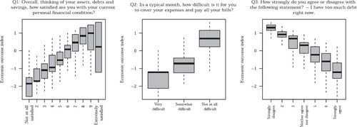
Q2 displays conditional distributions of the constructed economic outcome index related to the difficulty in covering monthly expenses and paying off bills on a three level scale. There are separations in the conditional distributions where the “Very difficult” respondents possess negative index values, while the “Not at all difficult” respondents have markedly higher, and on average positive, index values.

The final question measures agreement with the following statement: “I have too much debt right now.” There are seven levels of agreement. As the levels go from “Strongly disagree” to “Strong agree,” we observe a monotonic trend from positive index values to negative index values—especially in expectation. On average, respondents who feel that their personal debt is high are those with negative economic outcomes. Taken together, the conditional distributions displayed in Figure 1 provide evidence that the economic index is measuring what we want: negative index values imply economic instability and financial distress and positive values imply economic stability.

3.2 The Estimation Approach

The establishment of an economic outcome index from the NFCS question set permits us to focus on the question of whether financial literacy has an effect on economic outcome. The problem is framed in terms of the following regression model for observation i:(1) $$Y_i=\alpha Z_i+{\mathrm{X}}_i^t\beta +{\nu }_i,$$(1) where ${\mathrm{X}}_i$ is a vector of control variables, β is a vector of the control effects, Z_i is a continuous scalar treatment variable and α is a scalar regression coefficient. We assume the errors, ν_i, are normally distributed with zero mean and unknown variance. In our application, Z_i is a measure of financial literacy—the number of correct answers to the six questions outlined in Section 2. The dependent variable Y_i is the economic outcome index described in Section 3.1. The control variables (covariates) ${\mathrm{X}}_i$ are the 41 additional characteristics of the observations displayed in Table 4. For ease of interpretation, we scale Z_i and ${\mathrm{X}}_i$ to have zero mean and unit variance. This allows us to estimate Model 1 without an intercept.

α is the parameter of interest. Accurate estimation of α must be done by including the “right” controls, where the formal definition for “right” is(2) $$\text{cov}(Z_i,{\nu }_i|{\mathrm{X}}_i)=0.$$(2)

This condition ensures the desired counterfactual interpretation of α as the amount that economic outcome (Y) would change if literacy (Z) were increased by one unit.

For our analysis, we, like other researchers, quickly encounter the question: Which controls from the NFCS study should we select, and how does that selection impact the estimation of α? Omitted variable biases are generally well known. Traditionally, one selects multiple sets of plausible control variables. “Plausibility” for inclusion in the model may be based on economic theory, anecdotal observation, or past empirical findings, but the lack of rigor in this approach is well known (Leamer 1978, 1983). To resolve these problems and to capture the causal inference, we use the approach outlined in Hahn et al. (2018) in which the large set of potential controls in the NFCS dataset can be informed from statistical regularization. Put simply, this approach allows the analyst to include every measured control variable, instead of hand selecting a subset. The latter will lead to unknown biasing of the causal effect, while the former guarantees that any bias is mitigated.

Regularized Regression for Treatment Effect Estimation. Our desire to use predictive methods for causal inference stems from the need to “predict” an economic outcome in a “counterfactual world.” In our dataset, we have a fixed set of individuals with varying levels of financial literacy and tied to each individual is a measured level of financial literacy. However, we would like to ask the question: How would an individual’s outcome change if her literacy increased? This question exposes the main challenge of causal inference. We are “missing data” since we are unable to observe the counterfactual outcome of an individual with a different literacy level (Imbens and Rubin 2015). We use a two equation variant of Model 1 coupled with a useful reparameterization.²⁹ To do this, we couple Model 1 with a model for financial literacy (Z) conditional upon the covariates:(3) $$\begin{array}{cc}\text{Selection Eq}.:\hfill & Z=\mathrm{X}\gamma +\mathrm{ϵ},\mathrm{ϵ}\sim N(0,{\sigma }_{\mathrm{ϵ}}^2),\hfill \\ \text{Response Eq}.:\hfill & Y=\alpha Z+\mathrm{X}\beta +\nu ,\nu \sim N(0,{\sigma }_{\nu }^2).\hfill \end{array}$$(3)

The first model attempts to predict literacy using observed characteristics of the observations. Importantly, the residual error ${\sigma }_{\mathrm{ϵ}}^2$ will gauge the degree of confounding—how well the characteristics of the observations describe the resulting financial literacy.

Jointly estimating the model for $Z|\mathrm{X}$ and $Y|Z,\mathrm{X}$ can lead to better inferences about α. The intuition follows in two steps. First, learn about which $\mathrm{X}$’s “matter” for Z from the selection equation. Second, use that information to properly “control” for those $\mathrm{X}$’s in the response equation. In both steps, statistical regularization via Bayesian priors is used to determine the meaningful $\mathrm{X}$’s. In our estimation approach, there is no need to select a subset of characteristics in $\mathrm{X}$ to control for in the selection and response equations a priori. Instead, all available covariates are included in our model, and the estimation procedure automatically determines which are relevant.

Several recent papers focus on estimating the causal effect α using state-of-the-art Bayesian modeling (Hahn et al. 2018; Hahn, Murray, and Carvalho 2020). This research discusses how to deploy statistical regularization (through Bayesian shrinkage priors) to allow for the inclusion of all covariates in the selection and response equations in Model 3 and accurately estimate the causal effect. In this article, we employ a two-step approach described in Hahn, Murray, and Carvalho (2020) using Model 3. First, we obtain an prediction of literacy $\widehat{Z}$ from the selection equation. Second, we augment the covariates in the response equation to include this prediction, $\tilde{\mathrm{X}}=[\widehat{Z}\mathrm{X}]$, and estimate the causal effect α.³⁰

3.3 Findings

The regularization approach in this article informs the process of identifying appropriate controls from the total number of controls (p = 532) across the final dataset with 4694 observations. Included in the model is the set of variables in Table 4 plus several interactions terms. The interaction terms include log(Age), gender, and time, each interacted with all other variables displayed in Table 4. We report the top line estimate of the causal effect α in Table 5. Our analysis finds that not only is the effect of financial literacy on economic outcome negative, but also that this effect is strongly significant since the posterior credible interval does not include zero. At first glance, the result is surprising because financial institutions, policymakers, educators and personal finance writers assert that financial literacy is as important as the ability to read and write; competence is required for economic satisfaction. Saving, little debt and an understanding of how to invest are prescriptions for how to be financially independent or financially happy. These views are corroborated by academic studies which hypothesize financial literacy to be related to a certain financial behavior that is a single component in a more complicated household financial picture. Beyond mitigating statistical bias, what is different about this research is that economic outcome, like Netemeyer et al. (2018)’s “perceived financial well-being measure,” is broader than financial behavior dependent variables normally used in financial literacy correlation studies.

Table 5 95% credible interval (p = 532, n = 4694)

	α estimate	2.5%	97.5%	Interval length
Regularized regression	–0.052	–0.076	–0.028	0.048

The regularized estimate confirms that higher levels of financial literacy are related to lower levels of economic outcomes controlling for all of the covariates in Table 4 and their interaction terms.

The implication of finding no measurable economic benefit to financial literacy raises questions about expenditures on policy measures such as mandated financial education, and raises doubts about the value of any future governmental policies that might dictate a required level of financial competence. The results in this article indicate that being financially literate is not a requirement for broader economic happiness.

What if anything might be said about financial practice behaviors and economic outcome? To address this question, we use the posterior distributions of the coefficients on the covariates. Table 6 reports inferences from the estimations focusing on good and bad practice financial behaviors as well as other covariates with significant effects (Panel C). We define a coefficient as significant positively or negatively if at least 80% of its posterior mass is above or below zero, respectively.

Table 6 Inferences from Bayesian linear model with a large set of controls.

NFCS	Panel A: Good practice financial behaviors	Inference
J5	Do you have emergency funds that can cover 3 months of expenses?	Insignificant
J6	Are you saving for your child’s college education?	Insignificant
F2_1	Over the past 12 months have you always paid your credit card in full?	Insignificant
C5	Do you or your spouse regularly contribute to a thrift plan, 401(k) or IRA	Insignificant
NFCS	Panel B: Bad practice financial behaviors	Inference
B4	Do you overdraw from your checking on occasion?	Not overdrawing related to higher economic outcome
B30	How often do you use a reloadable prepaid debit card	Insignificant
E15	How many times have you been late with your mortgage payment?	Insignificant
E20	Do you owe more on your home than it is worth?	Positive equity related to higher economic outcome
F2_2	Over the past 12 months have you carried a balance and were charged interest?	Insignificant
F2_3	Over the past 12 months, in some months I paid the minimum payment only	Insignificant
F2_4	Over the past 12 months, I incurred credit card late fee	Insignificant
F2_5	Over the past 12 months, I was charged an over the limit fee for exceeding my credit line	Insignificant
F2_6	Over the past 12 months, I used my card for a cash advance	Insignificant
G25_1	In the past 5 years, how many times have you taken out an auto title loan?	Insignificant
G25_2	In the past 5 years, how many times have you taken out a payday loan?	Insignificant
G25_4	In the past 5 years, how many times have you used a pawn shop?	Insignificant
G25_5	In the past 5 years, how many times have you used a rent-to-own store?	Insignificant
NFCS	Panel C: Other (significant) covariates	Inference
AM21	Have you ever been a member of the U.S. Armed Services, either in the active or reserve component?	Never been a member related to higher economic outcome
G1	Does your household currently have an auto loan?	Not having an auto loan related to higher economic outcome
G20	Do you currently have any unpaid bills from a health care or medical service provider (e.g., a hospital, a doctor’s office, or a testing lab) that are past due?	No unpaid medical bills related to higher economic outcome

NOTE: We define significant positive or negative coefficients as those having 80% posterior mass above or below zero, respectively.

Among good practice behaviors such as setting aside funds for emergencies, saving for a child’s college education, paying off credit card debt in full and regular contributions to a retirement plan, none show a significant relationship with the perceived economic outcome of the household. Part of the explanation for these findings likely lies in the fact that the economic outcome index is based on household perception and judgment around satisfaction with their personal financial condition, the ability to pay off their bills, and their interpretation of what it means to have too much debt. The good practice behaviors in Panel A may not necessarily be important to a household in a broader context. A household that holds funds explicitly for emergencies may or may not perceive economic happiness because such savings behavior takes money off the table that could otherwise be used for discretionary spending. For similar reasons, a regular contribution to a retirement plan may be less important to the perceived current economic condition of a household and the implication that it is a good financial behavior assumes that work life, longevity and indeed retirement are similarly preferred across the population. Two of the bad practice behaviors and three other covariates are significant. Occasionally overdrawing the household checking account is related to a lower economic outcome and negative home equity is related to a lower economic outcome. Armed Services participation is also related to a lower outcome. Households without an auto loan have higher perceived economic outcomes as do households with no unpaid medical bills.

3.4 Discussion and Extension

The primary conclusion that being more financially literate is causally related to less perceived economic happiness suggests a need to more thoroughly understand this inference. A key follow up question asks: which specific subpopulations are driving this negative effect? This question amounts to investigating the heterogeneity of the effect of literacy on outcome. A nonlinear extension of Model 3 developed in the recent paper Hahn, Murray, and Carvalho (2020) allows us to estimate these individual treatment effects (ITEs), that is, what is the effect of literacy on outcome for every individual in our sample? The result is an estimate $\alpha (\mathrm{x})$ for an observation with covariates x instead of the average treatment effect α.

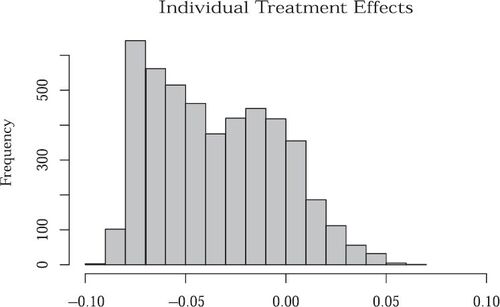
Individual treatment effects estimates are displayed in Figure 2.³¹ The histogram contains 4694 values which represent the effect of literacy on economic outcome for each individual in the sample. Note that even under this different (nonlinear) model specification, the majority of ITEs are negative, indicating that increasing literacy decreases economic outcome for the majority of individuals in the sample. This finding is in line with the average treatment effect estimate in Section 3.3. The spread of the ITE distribution also suggests there is heterogeneity in the effect: the effect of literacy on economic outcome differs across individuals. There are two modes of the ITE distribution; one exists around the linear estimate, –0.05, and the other exists around 0. This implies there are individuals for which literacy does not materially affect economic outcome and others for which it negatively affects economic outcome. Are there traits that distinguish membership in either group? We focus on three variables: household income, gender and education.³²

Fig. 2 The distribution across observations of the estimated individual treatment effects (ITEs). Specifically, each ITE represents the effect of literacy on economic outcome uniquely for each observation in the sample (since N = 4694, there are 4694 values in the above histogram). Similar to the linear treatment effect estimate, the ITEs are collected around negative values, although there are some greater than zero. The spread of this distribution suggests that there is heterogeneity in the effect of literacy on economic outcome.

Figure 3 displays the plot of the ITE distribution for financial literacy by household income, NFCS variable A8. The horizontal axis displays the categories of household income, with a value of 1 indicating an income lower than $15,000 and sequentially higher horizontal axis values related to sequentially higher income amount categories. Category 8 denotes a household income greater than $150,000. The vertical axis displays the ITE distribution for each income category: the black dot is the median ITE, the black line is the 90% interval, and the gray area is the inner quartile range of the distribution.

Fig. 3 Individual treatment effect distributions categorized by the A8 variable, which measures the approximate household annual income. The value “1” denotes less than $15,000, and the value “8” denotes greater than $150,000. The numbers in between are annual incomes of increasing amounts. The black dot denotes the median ITE value within each income category, the black line is the 90% interval of the distribution, and the gray area is the inner quartile range of the distribution.

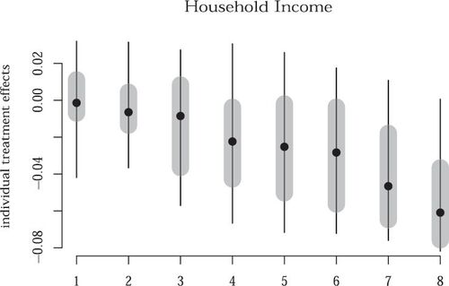
Among the lowest income groups there is no meaningful effect of financial literacy on economic outcome, and that among highest income groups (A8 values from 6 to 8), the effect of literacy on economic outcome monotonically moves to higher negative values. The implication is important for it offers caution about whether resources used to enhance financial literacy offer the benefit of perceived economic comfort. Lower income individuals, whether more financially literate or not, may be able to cover their debt obligations and be satisfied with their level of debt and personal financial condition. Similarly, high income individuals who are financially literate can be dissatisfied with their current economic state and more financial education will not change this perception. While higher incomes and more wealth are preferred generally, our findings suggest that higher levels of financial literacy decrease an individual’s satisfaction with their economic outcome across the household income ranges. We may not yet completely understand why higher income, financially literate individuals have less satisfaction with their economic outcome than their less literate counterparts, but we know that more financially literacy is not causing a higher economic outcome.

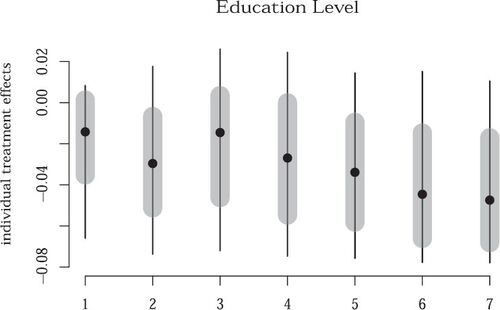
In addition to income levels, we explored gender and education. Figures 4 and 5 show the medians and distributions of individual treatments for gender and education level, respectively. As is apparent in Figure 4, there is no immediate difference between the effect of literacy on economic outcome by gender. Ranges of the literacy parameter within a gender category are similar for both gender categories. Any role that gender might play in how financial literacy impacts economic outcome is de minimis. Differences in education level offer a similar conclusion. The median difference between holders of graduate degrees and those respondents who are less educated exist, however, the distributions of the estimated literacy parameter among individuals within a specific educational classification range widely, thus, across educational classifications there is much overlap indicating that differences are statistically implausible.

Fig. 4 Individual treatment effect distributions for the A3 variable where gender is defined by the value “1” for male and “2” for female.

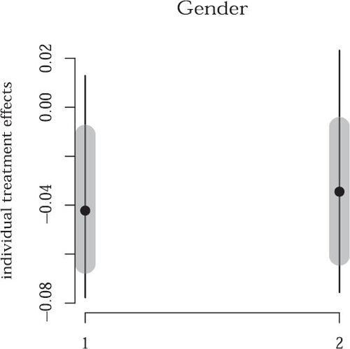
Fig. 5 Individual treatment effect distributions for the A5_2015 variable with categories by education level. The value “1” denotes Did not complete high school, “2” denotes High school graduate—regular high school diploma, “3” denotes High school graduate—GED or alternative credential, “4” denotes Some college, no degree, “5” denotes Associate’s degree, “6” denotes Bachelor’s degree, and “7” denotes Post graduate degree.

While heterogeneity of the financial literacy treatment exists for certain individual characteristics, the more nuanced findings of ITEs still support the general conclusion that more financial literacy offers little measurable economic benefit. Different levels of income, gender and education level do not reveal alternative statistical inferences for the literacy treatment and the NFCS data. Other characteristics within the NFCS datasets may be of interest to literacy researchers, and the modeling approach illustrated in this article charts out an interesting path for future work.

4 Conclusion

Although there is a general consensus that financial literacy is important to households, this article addresses the question of whether financial literacy is causally related to the perceived economic outcomes of individuals. The negative treatment effect does not support the proposition that more financial literacy is necessary to achieve a higher level of perceived economic happiness. Being more financially literate does not increase perceived economic well-being and the finding is robust across income, education and gender subgroups. While economic happiness can be tied to numerous factors, the result from our analysis is that financial literacy is not one of them, and our results corroborate the findings of Netemeyer et al. (2018) in the wellness literature. This finding helps to inform policymakers about required financial educational initiatives such as expanded K-12 education. The cost of efforts to supply financial knowledge may not be valued by individuals and households over the long-run. If the intent of mandated financial literacy education is to raise a household’s future economic outcome, then the result of such expenditures is not promising when the result is not linked to higher perceived economic happiness. Resources may be better spent on other initiatives to achieve such a goal. Lastly, the findings in this article are attributed to the application of a relatively new statistical technique that will help future financial literacy researchers to mitigate bias in their studies while drawing well-grounded causal inferences.

Acknowledgments

We are grateful for Annamaria Lusardi, Brigitte Madrian and Carly Urban’s helpful comments on earlier drafts.

Disclosure Statement

The authors report there are no competing interests to declare.

Notes

1 As an example of financial education sources the CFPB has a consumer tool tab and the U.S. Treasury department has compiled a list. The Chicago FED lists educational offerings of banks in the system.

2 The life-cycle of savings literature has given insight to why people save, spend and borrow, yet professional personal finance advice is driven by rules of thumb, for example, “‘everybody should save 10% of their periodic earnings for retirement.” See Modigliani and Brumberg (1954) and Friedman (1957).

3 Households and individuals can be financially well without being financially literate. They may rely on CPAs for their taxes, a bank relationship for transactions, or financial advisors for investments and insurance products. Moreover, wealthier households may be able and more interested in off-loading financial matters to others and neither care nor are able to answer successfully the standard set of questions that measure financial literacy.

4 See Hastings, Madrian, and Skimmyhorn (2013), pp. 358.

5 Netemeyer et al. (2018) supplemented their work with a measure of overall well-being developed by Su, Tay, and Diener (2014).

6 As noted by Lusardi and Mitchell (2014), p. 34, “Though it is challenging to establish a causal link between financial literacy and economic behavior, both instrumental variables and experimental approaches suggest that financial literacy plays a role in influencing financial decision making, and the causality goes from knowledge to behavior.” Two noteworthy contributions along this path are Calvet, Campbell, and Sodini (2007) and Agarwal et al. (2009)

7 Indeed, most empirical questions surrounding financial literacy are characterized by these problems.

8 These authors propose jointly modeling the treatment and response $Y,Z|\mathrm{X}$ by first modeling the treatment variable as a function of covariates $Z|\mathrm{X}$, and then modeling the response $Y|Z,\mathrm{X}$. The first likelihood provides information on the propensity of being treated as a function of covariates, and the second uses this information to mitigate endogeneity when estimating the partial effect of Z on Y. Importantly, their procedure provides a way to “shrink-away” irrelevant covariates using Bayesian shrinkage priors.

9 In Appendix A, we visually compare our NFCS sample to the entire survey universe to confirm the sample and universe are similar across several covariates.

10 Odean (1998) defined the disposition effect as the tendency for investors who hold losers to hold them too long, and investors who own winners to have sold them too quickly.

11 Choi, Laibson, and Madrian (2011) sample included employees who were older than 59.5 who were unconstrained by withdrawal penalties: they could have simply withdrew employer contributions but chose not to take advantage of it. Even among a subsequent experiment, the researchers find conclude that low financial literacy and poor choice about a matching contribution are positively related.

12 See Survey of the States, Council for Economic Education.

13 Mangrum (2019) explored student loan repayment behavior after college using university-level data from the College Scorecard database. Universities are populated with students from different states, therefore, different financial education experiences, and Mangrum found that “mandated students” improve financial student loan repayment percentages among first generation and low income borrowers.

14 See Willis (2008), p. 204. Willis interprets policymakers’ promotion of financial literacy as an ineffective substitute for financial regulation that places too high a burden on non-expert consumers.

15 See Willis (2011) p. 429.

16 Willis (2011) notes that empirical work to date is replete with evidence that “biases, heuristics, and other non-rational influences” circumvent good financial decision-making. In this study, we are unable to test a hypothesis related specifically to financial education because the 2015 NFCS study did not survey that question.

17 Lusardi, Michaud, and Mitchell (2017), p. 473.

18 Almenberg and Dreber (2015) linked financial literacy and investing in the stock market with the intent to explore how investing varies between men and women when financial literacy is controlled. The authors’ measure financial literacy by identifying basic and advanced financial skills. While the authors find that men have higher probabilities of investing in the stock market, controlling for financial literacy skills reduces the probability differences between men and women substantially, and makes a “gender gap,” inconsequential.

19 53.4% of Balasubramnian and Brisker’s sample used one of the defined advisers.

20 Generally, the economic outcome for a household at any point in time is its economic net worth; that is, assets including household human capital less debt.

21 Studies were conducted in 2009, 2012, 2015, and 2018. See http://www.usfinancialcapability.org.

22 There are 27,564 and 27,091 observations from the surveys conducted in 2015 and 2018, respectively.

23 We will discuss in the empirical analysis below why this is important for inferring a more accurate causal effect estimate and how regularization provides a greater degree of confidence the estimate.

24 The attributes of the final dataset are available from the authors upon request.

25 The interest rate, inflation and risk questions were designed by Olivia Mitchell and Annamaria Lusardi. See Lusardi and Mitchell (2014). According to the 2015 NFCS national report, the Rule of 72 question was added as an additional interest rate question to “to test the concept of interest compounding in the context of debt.”

26 In the NFCS study, the financial investment question is item B14 where an answer of “yes” is coded as a 1 and an answer of “no” a 2.

27 See http://www.usfinancialcapability.org/results.php?region=US.

28 For example, a person who is not satisfied with her current personal financial condition (Question 1) is also likely to have difficulty paying bills every month (Question 2).

29 Several recent studies develop methods for inferring causal effects using machine learning techniques. Chernozhukov et al. (2016) propose a double machine learning approach. Hill (2011) provide an early method using Bayesian Additive Regression Trees. Taddy et al. (2016) and Hahn, Murray, and Carvalho (2020) develop more recent Bayesian approaches for experimental and observational data, respectively. Wager and Athey (2018) provide theoretical guarantees for an approach based on random forests, but Hahn, Murray, and Carvalho (2020) point out the challenges with their method in practice. Little guidance is given for controlling the level of statistical regularization of the random forests, and these practical issues are manifest for any ML method used for causal inference.

30 Hahn et al. (2018) discussed how naive regularization of γ and β in Model 3 will lead to significant bias in the estimate of α—a phenomena called regularization-induced confounding (RIC). To avoid this, we follow an approach outlined in Hahn, Murray, and Carvalho (2020) to control for a prediction of literacy as a function of the covariates. First, we estimate literacy $\widehat{Z}$ from the selection equation in Model 3 with a shrinkage prior placed on the coefficient vector γ. Second, we control for this prediction $\widehat{Z}$ in the response equation and only regularize the coefficients β, leaving unregularized α and the coefficient on $\widehat{Z}$. The shrinkage priors used are closely related to the horseshoe priors of Carvalho, Polson, and Scott (2010) and estimation is undertaken using a variant of the elliptical slice sampler developed in Hahn, He, and Lopes (2019) and implemented in the R package bayeslm. 100,000 MCMC draws from the posterior distribution are generated after 10,000 draws are generated as burn-in. 95% intervals for the model estimates are computed as the empirical quantiles of this posterior distribution.

31 We use an the R package Bayesian causal forests – bcf – to fit the nonlinear model which gives estimates of the individual treatment effects. The current model is built for a binary treatment variable, so we use our existing literacy variable and create a binary version by dividing at the median literacy value. Thus, all sample observations with measured literacy larger (smaller) than the median will labeled as a 1 (0) in the new binary literacy variable. The quantile at which we divide literacy does not effect the overall heterogeneity results described.

32 There are, of course, many traits of potential interest limited only in number by the variables in the underlying dataset.

Appendix A:

Sample and Entire Survey Comparison

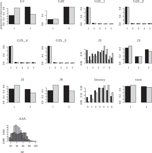
We compare our sample (n = 4694) to the entire survey dataset. Figures 6 and 7 shows the distributions of observations across the covariates used in the analysis for the sample (light gray) and the entire survey dataset (black). There is reasonable balance between the sample and entire survey dataset, suggesting our data sub-setting is not drastically affecting the kinds of observations we use for inference. Pertinent summary statistics of our sample are as follows: respondent age varies from 18 to 86 with an average of 42.6 and a median age of 42. 46% of respondents are female. There is variability in general educational achievement and a skew toward higher educational levels: 10.7% graduated high school with either a diploma or GED, 20.6% completed some college without attaining a degree, 11% and 34% attained associate’s and bachelor’s degrees, respectively, and 23% possessed a post-graduate degree. Variability in household annual income is represented: 7.8% of observations make less than $50,000, 18.2% make less than $75,000, and 74% make greater than $75,000.

Fig. 6 Comparison of sample (light gray) and entire survey datasets across the large set of covariates used for the analysis (first panel).

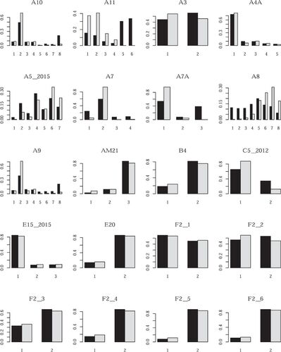
Fig. 7 Comparison of sample (light gray) and entire survey datasets across the large set of covariates used for the analysis (second panel).

References

- Agarwal, S., Ben-David, I., and Yao, V. (2017), “Systematic Mistakes in the Mortgage Market and Lack of Financial Sophistication,” Journal of Financial Economics, 123, 42–58. DOI: 10.1016/j.jfineco.2016.01.028.
- Agarwal, S., Driscoll, J. C., Gabaix, X., and Laibson, D. (2009), “The Age of Reason: Financial Decisions Over the Life Cycle and Implications for Regulation,” Brookings Papers on Economic Activity, 2009, 51–117.
- Almenberg, J., and Dreber, A. (2015), “Gender, Stock Market Participation and Financial Literacy,” Economics Letters, 137, 140–142. DOI: 10.1016/j.econlet.2015.10.009.
- Balasubramnian, B., and Brisker, E. R. (2016), “Financial Adviser Users and Financial Literacy,” Financial Services Review, 25, 127–155.
- Brown, M., Grigsby, J., Van Der Klaauw, W., Wen, J., and Zafar, B. (2016), “Financial Education and the Debt Behavior of the Young,” The Review of Financial Studies, 29, 2490–2522. DOI: 10.1093/rfs/hhw006.
- Calcagno, R., and Monticone, C. (2015), “Financial Literacy and the Demand for Financial Advice,” Journal of Banking & Finance, 50, 363–380.
- Calvet, L. E., Campbell, J. Y., and Sodini, P. (2007), “Down or Out: Assessing the Welfare Costs of Household Investment Mistakes,” Journal of Political Economy, 115, 707–747. DOI: 10.1086/524204.
- Calvet, L. E., Campbell, J. Y., and Sodini, P. (2009), “Measuring the Financial Sophistication of Households,” American Economic Review, 99, 393–398. DOI: 10.1257/aer.99.2.393.
- Campbell, J. Y. (2016), “Restoring Rational Choice: The Challenge of Consumer Financial Regulation,” American Economic Review, 106, 1–30. DOI: 10.1257/aer.p20161127.
- Carvalho, C. M., Polson, N. G., and Scott, J. G. (2010), “The Horseshoe Estimator for Sparse Signals,” Biometrika, 97, 465–480. DOI: 10.1093/biomet/asq017.
- Chernozhukov, V., Chetverikov, D., Demirer, M., Duflo, E., Hansen, C., and Newey, W. K. (2016), “Double Machine Learning for Treatment and Causal Parameters,” Technical report, cemmap working paper.
- Choi, J. J., Laibson, D., and Madrian, B. C. (2011), “$100 Bills on the Sidewalk: Suboptimal Investment in 401 (k) Plans,” Review of Economics and Statistics, 93, 748–763. DOI: 10.1162/REST_a_00100.
- Friedman, M. (1957), “The Permanent Income Hypothesis,” in A Theory of the Consumption Function, pp. 20–37, Princeton, NJ: Princeton University Press.
- Hahn, P. R., Carvalho, C. M., Puelz, D., and He, J. (2018), “Regularization and Confounding in Linear Regression for Treatment Effect Estimation,” Bayesian Analysis, 13, 163–182. DOI: 10.1214/16-BA1044.
- Hahn, P. R., He, J., and Lopes, H. F. (2019), “Efficient Sampling for Gaussian Linear Regression with Arbitrary Priors,” Journal of Computational and Graphical Statistics, 28, 142–154. DOI: 10.1080/10618600.2018.1482762.
- Hahn, P. R., Murray, J. S., and Carvalho, C. M. (2020), “Bayesian Regression Tree Models for Causal Inference: Regularization, Confounding, and Heterogeneous Effects,” (with Discussion), Bayesian Analysis, 15, 965–1056.
- Harvey, M. (2019), “Impact of Financial Education Mandates on Younger Consumers’ Use of Alternative Financial Services,” Journal of Consumer Affairs, 53, 731–769. DOI: 10.1111/joca.12242.
- Hastings, J. S., Madrian, B. C., and Skimmyhorn, W. L. (2013), “Financial Literacy, Financial Education, and Economic Outcomes,” Annual Review of Economics, 5, 347–373. DOI: 10.1146/annurev-economics-082312-125807.
- Hill, J. L. (2011), “Bayesian Nonparametric Modeling for Causal Inference,” Journal of Computational and Graphical Statistics, 20, 217–240. DOI: 10.1198/jcgs.2010.08162.
- Imbens, G. W., and Rubin, D. B. (2015), Causal Inference in Statistics, Social, and Biomedical Sciences, Cambridge: Cambridge University Press.
- Keys, B. J., Pope, D. G., and Pope, J. C. (2016), “Failure to Refinance,” Journal of Financial Economics, 122, 482–499. DOI: 10.1016/j.jfineco.2016.01.031.
- Leamer, E. E. (1978), Specification Searches: Ad hoc Inference with Nonexperimental Data (Vol. 53), New York: Wiley.
- Leamer, E. E. (1983), “Let’s Take the Con Out of Econometrics,” The American Economic Review, 73, 31–43.
- Lusardi, A., Michaud, P.-C., and Mitchell, O. S. (2017), “Optimal Financial Knowledge and Wealth Inequality,” Journal of Political Economy, 125, 431–477. DOI: 10.1086/690950.
- Lusardi, A., and Mitchell, O. S. (2014), “The Economic Importance of Financial Literacy: Theory and Evidence,” Journal of Economic Literature, 52, 5–44. DOI: 10.1257/jel.52.1.5.
- Lusardi, A., Mitchell, O. S., and Oggero, N. (2020), “Debt and Financial Vulnerability on the Verge of Retirement,” Journal of Money, Credit and Banking, 52, 1005–1034. DOI: 10.1111/jmcb.12671.
- Mangrum, D. (2019), “Personal Finance Education Mandates and Student Loan Repayment,” Available at SSRN 3349384.
- Mitchell, O. S., and Lusardi, A. (2015), “Financial Literacy and Economic Outcomes: Evidence and Policy Implications,” The Journal of Retirement, 3, 107–114. DOI: 10.3905/jor.2015.3.1.107.
- Modigliani, F., and Brumberg, R. H. (1954), “Utility Analysis and the Consumption Function: An Interpretation of Cross-Section Data,” Post Keynesian Economics, Rutgers University Press, New Brunswick, pp. 388–436.
- Netemeyer, R. G., Warmath, D., Fernandes, D., and Lynch Jr, J. G. (2018), “How Am I Doing? Perceived Financial Well-Being, its Potential Antecedents, and its Relation to Overall Well-Being,” Journal of Consumer Research, 45, 68–89. DOI: 10.1093/jcr/ucx109.
- Odean, T. (1998), “Are Investors Reluctant to Realize their Losses?” The Journal of Finance, 53, 1775–1798. DOI: 10.1111/0022-1082.00072.
- Stoddard, C., and Urban, C. (2020), “The Effects of State-Mandated Financial Education on College Financing Behaviors,” Journal of Money, Credit and Banking, 52, 747–776. DOI: 10.1111/jmcb.12624.
- Su, R., Tay, L., and Diener, E. (2014), “The Development and Validation of the Comprehensive Inventory of Thriving (cit) and the Brief Inventory of Thriving (bit),” Applied Psychology: Health and Well-Being, 6, 251–279.
- Taddy, M., Gardner, M., Chen, L., and Draper, D. (2016), “A Nonparametric Bayesian Analysis of Heterogenous Treatment Effects in Digital Experimentation,” Journal of Business & Economic Statistics, 34, 661–672.
- Urban, C., Schmeiser, M., Collins, J. M., and Brown, A. (2018), “The Effects of High School Personal Financial Education Policies on Financial Behavior,” Economics of Education Review, 78, 101786. DOI: 10.1016/j.econedurev.2018.03.006.
- Wager, S., and Athey, S. (2018), “Estimation and Inference of Heterogeneous Treatment Effects Using Random Forests,” Journal of the American Statistical Association, 113, 1228–1242. DOI: 10.1080/01621459.2017.1319839.
- Willis, L. E. (2008), “Against Financial-Literacy Education,” Iowa Law Review, 94, 197–285.
- Willis, L. E. (2011), “The Financial Education Fallacy,” American Economic Review, 101, 429–34.