Marginal Structural Models to Estimate Causal Effects of Right-to-Carry Laws on Crime

Abstract

Right-to-carry (RTC) laws allow the legal carrying of concealed firearms for defense, in certain states in the United States. I used modern causal inference methodology from epidemiology to examine the effect of RTC laws on crime over a period from 1959 up to 2016. I fitted marginal structural models (MSMs), using inverse probability weighting (IPW) to correct for criminological, economic, political and demographic confounders. Results indicate that RTC laws significantly increase violent crime by 7.5% and property crime by 6.1%. RTC laws significantly increase murder and manslaughter, robbery, aggravated assault, burglary, larceny theft and motor vehicle theft rates. Applying this method to this topic for the first time addresses methodological shortcomings in previous studies such as conditioning away the effect, overfit and the inappropriate use of county level measurements. Data and analysis code for this article are available online.

Keywords:

• Causal modeling
• Concealed carry
• Firearms
• Gun laws
• Inverse probability weighting
• Longitudinal data
• Marginal structural model
• Multiple imputation
• Random effects

1 Introduction

Lott and Mustard (1997) concluded that the introduction of right-to-carry (RTC) laws in states in the United States decreases violent crime. These laws allow the legal carrying of concealed firearms for self-defense. Since then, many studies (see Section 5) have been conducted on this issue, with conflicting results. For example, Donohue, Aneja, and Weber (2019) concluded that RTC laws substantially increase violent crime. As described in Lott and Mustard (1997), Lott (2010), and Donohue, Aneja, and Weber (2019) RTC laws could simultaneously both have a positive effect (e.g., by deterrence) and a negative effect (e.g., by escalation or displacement) on crime.

The National Research Council (U.S.) (2004) concluded that to reach a robust scientifically supported conclusion, new analytical approaches are needed. For example, as described in Section 5, many methods typically used in previous studies can suffer from adjusting away the effect, overfitting and inappropriate use of county level measurements, among others. In this article, I attempt to address these deficiencies using marginal structural models (MSMs), a causal inference technique popular in epidemiology (Hernán, Brumback, and Robins 2000; Robins, Hernán, and Brumback 2000; Hernán and Robins 2006a).

2 Background: Marginal Structural Models (MSMs)

MSMs are used in epidemiology to estimate the causal effect of a treatment on a chosen outcome in medical patients, from observational data (Robins, Hernán, and Brumback 2000; Hernán, Brumback, and Robins 2000; Hernán and Robins 2006a). I introduce the theory of MSMs and illustrate their advantages over standard models below.

MSMs are based on the concept of counterfactuals, also called potential outcomes (Robins 1999; Höfler 2005). Counterfactuals are the outcomes that could have been observed, had a certain exposure been applied to an observational unit. For instance, the outcome after exposure to a medical treatment of patients, or the outcome after the introduction of RTC laws in states in the United States. Causal effects can then be defined as contrasts between these potential outcomes (Hernán 2004; Hernán and Robins 2006a).

For example, consider patients receiving either a medical treatment or a placebo in a clinical trial. The outcome Y could be survival (yes or no). With dichotomous exposure A, the potential outcome for individual i when receiving treatment level 0, the placebo is $Y_{i,a=0}$. The potential outcome for individual i when receiving treatment level 1, the medical treatment is $Y_{i,a=1}$. The causal effect of the medical treatment on survival, as compared to the placebo, for individual i could then be expressed as the difference between $Y_{i,a=0}$ and $Y_{i,a=1}$.

At the population level, the causal effect of a dichotomous exposure A on an outcome Y can be defined as a contrast between distributions of potential outcomes. The distribution of outcomes when every observational unit would have received exposure level 0 is $f(y_{a=0})$. The distribution of outcomes when every unit would have received exposure level 1 is $f(y_{a=1})$. The causal effect comparing these two distributions could be expressed for instance as a difference or ratio of the survival rates. Such a contrast is referred to as a marginal causal effect. This is precisely the effect that is desired when estimating the causal effect of a specific action, treatment or policy, such as when estimating the effect of RTC laws on crime (Hernán 2004).

2.1 Marginal Structural Models (MSMs)

Using the counterfactual framework, the marginal causal effect of an exposure on a chosen outcome can be described quantitatively using a MSM (Hernán, Brumback, and Robins 2000; Robins, Hernán, and Brumback 2000; Hernán and Robins 2006a). For example, the MSM(1) $$E(Y_a)={\beta }_0+{\beta }_{1}a$$(1) could describe the causal effect of a dichotomous exposure A on a continuous outcome Y. The response variable Y_a is the potential outcome that would have been observed, when every unit of observation would have received the same specific treatment level a. Parameter β₁ then quantifies the causal effect of A on Y. This parameter is equal to the difference in the mean of Y between the distributions of the potential outcomes corresponding to the two treatment levels of A, $f(y_{a=0})$ and $f(y_{a=1})$. The parameters of such a MSM could be estimated by fitting the standard regression model(2) $$E(Y)={\beta }_0+{\beta }_{1}A$$(2) on observations $\{Y_i,A_i\}$ from a randomized experiment with no selection bias. However, in observational studies bias due to confounding is often present, as described in the next paragraph.

2.2 Confounding

Confounding occurs when one or more covariates have a causal effect both on the exposure allocation and on the outcome (Pearl 2009). Such covariates are referred to as “confounders.” An example of a confounder in a medical setting is disease progression in HIV positive individuals, when estimating the effect of treatment on mortality. Disease progression could both affect the start of treatment as well as mortality (Hernán, Brumback, and Robins 2000). Or, in the present study, for example the composition of the state legislature could possibly affect both the introduction of RTC laws as well as crime rates, either directly or indirectly. Unadjusted effect estimators such as Equation (2)(2) $$E(Y)={\beta }_0+{\beta }_{1}A$$(2) are biased estimators of the causal effect when confounding is present (Greenland and Morgenstern 2001). Adjusting for confounding is possible using various methods. I will describe both traditional “conditional” regression models in which confounders are included as covariates, and inverse probability weighting (IPW) to correct for confounding while fitting a MSM.

2.3 Conditional Models and their Drawbacks

The most commonly used statistical method to adjust for confounding is conditioning, as was indeed done in previous studies on the effect of RTC laws on crime (Section 5). Conditioning amounts to the pooling of associations, estimated within strata defined by confounders. In this manner, an overall adjusted effect estimate is obtained. Such a pooled estimate can be obtained by using stratification methods, or by including confounders as covariates in regression models (Fitzmaurice 2004; Ranstam 2008).

A drawback of conditioning is that effects can be adjusted away, especially in a longitudinal setting. I will illustrate this in the context of estimating the effect of RTC laws on crime. I indicate time in years since a chosen baseline using j. Consider the time-varying exposure A_j , the implementation of a RTC law at the state level (0 = no, 1 = yes). Also, consider violent crime rate Y_j at the state level, and the composition of the state legislature L_j . The effect of A_j on Y_j could be confounded by time-varying covariate L_j . I illustrate this temporal structure at time points j and j – 1 in Figure 1 using a directed acyclic graph (DAG) (Hernán, Hernández-Díaz, and Robins 2004; Hernán and Robins 2006b). DAGs illustrate the assumed causal structure between variables, with nodes representing variables, and causal effects depicted by unidirectional edges (arrows).

Fig. 1 Illustration of the temporal structure between a (possible) confounder such as state legislature composition L, RTC law implementation A and the crime rate Y at two subsequent time points j – 1 and j. Confounding is indicated by $\star$. By conditioning on L, the indirect effect of A on Y through L, as indicated by ⋆⋆, is adjusted away.

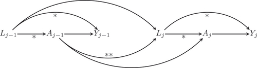
Suppose that state legislature composition L_j is a confounder for the effect of A_j on Y_j , assuming it has a causal effect on both A_j and Y_j , as indicated by $\star$. Assuming that the implementation of a RTC law at a given time point also has an effect on the composition of the state legislature at a subsequent time point (the effect of $A_{j-1}$ on L_j ), $A_{j-1}$ has an indirect effect on Y_j through L_j , as indicated by ⋆⋆. When “adjusting” for the state legislature composition in the previous year by including it as a covariate in a regression model, the indirect effect of RTC laws on crime is adjusted away (Robins 1997; Robins, Greenland, and Hu 1999).

The problem of adjusting away the effect will occur when conditioning on any variable that is also intermediate for the effect of the exposure. This can occur when estimating the effect of RTC laws on crime, when including possible longitudinal confounders in the regression model, as was done in previous studies on this topic. The association will still be a biased estimate of the true causal effect.

Other drawbacks of conditional regression models include non-collapsibility and collider stratification, which can both introduce more bias. Non-collapsibility entails that effect estimates from conditional models are only true estimates of marginal effects with a model that uses a linear or log-linear link function (Greenland, Robins, and Pearl 1999). Collider stratification is the introduction of bias by conditioning on a common effect of two variables. This can also occur in the longitudinal situation illustrated in Figure 1. For a more detailed explanation I refer to the literature (Greenland 2003; Whitcomb et al. 2009).

In this article, I use inverse probability weighting (IPW) to address some of the limitations of conditional modeling, as explained below.

2.4 Introduction to Inverse Probability Weighting (IPW)

The parameters of MSMs can be estimated using IPW to correct for confounding (Robins 1998). Fitting a MSM using IPW amounts to weighting each observation by the inverse of the probability of the observed exposure level, given the observed value of the confounders. Subsequently, a MSM regressing the outcome on the exposure is fitted on the weighted dataset. I illustrate this in a point treatment study (i.e., at one specific time point) below, and generalize to a longitudinal setting in Section 3.4.

Consider a point treatment setting with a dichotomous exposure A, outcome Y and a vector of possible confounders K measured at a single time point. Using IPW, we can adjust for confounders K by weighting each observation i by the inverse probability weight(3) $$w_i=\frac{1}{\mathrm{P}(A_i=a_i|{\mathit{K}}_i={\mathit{k}}_i)}.$$(3)

I indicate the observed exposure and confounder status with a and k, respectively. The denominator of Equation (3)(3) $$w_i=\frac{1}{\mathrm{P}(A_i=a_i|{\mathit{K}}_i={\mathit{k}}_i)}.$$(3) contains the probability of the observed exposure level given the observed values of confounders K. The denominator can be estimated from a model regressing $\mathrm{P}(A=1)$ on K, either using the predicted probability or one minus the predicted probability, for a_i = 1 and a_i = 0, respectively. Weighting by w_i creates a pseudo-population in which K no longer predicts A, but in which the causal effect of A on Y is still present (Robins 1998). Weighting observations i by w_i one can then fit a model such as Equation (2)(2) $$E(Y)={\beta }_0+{\beta }_{1}A$$(2) to estimate the parameters of MSM Equation (1)(1) $$E(Y_a)={\beta }_0+{\beta }_{1}a$$(1) .

To increase statistical efficiency and attain better coverage of confidence intervals, it is recommended to use stabilized weights (Hernán, Brumback, and Robins 2000; Cole and Hernán 2008), for example,(4) $$s{w}_i=\frac{\mathrm{P}(A_i=a_i)}{\mathrm{P}(A_i=a_i|{\mathit{K}}_i={\mathit{k}}_i)}.$$(4)

The numerator of Equation (4)(4) $$s{w}_i=\frac{\mathrm{P}(A_i=a_i)}{\mathrm{P}(A_i=a_i|{\mathit{K}}_i={\mathit{k}}_i)}.$$(4) contains the probability of the observed exposure level, which can be estimated using the observed proportions. To further stabilize the weights, one can condition both in the numerator and in the denominator of Equation (4)(4) $$s{w}_i=\frac{\mathrm{P}(A_i=a_i)}{\mathrm{P}(A_i=a_i|{\mathit{K}}_i={\mathit{k}}_i)}.$$(4) on a set of covariates V that are not confounders.

2.5 Assumptions

The following assumptions are made when fitting a MSM using IPW (Cole and Hernán 2008). The assumption of consistency states that the counterfactual outcome corresponding to the observed exposure level is precisely the observed outcome (Robins, Greenland, and Hu 1999; Cole and Hernán 2008). This means that the exposure, the causal effect of which is to be estimated, needs to be clearly defined. It is also necessary to assume positivity, which means that every level of the exposure of interest has a positive probability of being allocated in every stratum defined by the measured confounders (Cole and Hernán 2008; Petersen et al. 2012). This assumption is also known as the assumption of experimental treatment assignment (ETA). The assumption of conditional exchangeability means that within strata defined by the measured confounders, potential outcomes are independent of the observed exposure level (Hernán and Robins 2006a). In practice, this holds when there are no unmeasured confounders.

3 Methods

I have estimated the causal effect of the adoption of RTC laws in states in the United States on crime rates with a MSM for each crime type, correcting for confounding using IPW. I combined this method with multiple imputation to deal with missing values. Below I describe the details of this method. I have implemented the described method in the R software (R Core Team 2021), version 4.0.5. I have made the data and statistical code available with this article, for full transparency and falsifiability, and to allow researcher to improve upon this analysis as they see fit (see supplementary materials).

3.1 Data

Observational units i are all 50 states in the United States, with measurements taken in calendar years $T_j=1959,1960,\dots ,2016$, with $j=0,1,\dots ,57$ corresponding to those 58 calendar years, respectively. I have chosen to start the follow up at 1959 since that is when the first RTC law was implemented, in New Hampshire (Donohue, Aneja, and Weber 2019). I included the following variables in the dataset:

Total reported numbers of crimes $Y_{ij}^c$ in each state i, at the end of each year j, with $c=1,2,\dots ,9$ representing violent crime total, murder/manslaughter, forcible rape, robbery, aggravated assault, property crime total, burglary, larceny theft and motor vehicle theft, respectively. These variables as well as total state population P_ij were obtained from Federal Bureau of Investigation (2019c) for 1960 up to 2014 for most states and for 1965 up to 2014 for the state of New York. $Y_{ij}^c$ and P_ij data for all states in 2015 and 2016 were obtained from Federal Bureau of Investigation (2019a) and Federal Bureau of Investigation (2019b), respectively. Corresponding crime rates can be computed from $Y_{ij}^c$ and P_ij . Measurements for these variables were missing for the state of New York in 1959 up to 1964 and in 1959 for the other states.

I have also used RTC law implementation A_ij with $0=$ restrictive (no-issue or may-issue) and $1=$ permissive (shall-issue or unrestricted) according to Donohue, Aneja, and Weber (2019). A_ij = 1 for the years in which a RTC law was in effect for the majority of that year, and A_ij = 0 otherwise.

I have collected possible longitudinal confounders for the effect of RTC laws on crime in vector ${\mathit{L}}_{ij}$ including the following. I used the state violent crime rate and property crime rate per 100.000 people, as computed above, at the end of year j – 2. Since this variable is measured at the end of year, I have used a lag of two years to satisfy proper temporal ordering, as illustrated in Figure 1. This necessitated state level measurements of this variable from 1957 up to 2014. Measurements for these variables were missing for the state of New York in 1957 up to 1964 and in 1957, 1958, and 1959 for the other states.

I also included the state share of the total U.S. Gross Domestic Product (GDP), at the end of year j – 2 to satisfy proper temporal ordering. This necessitated state level measurements for this variable from 1957 up to 2014. I obtained measurements from 1963 up to 2014 for every state from Bureau of Economic Analysis (2019), therefore, the variable had missing values for 1957 up to 1962. To improve normality, I used a natural logarithm transformation.

As possible confounders I also used various demographic variables including the proportions of the population that is female, white non-hispanic, and of age between 0–18, 19–39, and 40–64 (with 65 and above redundant), respectively. Since these variable are measured at the end of year, I employed a lag of two years necessitating measurements from 1957 up to 2014. I computed these proportions from population counts by sex, race and age obtained from different tables including US Census Bureau (2017a, 2017b, 2019a, 2019b, 2019c, 2019). These population counts also included measurements for 1950 which I used to add further support to the multiple imputation model described in Section 3.2. Values for 1957, 1958, 1959, and 1961 up to 1969 were missing.

I used Population density computed from the population counts P_ij and the state land areas in square miles obtained from US Census Bureau (2016). These were transformed using a natural logarithm to improve normality, and lagged by two years for similar reasons as the demographic variables.

As possible confounders I also included an indicator variable indicating that the state legislation has a Republican majority, measured at the beginning of the previous year, to satisfy temporal ordering according to Figure 1. I used data from Klarner (2013) and National Conference of State Legislatures (NCSL) (2019), before and from 1978 onwards, respectively. And I also used an indicator variable indicating that the state governor is a Republican, measured at the beginning of the previous year, to satisfy temporal ordering according to Figure 1. I used data from Klarner (2013) and National Conference of State Legislatures (NCSL) (2019), before and from 2009 onwards, respectively. The interaction between the indicator variables for the state legislation and state governor party was also included.

I assumed that the above included criminological, economic, political and demographic possible confounders all are likely to affect both the implementation of a RTC law and crime rates, just like variable L in Figure 1 with j representing follow-up time in years. The temporal ordering in Figure 1 is always satisfied since I used a lag of one year for confounders measured at the beginning of the year and a lag of two years for confounders measured at the end of the year.

I have used natural splines (De Boor 2001) with three degrees of freedom fitted on calendar time and follow-up time in the imputation model (Section 3.2), the main MSM models (Section 3.3) and the models for the implementation of a RTC law (Section 3.4). A natural spline with three degrees of freedom has two boundary knots and one interior knot, so that within two distinct periods different cubic trends can be fitted. I consider this choice sufficiently flexible to model calendar year in the context of crime rates and RTC law implementation, based on the observed trend of an increase of crime rates from 1960 up to the “crack era” of the 1980s and 1990s, followed by a decrease. I illustrate this trend in the longitudinal plots in the supplementary materials. I assumed that the relatively limited amount of data does not allow for a more complex model, although I explore varying degrees of freedom in the sensitivity analysis (Section 3.5).

I assessed the positivity assumption (see Section 2.5) graphically, using scatterplots of the implementation of a RTC law (yes/no) against each possible confounder, for each of the multiple imputation datasets that were generated as described below (see supplementary materials).

3.2 Multiple Imputation

To deal with the missing values in the data as described above I performed multiple imputation for multivariate, multilevel data using Markov chain Monte Carlo (MCMC) according to Schafer and Yucel (2002). I used a multivariate linear mixed-effects model to impute the missing values. As dependent variables I used the natural logarithm of the crime numbers, natural logarithm of state population numbers, natural logarithm of the state share of the total U.S. Gross Domestic Product (GDP), the proportions of the population that is female, white non-hispanic, and of age between 0–18, 19–39, and 40–64, respectively. As independent predictors in this model I used the intercept, the indicator for RTC law implementation, a natural spline (De Boor 2001) with three degrees of freedom fitted on calendar year, and a random intercept for each state.

Using 200 MCMC iterations after 5.000 burn-in iterations, I generated 25 imputed datasets from this model. The number of iterations and datasets was chosen based on technical feasibility in the sensitivity analysis as described below. On each of these 25 imputed datasets MSMs for the effect of RTC laws on crime rates were fitted using IPW as described below. Estimates and standard errors were combined according to Rubin’s rules (Rubin 1987). After this, I performed a sensitivity analysis as described in Section 3.5.

3.3 Marginal Structural Models

To model the causal effect of the implementation of RTC laws on crime, for each of the crime types c I have estimated the parameters of a separate generalized linear mixed model (GLMM) (Wolfinger and O’connell 1993), with a quasi-Poisson link function:(5) $$\hspace{0.17em}\log \hspace{0.17em}\left(\frac{\mathrm{E}(Y_{\mathit{aij}}^c)}{P_{ij}}\right)={\theta }_0^c+{\theta }_1^c{a}_{ij}+{\mathit{\theta }}_2^c{\mathit{f}}^1(T_j)+{\xi }_i^c.$$(5)

These models convert the numbers of crimes for each type per state and year $Y_{ij}^c$ to crime rates using the offset P_ij . The models include the effect ${\theta }_1^c$ of the dummy variable for the RTC laws per state, per year, a_ij . The function ${\mathit{f}}^1(T_j)$ indicates a natural spline (De Boor 2001) with three degrees of freedom, as a flexible modeling of calendar time. ${\xi }_i^c$ indicates a normally distributed random intercept at the state level. This approach is somewhat similar to the generalized estimating equation (GEE) model described by eq (1b) in Hernán, Brumback, and Robins (2002), with the addition of the random intercept.

Compared to a standard Poisson link function, the quasi-Poisson link function uses an additional scale parameter allowing for under- or overdispersion of the error distribution (Zeileis, Kleiber, and Jackman 2008). I have also incorporated an autoregressive correlation structure of order one (AR1) (Littell, Pendergast, and Natarajan 2000) between the repeated outcomes of each state. I consider this structure an appropriate choice for repeated measures over time, since the correlation between measurements declines when those measurements are spaced further apart in time (Littell, Pendergast, and Natarajan 2000). While using IPW to correct for confounding as described below, I performed two-sided significance testing at a significance level of 5%, compared to 0 under the null hypothesis for the main effects ${\theta }_1^c$.

The causal effects estimated by ${\theta }_1^c$ can be interpreted in the following manner. The MSMs Equation (5)(5) $$\hspace{0.17em}\log \hspace{0.17em}\left(\frac{\mathrm{E}(Y_{\mathit{aij}}^c)}{P_{ij}}\right)={\theta }_0^c+{\theta }_1^c{a}_{ij}+{\mathit{\theta }}_2^c{\mathit{f}}^1(T_j)+{\xi }_i^c.$$(5) model for each crime rate the contrast between two distributions of potential outcomes: (a) the repeated measurements of the crime rates in each state, when all states would never have implemented a RTC law during follow-up, and (b) the repeated measurements of the crime rates in each state, when all states would have always had a RTC law implemented, during the complete follow-up. This effect is quantified by the parameters ${\theta }_1^c$, from which the risk ratios ${\mathrm{e}}^{{\theta }_1^c}$ can be computed. When such a risk ratio would for example, be equal to 1.1, that should be interpreted as the implementation of a RTC law increasing the corresponding crime rate by 10%, while a risk ratio of 0.9 would equal a decrease by 10%.

3.4 Inverse Probability Weighting

I have fitted model Equation (5)(5) $$\hspace{0.17em}\log \hspace{0.17em}\left(\frac{\mathrm{E}(Y_{\mathit{aij}}^c)}{P_{ij}}\right)={\theta }_0^c+{\theta }_1^c{a}_{ij}+{\mathit{\theta }}_2^c{\mathit{f}}^1(T_j)+{\xi }_i^c.$$(5) on the observed data, for each of the crime types, correcting for confounding by the longitudinal variables in ${\mathit{L}}_{ij}$, using IPW. I have weighted each observation ij by the stabilized weights sw_ij , similarly to Hernán, Brumback, and Robins (2002):(6) $$s{w}_{ij}=\prod _{k=0}^j\frac{\mathrm{P}(A_{ik}=a_{ik}|{\overline{A}}_{ik-1}={\overline{a}}_{ik-1})}{\mathrm{P}(A_{ik}=a_{ik}|{\overline{A}}_{ik-1}={\overline{a}}_{ik-1},{\overline{\mathit{L}}}_{ik}={\overline{\mathit{l}}}_{ik})}.$$(6)

This weight is for each measurement j for each state i the product over all previous time points of a ratio of probabilities. The factors in the numerator contain the probability of the observed exposure status at each time point, a_ij , given the observed exposure history up to the previous time point ${\overline{a}}_{ij-1}=a_{i0},a_{i1},\dots ,a_{ij-1}$. The factors in the denominator contain the probability of the observed exposure status at each time point, a_ij , given the observed exposure history up to the previous time and the observed history of the longitudinal confounders ${\overline{\mathit{l}}}_{ij}={\mathit{l}}_{i0},{\mathit{l}}_{i1},\dots ,{\mathit{l}}_{ij}$.

I have estimated the factors in Equation (6)(6) $$s{w}_{ij}=\prod _{k=0}^j\frac{\mathrm{P}(A_{ik}=a_{ik}|{\overline{A}}_{ik-1}={\overline{a}}_{ik-1})}{\mathrm{P}(A_{ik}=a_{ik}|{\overline{A}}_{ik-1}={\overline{a}}_{ik-1},{\overline{\mathit{L}}}_{ik}={\overline{\mathit{l}}}_{ik})}.$$(6) as follows. The introduction of a RTC law was never reversed in any state. I assumed that after the first instance of having a RTC law within follow up in a specific state, the elements $\mathrm{P}(A_{ik}=a_{ik}|\dots )$ are equal to one. In other words, after the first instance of having a RTC law within follow up, the probability of having a RTC law in that state is always one. Using only the data up to and including the first year in which a RTC law was implemented within follow up, I have estimated the other elements in the denominator of Equation (6)(6) $$s{w}_{ij}=\prod _{k=0}^j\frac{\mathrm{P}(A_{ik}=a_{ik}|{\overline{A}}_{ik-1}={\overline{a}}_{ik-1})}{\mathrm{P}(A_{ik}=a_{ik}|{\overline{A}}_{ik-1}={\overline{a}}_{ik-1},{\overline{\mathit{L}}}_{ik}={\overline{\mathit{l}}}_{ik})}.$$(6) using the regression model(7) $$\hspace{0.17em}\log \hspace{0.17em}(-\hspace{0.17em}\log \hspace{0.17em}(1-\mathrm{P}(A_{ij}=1)))={\beta }_0+{\mathit{\beta }}_1{\mathit{f}}^2(j)+{\mathit{\beta }}_2{\mathit{L}}_{ij}.$$(7)

Model Equation (7)(7) $$\hspace{0.17em}\log \hspace{0.17em}(-\hspace{0.17em}\log \hspace{0.17em}(1-\mathrm{P}(A_{ij}=1)))={\beta }_0+{\mathit{\beta }}_1{\mathit{f}}^2(j)+{\mathit{\beta }}_2{\mathit{L}}_{ij}.$$(7) is similar to a Cox proportional hazards model, but with the outcome observed in discrete time, using the complementary log-log link function (Prentice and Gloeckler 1978). I have included main effects of the longitudinal confounders L, including the interaction between state legislature composition and governor party. The function ${\mathit{f}}^2(j)$ indicates a natural spline with three degrees of freedom fitted on follow up time, as a flexible baseline hazard function. The elements in the numerator of Equation (6)(6) $$s{w}_{ij}=\prod _{k=0}^j\frac{\mathrm{P}(A_{ik}=a_{ik}|{\overline{A}}_{ik-1}={\overline{a}}_{ik-1})}{\mathrm{P}(A_{ik}=a_{ik}|{\overline{A}}_{ik-1}={\overline{a}}_{ik-1},{\overline{\mathit{L}}}_{ik}={\overline{\mathit{l}}}_{ik})}.$$(6) were estimated using a similar model including only ${\mathit{f}}^2(j)$ and the intercept.

As a robustness check, I computed Pearson correlation coefficients between the measured predictors that were included in the models fitted to estimate the weights. I regarded excessively high correlations (i.e., > 0.8) as an indication of possibly problematic multicollinearity in these models. When computing these correlations, I used only the data up to and including the first year in which a RTC law was implemented within follow up, to which these models were fitted, before imputation.

Note that exposure allocation model Equation (7)(7) $$\hspace{0.17em}\log \hspace{0.17em}(-\hspace{0.17em}\log \hspace{0.17em}(1-\mathrm{P}(A_{ij}=1)))={\beta }_0+{\mathit{\beta }}_1{\mathit{f}}^2(j)+{\mathit{\beta }}_2{\mathit{L}}_{ij}.$$(7) uses 16 parameters including the intercept. Given the 42 observed “events” corresponding to the first instance of having a RTC law implemented within follow up (see Section 4), I consider this the maximum acceptable complexity of the model, based on the simulation studies performed by Vittinghoff and McCulloch (2007).

3.5 Sensitivity Analysis

I have performed a sensitivity analysis to examine the robustness of the results. I have fitted the following variations of the main MSMs.

Variants 1–11 each subtract a specific component of the model Equation (7)(7) $$\hspace{0.17em}\log \hspace{0.17em}(-\hspace{0.17em}\log \hspace{0.17em}(1-\mathrm{P}(A_{ij}=1)))={\beta }_0+{\mathit{\beta }}_1{\mathit{f}}^2(j)+{\mathit{\beta }}_2{\mathit{L}}_{ij}.$$(7) : in variant (1) violent crime is dropped from the model, in (2) property crime is dropped, in (3) GDP share, (4) proportion female, (5) proportion white non-hispanic, (6) the age variables, (7) population density, (8) the interaction between the indicator that the state legislature has a Republican majority and the indicator that the state governor is Republican, (9) state legislature, (10) state governor and in (11) both the state legislature and governor indicators are dropped.

In variant (12) I have added to the exposure allocation model specified by Equation (7)(7) $$\hspace{0.17em}\log \hspace{0.17em}(-\hspace{0.17em}\log \hspace{0.17em}(1-\mathrm{P}(A_{ij}=1)))={\beta }_0+{\mathit{\beta }}_1{\mathit{f}}^2(j)+{\mathit{\beta }}_2{\mathit{L}}_{ij}.$$(7) both the two-way interactions and the three way interactions between the spline fitted on follow-up time, the indicator that the state legislature has a Republican majority and the indicator that the state governor is Republican. In this manner, possible paradigm shifts within the Democratic and Republican party are captured. These paradigm shifts could modify the effect of these political variables on the probability that a RTC law is implemented.

As explained in Cole and Hernán (2008), the statistical efficiency of an IPW estimator can be increased by truncating the weights, at the cost of introducing a small amount of bias. When truncating, weights below or above a chosen percentile are set to that percentile, at the lower and upper end of the distribution of the weights, respectively. That is, a one-sided truncation proportion of 0.01 would indicate truncating at the 1st and 99th percentile. In the sensitivity analysis I have included the following variants: (13) weights truncated at the 1st and 99th percentile, (14) weights truncated at the 2nd and 98th percentile and (15) weights truncated at the 5th and 95th percentile.

Both in the exposure allocation model Equation (7)(7) $$\hspace{0.17em}\log \hspace{0.17em}(-\hspace{0.17em}\log \hspace{0.17em}(1-\mathrm{P}(A_{ij}=1)))={\beta }_0+{\mathit{\beta }}_1{\mathit{f}}^2(j)+{\mathit{\beta }}_2{\mathit{L}}_{ij}.$$(7) and the MSMs Equation (5)(5) $$\hspace{0.17em}\log \hspace{0.17em}\left(\frac{\mathrm{E}(Y_{\mathit{aij}}^c)}{P_{ij}}\right)={\theta }_0^c+{\theta }_1^c{a}_{ij}+{\mathit{\theta }}_2^c{\mathit{f}}^1(T_j)+{\xi }_i^c.$$(5) natural splines with three degrees of freedom are used on follow-up time and calendar time, respectively. I examined the sensitivity of the main effect estimates to the number of degrees of freedom. I fitted the following variants: variant (16) with a spline with two degrees of freedom in the exposure allocation model, variant (17) including a spline with four degrees of freedom in the exposure allocation model, variant 18) using a spline with two degrees of freedom in the MSMs and variant (19) using a spline with four degrees of freedom in the MSMs.

According to Donohue, Aneja, and Weber (2019), while a RTC law was implemented in 1989 in Pennsylvania, this only came into effect in the capital Philadelphia in 1996. Therefore, I examined the effect of changing the implementation year for Pennsylvania from 1989 to 1996 in the sensitivity analysis in variant 20).

In variant (21) I fitted GEE models for the causal effect of RTC law implementation on crime, as an alternative to the GLMM Equation (5)(5) $$\hspace{0.17em}\log \hspace{0.17em}\left(\frac{\mathrm{E}(Y_{\mathit{aij}}^c)}{P_{ij}}\right)={\theta }_0^c+{\theta }_1^c{a}_{ij}+{\mathit{\theta }}_2^c{\mathit{f}}^1(T_j)+{\xi }_i^c.$$(5) . And similarly to Equation (5)(5) $$\hspace{0.17em}\log \hspace{0.17em}\left(\frac{\mathrm{E}(Y_{\mathit{aij}}^c)}{P_{ij}}\right)={\theta }_0^c+{\theta }_1^c{a}_{ij}+{\mathit{\theta }}_2^c{\mathit{f}}^1(T_j)+{\xi }_i^c.$$(5) these models also used a Poisson link function with an additional scale parameter and an AR1 correlation structure between the repeated outcomes. In addition, these models used fixed effects for each state and each year, resulting in relatively complex models.

In the next three variants I examined changes to the imputation model, while using the main MSMs. In variants (22) I dropped the indicator for RTC law implementation from the imputation model. In variants (23) I decreased the number of degrees of freedom for the natural spline fitted on calendar time to two. In variants (24) I increased this number of degrees of freedom to four.

In addition to the above described variants of the main MSMs, I have fitted two additional models, to compare the results with. In variant (25) I fitted standard regression models similar to Equation (5)(5) $$\hspace{0.17em}\log \hspace{0.17em}\left(\frac{\mathrm{E}(Y_{\mathit{aij}}^c)}{P_{ij}}\right)={\theta }_0^c+{\theta }_1^c{a}_{ij}+{\mathit{\theta }}_2^c{\mathit{f}}^1(T_j)+{\xi }_i^c.$$(5) , but unweighted, and including the same covariates as Equation (7)(7) $$\hspace{0.17em}\log \hspace{0.17em}(-\hspace{0.17em}\log \hspace{0.17em}(1-\mathrm{P}(A_{ij}=1)))={\beta }_0+{\mathit{\beta }}_1{\mathit{f}}^2(j)+{\mathit{\beta }}_2{\mathit{L}}_{ij}.$$(7) to adjust for confounding by conditioning. In this manner, any effect of the implementation of a RTC law on crime that is indirect through any of the included covariates will be adjusted away, as described in Section 2.3. In variant (26) I fitted standard regression models similar to Equation (5)(5) $$\hspace{0.17em}\log \hspace{0.17em}\left(\frac{\mathrm{E}(Y_{\mathit{aij}}^c)}{P_{ij}}\right)={\theta }_0^c+{\theta }_1^c{a}_{ij}+{\mathit{\theta }}_2^c{\mathit{f}}^1(T_j)+{\xi }_i^c.$$(5) , but unweighted, and without any other way of correcting for confounding. Therefore, these models are unadjusted.

Variants (27) were designed as MSMs similar to the main MSMs, but using a selection of states and years that is similar to the synthetic control approach of Donohue, Aneja, and Weber (2019). As described by Donohue, Aneja, and Weber (2019), the synthetic control approach estimated the effect of implementation of a RTC law for the 33 states that implemented a RTC law during 1981–2007, while using follow-up data from 1977 to 2014. Synthetic controls where constructed for each of the 33 “treatment” states using states with either (a) no RTC legislation as of the year 2014, or (b) states that passed RTC laws at least 10 years after the implementation in the specific treatment state (Donohue, Aneja, and Weber 2019). To emulate this selection I included any state where no RTC was implemented, or where a RTC law was implemented in 1981 or later. This resulted in using 44 states in total. I also used follow-up data from 1977 to 2014. Note that this selection precludes any left-truncation in the exposure allocation model Equation (7)(7) $$\hspace{0.17em}\log \hspace{0.17em}(-\hspace{0.17em}\log \hspace{0.17em}(1-\mathrm{P}(A_{ij}=1)))={\beta }_0+{\mathit{\beta }}_1{\mathit{f}}^2(j)+{\mathit{\beta }}_2{\mathit{L}}_{ij}.$$(7) , since no switches can occur before the start of follow-up by definition.

4 Results

4.1 Descriptive Statistics

The dataset contains 2900 years of total follow up. There were 42 states that had a RTC law implemented. This led to 1889 years of follow up without and 1011 years with a RTC law implemented, respectively. Table 1 presents basic descriptive statistics for the state crime rates, including the % of missing measurements that were imputed. Note that based on the minimum, there are no zero crime rates for any of these crime types at the state level. This precludes the occurrence of zero-inflation. The occurrence of zero-inflation would be problematic when using Poisson regression (He et al. 2014). Table 2 presents basic descriptive statistics for the possible confounders for the effect of RTC laws on crime, that were corrected for, using IPW as described in Section 3.4. This table also includes the % of missing measurements that were imputed, which is at maximum 20.7%. Absolute Pearson correlations between predictors averaged 0.24, with an interquartile range of 0.11 up to 0.32 and a maximum of 0.69. This does not indicate any relevant amount of multi-collinearity.

Table 1 Descriptive statistics of state crime rates (recorded crimes per 100,000 population) measured in each state and year (1959–2016).

Crime rate
(/100,000 population)	Mean	SD	Minimum	Maximum	% Missing
Violent crime total	372.8	226.0	9.5	1244.3	1.9%
Murder/manslaughter	6.0	3.6	0.2	20.3	1.9%
Forcible rape	28.2	15.1	0.8	102.2	1.9%
Robbery	110.8	90.9	1.9	684.0	1.9%
Aggravated assault	227.0	144.6	3.6	785.7	1.9%
Property crime total	3556.3	1365.0	573.1	7996.0	1.9%
Burglary	890.3	430.7	182.6	2906.7	1.9%
Larceny theft	2330.4	877.6	293.3	5106.1	1.9%
Motor vehicle theft	335.6	200.3	28.4	1571.1	1.9%

NOTE: Missing values were imputed as described in Section 3.2.

Table 2 Descriptive statistics of covariates: possible confounders for the effect of RTC laws on crime.

Variable	Mean	SD	Minimum	Maximum	% Missing
Violent crime rate	372.9	228.5	9.5	1244.3	5.3%
Property crime rate	3596.1	1368.8	573.1	7996.0	5.3%
State share of total
GDP (nat. log)	–4.5	1.0	–6.2	–2.0	10.3%
Proportion female	0.51	0.01	0.43	0.53	20.7%
Proportion white
non-hispanic	0.80	0.15	0.23	1.00	20.7%
Proportion 0–18	0.29	0.04	0.21	0.45	20.7%
Proportion 19–39	0.31	0.03	0.23	0.44	20.7%
Proportion 40–64	0.28	0.04	0.19	0.38	20.7%
Population density
(nat. log)	4.25	1.46	–0.93	7.10	5.3%
State legislation
Republican^1	0.29	0.45	0.00	1.00	0.0%
State governor party
Republican^1	0.45	0.50	0.00	1.00	0.0%

NOTE: Missing values were imputed as described in Section 3.2.

1 Dichotomous variable, therefore, the mean indicates a proportion.

4.2 Main Results

Main results are presented in Table 3. At the chosen 5% significance level, RTC laws have a statistically significant effect on all crime rates except forcible rape. This includes 7.5% more violent crime total, 5.7% more murder/manslaughter, 10.9% more robbery, 6.5% more aggravated assault, 6.1% more property crime total, 7.5% more burglary, 5.7% more larceny theft and 6.2% more motor vehicle theft.

Table 3 Main results: estimated effects of right-to-carry (RTC) laws on state crime rates in the USA 1959–2016, change in crime rate (%) with 95% confidence interval and p-value.

Outcome	Effect	(95% CI)	Sig.
Violent crime total	7.5%	(3.8%, 11.4%)	0.000
Murder/manslaughter	5.7%	(0.5%, 11.1%)	0.032
Forcible rape	0.8%	(–2.0%, 3.7%)	0.572
Robbery	10.9%	(5.5%, 16.5%)	0.000
Aggravated assault	6.5%	(2.5%, 10.7%)	0.001
Property crime total	6.1%	(3.5%, 8.8%)	0.000
Burglary	7.5%	(3.7%, 11.5%)	0.000
Larceny theft	5.7%	(3.1%, 8.2%)	0.000
Motor vehicle theft	6.2%	(2.8%, 9.7%)	0.000

4.3 Exposure Allocation Model, IPW Weights and Positivity

Table 4 contains effect estimates from exposure allocation model Equation (7)(7) $$\hspace{0.17em}\log \hspace{0.17em}(-\hspace{0.17em}\log \hspace{0.17em}(1-\mathrm{P}(A_{ij}=1)))={\beta }_0+{\mathit{\beta }}_1{\mathit{f}}^2(j)+{\mathit{\beta }}_2{\mathit{L}}_{ij}.$$(7) , for numeric predictors (relative to a shift of one standard deviation) and binary predictors (relative to a one unit shift), respectively. These effects are summarized across the 25 multiple imputation datasets using the minimum, mean and maximum. The effect estimates presented in Table 4 are not to be interpreted as causal effects estimates, since they are obtained from a conditional model which was fitted with prediction as a goal. However, what can be concluded is that most of the included variables seem to have an effect on the implementation of a RTC law of a relevant magnitude. In addition, some of the estimated effects seem (post hoc) to have a direction that is quite logical. For example, when both the state legislature majority and governor are Republican, it seems almost three times more likely that a RTC law will be implemented. But it must be stressed that when one is interested in the causal effects of these variables, corresponding MSMs should be fitted.

Table 4 Estimated effects of numeric and binary predictors on the implementation of a right-to-carry (RTC) law, summarized across the 25 multiple imputation (MI) datasets.

Variable and type	Summary over MI datasets
	Relative risk:
	effect of 1 SD
Numeric variable	Min.	Mean	Max.
Violent crime rate	1.24	1.31	1.41
Property crime rate	0.64	0.69	0.75
State share of total GDP (nat. log)	0.88	0.94	1.02
Proportion female	0.87	1.24	1.62
Proportion white non-hispanic	0.98	1.14	1.24
Proportion 0–18	0.39	0.73	1.16
Proportion 19–39	0.70	0.99	1.45
Proportion 40–64	0.53	1.07	2.25
Population density (nat. log)	0.34	0.44	0.56
	Relative risk:
	effect of 1 unit
Binary variable	Min.	Mean	Max.
State legislation Republican	1.11	1.21	1.34
State governor party Republican	0.67	0.68	0.71
State legislation Republican ×
state governor Republican	2.57	2.85	3.12

I have included positivity plots for each multiple imputation dataset in the supplementary materials. Across the observed range of most predictors, there are both measurements with and without the implementation of a RTC law. This lends support to the validity of the positivity assumption. In some ranges, often with sparser data, either no measurements with or no measurements without the implementation of a RTC law are observed. However, these ranges are relatively small, and close to the ranges with both outcomes observed. Since these are continuous variables, a small amount of extrapolation will be performed when computing the weights. The positivity assumption seems to be appropriate, especially in light of the results from the sensitivity analysis (Section 4.4) in which variables are dropped from the analysis.

Descriptive statistics and boxplots for the IPW weights are also presented in the supplementary materials. From these I conclude that the mean is always close to one, and that the variability of the weights is comparable to that of Hernán, Brumback, and Robins (2002).

4.4 Sensitivity Analysis Results

Table 5 contains the results of the sensitivity analysis. The variants 1 through 24 all produce results that are very similar to the main results. These models all support the conclusion that the implementation of a RTC law at the state level increases both violent crime and property crime rates. The effect estimates for total violent crime and total property crime were always statistically significant, at least at the 0.05 level or lower. The effect estimates for total violent crime and total property crime were always in the order of magnitude of an increase of 5%–10% and 3%–7%, respectively. The effect estimates for the other crime rates were also always similar to the main results, for variants 1 through 24.

Table 5 Sensitivity analysis: estimated effects¹ of right-to-carry (RTC) laws on state crime rates in the USA 1959–2016, change in crime rate (%) for different model variations.

Model (see Section 3.5)	Violent crime	Murder/manslaughter	Forcible rape	Robbery	Aggravated assault	Property crime	Burglary	Larceny theft	Motor vehicle theft
Main MSM results	7.5%	5.7%	0.8%	10.9%	6.5%	6.1%	7.5%	5.7%	6.2%
1) Drop violent crime	9.9%	7.5%	1.6%	13.0%	9.2%	7.0%	9.0%	6.4%	7.1%
2) Drop property crime	5.5%	4.8%	–0.7%	8.7%	4.5%	3.8%	4.8%	3.4%	4.1%
3) Drop GDP share	7.5%	5.5%	0.7%	10.8%	6.6%	6.1%	7.5%	5.6%	6.2%
4) Drop female	7.0%	6.1%	0.9%	9.9%	6.2%	5.8%	7.1%	5.4%	5.7%
5) Drop white non-hispanic	7.7%	5.1%	1.0%	11.1%	6.7%	6.4%	7.9%	5.9%	6.4%
6) Drop age	8.4%	5.5%	1.0%	12.0%	7.4%	6.8%	8.7%	6.1%	6.7%
7) Drop population density	8.3%	6.9%	2.6%	10.1%	8.1%	6.8%	8.6%	6.4%	5.5%
8) Drop int. legislature × governor	5.4%	5.6%	0.4%	8.8%	4.1%	5.1%	6.2%	4.7%	5.8%
9) Drop state legislature	5.8%	6.6%	1.8%	8.2%	4.8%	5.6%	6.5%	5.1%	6.7%
10) Drop state governor	5.4%	5.6%	0.3%	8.7%	4.0%	5.1%	6.1%	4.6%	5.8%
11) Drop legislature and governor	5.8%	6.6%	1.8%	8.1%	4.7%	5.5%	6.5%	5.0%	6.7%
12) +interactions with time	9.0%	6.7%	0.6%	12.5%	8.2%	7.0%	8.7%	6.5%	7.3%
13) Weights truncated, 1st/99th%	6.9%	4.9%	2.2%	8.6%	6.5%	6.5%	8.0%	6.2%	5.5%
14) Weights truncated, 2nd/98th%	6.7%	4.8%	2.4%	8.2%	6.3%	6.5%	7.9%	6.2%	5.2%
15) Weights truncated, 5th/95th%	5.7%	4.3%	2.6%	7.0%	5.4%	5.9%	7.1%	5.8%	4.0%
16) df = 2 spline in weights model	5.7%	4.2%	–1.1%	9.3%	4.6%	4.9%	6.0%	4.4%	5.5%
17) df = 4 spline in weights model	6.9%	4.7%	0.5%	9.8%	6.0%	6.0%	7.2%	5.6%	6.2%
18) df = 2 spline in MSM	6.9%	4.7%	0.5%	9.5%	6.1%	5.5%	6.0%	5.2%	6.3%
19) df = 4 spline in MSM	7.2%	5.3%	0.6%	10.6%	6.2%	6.1%	7.4%	5.6%	6.4%
20) RTC implemented 1996 in PA	8.1%	4.5%	0.7%	10.9%	7.5%	6.4%	8.2%	5.8%	5.9%
21) GEE fixed effects state and year	6.0%	–1.9%	2.9%	11.1%	3.8%	5.0%	5.9%	4.5%	7.6%
22) Drop RTC from imputation model	7.8%	6.2%	0.9%	10.9%	7.0%	6.3%	7.8%	5.9%	5.9%
23) df = 2 spline in imputation model	7.8%	6.0%	0.9%	10.9%	6.9%	6.1%	7.6%	5.7%	5.9%
24) df = 4 spline in imputation model	7.9%	6.1%	1.0%	11.3%	7.0%	6.4%	7.9%	5.9%	6.2%
25) Conditional model	1.5%	0.1%	1.4%	2.5%	1.0%	3.6%	3.5%	3.8%	3.0%
26) Unadjusted model	1.2%	–0.2%	1.3%	2.1%	0.7%	3.3%	3.3%	3.4%	2.6%
27) MSM, 1977–2014, 44 states^2	2.8%	5.6%	–1.3%	7.8%	0.9%	2.7%	2.5%	2.8%	2.1%

1 Underlined estimates are significant at the 0.05 level or lower.

2 Similarly to Donohue, Aneja, and Weber (2019).

The sensitivity analysis indicates that the results are not sensitive to dropping any variable or interaction term from the model. By adding the two-way and three-way interactions with time and the political variables, results similar to the main MSMs are obtained. By progressively truncating the weights, the results are more and more skewed in the negative direction, indicating less adjustment for confounding. Changing the number of degrees of freedom in the models, or adjusting the RTC implementation year for Pennsylvania from 1989 to 1996 does not change the results in a relevant amount. The alternative GEE models (variants 21) and variants 22 through 24 that examine changes to the imputation model also produce results quite similar to the main MSM results.

The conditional models (variants 25) always produce estimates that are much smaller than the main results, and are far less often statistically significant. This confirms the expectation that using the conditional models, while adjusting for confounding, the effect of RTC laws on crime are at least partially adjusted away by conditioning on one or more variables that are intermediate for the effect of RTC laws. Estimates from the unadjusted models (variants 26) are even smaller, indicating that it is likely that confounding skews the estimates in the negative direction.

The estimated effects from the MSMs that were fitted on the period 1977–2014, similarly to Donohue, Aneja, and Weber (2019) (variants 27), were in the same direction as the main results except forcible rape (–1.3%). The effects were somewhat smaller in magnitude. The effects from variants (27) attained statistical significance for total violent crime, murder/manslaughter, robbery, total property crime and larceny theft. I make a further comparison with the results of Donohue, Aneja, and Weber (2019) in Section 5.4.

None of the model variants in the sensitivity analysis support the conclusion that RTC laws significantly decrease any of the crime rates.

5 Discussion and Conclusion

5.1 Discussion

The results from this study are very robust to variations in model specification, as investigated in Section 4.4. The assumptions made by fitting a MSM using IPW (see Section 2.5) are valid.

I have demonstrated the validity of the positivity assumption in Section 4.3. Regarding the assumption of conditional exchangeability, I have minimized unmeasured confounding by including a wide range of measured covariates, including crime rates, an economic indicator, demographic and political variables. The addition of new covariates could be tested in follow-up studies, for example, by other researchers that will have access to the data from this study as made available through the supplementary material.

Regarding the assumption of consistency, the specified exposure of the implementation of a RTC law at the state level is well-defined. However, it is of interest to estimate the effect of RTC laws conditional on possible longitudinal effect modifiers such as changes in incarceration rates or law enforcements budgets. To do so is not possible using a MSM, since it would lead to adjusting away the effect. When sufficient data is available, such an analysis could be done as a follow-up study using a so called history-adjusted marginal structural model (Petersen et al. 2007).

When drawing causal conclusions from a standard conditional model, the above described assumptions are also implicitly made. In addition, in the specific longitudinal situation described in this study, it would be necessary to assume that there are no longitudinal covariates included that are also intermediate to the effect of the exposure, as described in Section 2.3.

5.2 Comparison to Lott and Mustard (1997) and Lott (2010)

While being groundbreaking in performing the first in-depth statistical analysis on the effect of RTC laws on crime, both the study by Lott and Mustard (1997) and the update Lott (2010) have some methodological drawbacks. A concern is that they use 36 highly collinear demographic variables, resulting in unstable effect estimates, as noted by Donohue, Aneja, and Weber (2019).

When examining Lott and Mustard (1997) and Lott (2010) using the causal modeling framework of MSMs, I conclude that by using standard regression models, effects can be adjusted away, inducing biased estimates. Also, unlike the present study, crime rates at a previous time point were not used as predictors for the implementation of RTC laws. Other methodological issues include that Lott and Mustard (1997) and Lott (2010) did not properly adjust for zero inflation which certainly occurs at the county level, which is apparent when studying county-level crime data (see e.g., United States Department of Justice/Federal Bureau of Investigation 2014). The period examined was limited in both studies. They did not correct for clustering at the state level, whereas the present study uses random effects of state to do so.

5.3 Comparison to Other Studies

Other previous studies have investigated the effect of RTC laws on crime including Aneja, Donohue, and Zhang (2011), Ayres and Donohue (2002), Bartley and Cohen (1998), Benson and Mast (2001), Black and Nagin (1998), Donohue (2003), Donohue and Ayres (1999), Donohue and Levitt (2001), Duwe, Kovandzic, and Moody (2002), Helland and Tabarrok (2004), Hepburn et al. (2004), Kovandzic and Marvell (2003), Kovandzic, Marvell, and Vieraitis (2005), Ludwig (1998), Moody and Marvell (2008), Olson and Maltz (2001), Plassmann and Tideman (2001), Plassmann and Whitley (2003), Rosengart (2005), and Rubin and Dezhbakhsh (2003).

These studies typically use standard conditional models, so that effects can be adjusted away. Previous studies also have never allowed for the possibility that crime rates at a previous time point could be a confounder for the effect of RTC laws on crime at a subsequent time point.

Many previous studies use a linear regression model with a normal error distribution, which is less appropriate for crime rates than Poisson models (Plassmann and Tideman 2001). Still, when using a Poisson link function, other studies do not take into account the possibility of under- or overdispersion.

A common problem in these studies is that the assumption of independence of measurements is made, when there is in reality a clustering of measurements taken within the same geographical unit (e.g., state or county). When dependence of measurements within clusters is assumed, a common failure is to not assume an appropriate correlation structure between the longitudinal measurements.

Many studies have corrected for covariates measured at the county level. Since RTC laws are implemented at the state level, not the county level, confounding occurs only at the state level, and it is sufficient to adjust only for state level variables. The use of county level measurements introduces unnecessary complexity and instability, in addition to having to deal with possible zero-inflation.

Many of these studies also suffer from overfit. Given the amount of available data, overly complex models were fit, yielding unstable results. Since there are only 50 states, and measurements within states are highly correlated, with crime rates which are very low proportions, I regard the available dataset as relatively small. Therefore, I was conservative in the amount of nuisance parameters that I used.

I could not find a previous study in which none of the above-mentioned problems was present. In most of the cited studies several of these problems persist. As mentioned in the introduction, the National Research Council (U.S.) (2004) indeed concluded that to reach a robust scientifically supported conclusion, new analytical approaches should be developed. The present study is a response to that call for action, as was also done earlier by Donohue, Aneja, and Weber (2019), as described in the next paragraph.

5.4 Comparison to Donohue, Aneja, and Weber (2019)

The method of constructing state level synthetic controls in Donohue, Aneja, and Weber (2019) is somewhat similar to the G-computation algorithm described in Van der Wal et al. (2009) to fit a MSM, estimating a causal effect with panel data. The present study and Donohue, Aneja, and Weber (2019) both estimate a causal effect while adequately correcting for longitudinal confounders, but using different methods

The specific causal effects that were estimated are different in both studies. The present study estimated a risk ratio between crime rates when all 50 states would never have implemented a RTC law versus when all states would have always implemented a RTC law, during the complete follow-up. Donohue, Aneja, and Weber (2019) compared crime rates between having a RTC law versus not having a RTC law, after the moment that a RTC law was actually implemented, in the 33 states that did implement a RTC law.

The choice of possible confounders that are adjusted for is also not the same for Donohue, Aneja, and Weber (2019) and the present study. Both studies use a broad selection of possible criminological, economic, political and demographic confounders which would suggest that confounding adjustment is adequate in both studies. Given the limited amount of data, it is necessary to use parsimonious models. Both approaches are comparable in complexity.

Donohue, Aneja, and Weber (2019) used follow-up from 1977 to 2014, while the present study has a much longer follow-up, which is likely to yield more statistical power. Another difference is that Donohue, Aneja, and Weber (2019) did not incorporate an AR1 autoregressive correlation structure, while the present study does.

Using the synthetic control approach, Donohue, Aneja, and Weber (2019) mainly found a significant effect of RTC law implementation on violent crime rates. This effect was estimated conditional on year after implementation of the RTC law, and ranged from –0.117% after 1 year up to 14.344% after 10 years, averaging 8.45%. The pseudo p-values of Donohue, Aneja, and Weber (2019), taking full account of the uncertainty in the estimate, indicate that the effect is significant at the 0.05 level only after 8 years. When fitting a MSM on a similar (but not equal) selection of data in the sensitivity analysis (variant 27 in Section 4.4), I have found a statistically significant effect of RTC laws on violent crime of 2.8. And while Donohue, Aneja, and Weber (2019) found no convincing effect of RTC laws on murder and property crimes, in variant 27 I have found significant increases of 5.6% for murder/manslaughter, 7.8% for robbery, 2.7% for total property crime and 2.8% for larceny theft. These differences can be explained from the many methodological differences described above. Furthermore, from the main MSM encompassing all 50 states, I have found even larger effects of RTC laws on crime, that where always statistically significant except for forcible rape. My main MSM takes into account more fully the development of crime rates over time in the states that have not implemented a RTC law.

In addition to the main synthetic control approach, Donohue, Aneja, and Weber (2019) also fitted standard conditional regression models (referred to as “panel data estimates”), on all states. They found significant effects of 9.02% more violent crime and 6.49% more property crime. Judging from my own sensitivity analysis, these conditional estimates are likely to underestimate the true effect, although the estimates of Donohue, Aneja, and Weber (2019) are substantially larger than those from variant 25 in Section 4.4. Donohue, Aneja, and Weber (2019) also clearly demonstrated the instability that arises by including the 36 demographic variables of Lott and Mustard (1997) and Lott (2010).

Certainly, both from the present study and Donohue, Aneja, and Weber (2019) can be concluded that the implementation of a RTC law at the state level will cause a substantial increase in violent crime.

5.5 Conclusion

This study demonstrates that marginal structural models (MSMs), fitted by inverse probability weighting (IPW), are an appropriate and convenient instrument for policy evaluation in a longitudinal setting, comparing separate entities such as states, cities or countries. This method allows for correction for confounding variables, while avoiding the drawbacks of more standard conditional models such as adjusting away the effect. I have applied this method to this topic for the first time, while addressing methodological shortcomings in previous studies.

The results from the present study support the conclusion of Donohue, Aneja, and Weber (2019) that RTC laws increase violent crime. However, while Donohue, Aneja, and Weber (2019) estimated the effect of implementing a RTC law only in 33 states that did implement such a law using their novel synthetic control approach, the present study estimates the difference in having and not having a RTC law implemented in all 50 U.S. states.

The results indicate that RTC laws cause a substantial increase in both violent crime (7.5%) and property crime rates (6.1%). In the 42 states with a RTC law in effect in 2016, the increase corresponds to approximately 66.000 additional violent crimes and 352.000 additional property crimes per year.

Supplementary Materials

rtcdat.rda:Dataset used in this study. (R datafile)

rtcdat_metadata.txt:Metadata for rtcdat. (text file)

rtc_analysis.R:R code to replicate the main results. (R script)

rtc_supplementary_material.pdf:Supplementary material including longitudinal plots of crime rates and predictors as described in Section 3.1, positivity plots as described in Sections 3.1 and 4.3, boxplots and descriptive statistics for the weights as described in Section 4.3. (PDF file)

References

- Aneja, A., Donohue, J. J., and Zhang, A. (2011), “The Impact of Right-to-Carry Laws and the NRC Report: Lessons for the Empirical Evaluation of Law and Policy,” American Law and Economics Review, 13, 565–631. DOI: 10.1093/aler/ahr009.
- Ayres, I., and Donohue, J. J. (2002), “Shooting Down the More Guns, Less Crime Hypothesis,” Technical Report, National Bureau of Economic Research.
- Bartley, W. A., and Cohen, M. A. (1998), “The Effect of Concealed Weapons Laws: An Extreme Bound Analysis,” Economic Inquiry, 36, 258–265. DOI: 10.1111/j.1465-7295.1998.tb01711.x.
- Benson, B. L., and Mast, B. D. (2001), “Privately Produced General Deterrence,” The Journal of Law and Economics, 44, 725–746. DOI: 10.1086/323766.
- Black, D. A., and Nagin, D. S. (1998), “Do Right-to-Carry Laws Deter Violent Crime?” The Journal of Legal Studies, 27, 209–219. DOI: 10.1086/468019.
- Bureau of Economic Analysis, U. D. o. C. (2019), “GDP by State,” Available at https://www.bea.gov/data/gdp/gdp-state. Accessed November 02, 2019.
- Cole, S. R., and Hernán, M. A. (2008), “Constructing Inverse Probability Weights for Marginal Structural Models,” American Journal of Epidemiology, 168, 656–664. DOI: 10.1093/aje/kwn164.
- De Boor, C. (2001). A Practical Guide to Splines, New York: Springer-Verlag.
- Donohue, J. J. (2003), “The Final Bullet in the Body of the More Guns, Less Crime Hypothesis,” Criminology & Public Policy, 2, 397–410.
- Donohue, J. J., Aneja, A., and Weber, K. D. (2019), “Right-to-Carry Laws and Violent Crime: A Comprehensive Assessment Using Panel Data and a State-Level Synthetic Control Analysis,” Journal of Empirical Legal Studies, 16, 198–247. DOI: 10.1111/jels.12219.
- Donohue, J. J., and Ayres, I. (1999), Nondiscretionary Concealed weapons Law: A Case Study of Statistics, Standards of Proof, and Public Policy,” Ph. D. Thesis, Yale Law School.
- Donohue, J. J., and Levitt, S. D. (2001), “The Impact of Legalized Abortion on Crime,” The Quarterly Journal of Economics, 116, 379–420. DOI: 10.1162/00335530151144050.
- Duwe, G., Kovandzic, T., and Moody, C. E. (2002), “The Impact of Right-to-Carry Concealed Firearm Laws on Mass Public Shootings,” Homicide Studies, 6, 271–296. DOI: 10.1177/108876702237341.
- Federal Bureau of Investigation. (2019a), “Crime in the U.S. 2015,” Available at: https://ucr.fbi.gov/crime-in-the-u.s/2015/crime-in-the-u.s.-2015. Accessed July 20, 2019.
- Federal Bureau of Investigation. (2019b), “Crime in the U.S. 2016,” Available at: https://ucr.fbi.gov/crime-in-the-u.s/2016/crime-in-the-u.s.-2016. Accessed July 20, 2019.
- Federal Bureau of Investigation. (2019c), “Uniform Crime Reporting Statistics: State-by-State and National Crime Estimates by Year(s),” Available at: https://www.ucrdatatool.gov/Search/Crime/State/StatebyState.cfm. Accessed October 19, 2019.
- Fitzmaurice, G. (2004), “Adjusting for Confounding,” Nutrition, 20, 594–596. DOI: 10.1016/j.nut.2004.03.001.
- Greenland, S. (2003), “Quantifying Biases in Causal Models: Classical Confounding vs Collider-Stratification Bias,” Epidemiology, 14, 300–306.
- Greenland, S., and Morgenstern, H. (2001), “Confounding in Health Research,” Annual Review of Public Health, 22, 189–212. DOI: 10.1146/annurev.publhealth.22.1.189.
- Greenland, S., Robins, J. M., and Pearl, J. (1999), “Confounding and Collapsibility in Causal Inference,” Statistical Science, 14, 29–46. DOI: 10.1214/ss/1009211805.
- He, H., Tang, W., Wang, W., and Crits-Christoph, P. (2014), “Structural Zeroes and Zero-Inflated Models,” Shanghai Archives of Psychiatry, 26, 236–242.
- Helland, E., and Tabarrok, A. (2004), “Using Placebo Laws to Test “More Guns, Less Crime”,” Advances in Economic Analysis & Policy, 4, 1–7.
- Hepburn, L., Miller, M., Azrael, D., and Hemenway, D. (2004), “The Effect of Nondiscretionary Concealed Weapon Carrying Laws on Homicide,” Journal of Trauma and Acute Care Surgery, 56, 676–681.
- Hernán, M. A. (2004), “A Definition of Causal Effect for Epidemiological Research,” Journal of Epidemiology and Community Health, 58, 265–271.
- Hernán, M. A., Brumback, B., and Robins, J. M. (2000), “Marginal Structural Models to Estimate the Causal Effect of Zidovudine on the Survival of HIV-Positive Men,” Epidemiology, 11, 561–570.
- Hernán, M. A., Brumback, B. A., and Robins, J. M. (2002), “Estimating the Causal Effect of Zidovudine on CD4 Count with a Marginal Structural Model for Repeated Measures,” Statistics in Medicine, 21, 1689–1709. DOI: 10.1002/sim.1144.
- Hernán, M. A., Hernández-Díaz, S., and Robins, J. M. (2004), “A Structural Approach to Selection Bias,” Epidemiology, 15, 615–625.
- Hernán, M. A., and Robins, J. M. (2006a), “Estimating Causal Effects from Epidemiological Data,” Journal of Epidemiology & Community Health, 60, 578–586.
- Hernán, M. A., and Robins, J. M. (2006b), “Instruments for Causal Inference: An Epidemiologist’s Dream?” Epidemiology, 17, 360–372.
- Höfler, M. (2005), “Causal Inference Based on Counterfactuals,” BMC Medical Research Methodology, 5, 28. DOI: 10.1186/1471-2288-5-28.
- Klarner, C. (2013), “State Partisan Balance Data, 1937 – 2011,” Available at DOI: 10.7910/DVN/LZHMG3..Accessed September 04, 2019.
- Kovandzic, T. V., and Marvell, T. B. (2003), “Right-to-Carry Concealed Handguns and Violent Crime: Crime Control Through Gun Decontrol?” Criminology & Public Policy, 2, 363–396.
- Kovandzic, T. V., Marvell, T. B., and Vieraitis, L. M. (2005), “The Impact of “Shall-Issue” Concealed Handgun Laws on Violent Crime Rates Evidence from Panel Data for Large Urban Cities,” Homicide Studies, 9, 292–323.
- Littell, R. C., Pendergast, J., and Natarajan, R. (2000), “Tutorial in Biostatistics: Modelling Covariance Structure in the Analysis of Repeated Measures Data,” Statistics in Medicine, 19, 1793–1819. DOI: 10.1002/1097-0258(20000715)19:13<1793::AID-SIM482>3.0.CO;2-Q.
- Lott, J., and Mustard, D. (1997), “Crime, Deterrence, and Right-to-Carry Concealed Handguns,” The Journal of Legal Studies, 26, 1–68. DOI: 10.1086/467988.
- Lott, J. R. (2010), More Guns, Less Crime: Understanding Crime and Gun-Control Laws (3rd ed.), Chicago: The University of Chicago Press.
- Ludwig, J. (1998). Concealed-Gun-Carrying Laws and Violent Crime: Evidence from State Panel Data,” International Review of law and Economics, 18, 239–254. DOI: 10.1016/S0144-8188(98)00012-X.
- Moody, C. E., and Marvell, T. B. (2008), “The Debate on Shall-Issue Laws,” Econ Journal Watch, 5, 269–293.
- National Conference of State Legislatures (NCSL). (2019), “State Partisan Composition,” Available at http://www.ncsl.org/research/about-state-legislatures/partisan-composition.aspx. Accessed July 31, 2019.
- National Research Council (U.S.). (2004), Firearms and Violence: A Critical Review, Washington, DC: National Academies Press.
- Olson, D. E., and Maltz, M. D. (2001), “Right-to-Carry Concealed Weapon Laws and Homicide in Large US Counties: The Effect on Weapon Types, Victim Characteristics, and Victim-Offender Relationships,” The Journal of Law and Economics, 44, 747–770. DOI: 10.1086/338345.
- Pearl, J. (2009), Causality: Models, Reasoning and Inference (2nd ed.), Cambridge, U.K.; New York: Cambridge University Press.
- Petersen, M. L., Deeks, S. G., Martin, J. N., and van der Laan, M. J. (2007), “History-adjusted Marginal Structural Models for Estimating Time-varying Effect Modification,” American Journal of Epidemiology, 166, 985–993. DOI: 10.1093/aje/kwm232.
- Petersen, M. L., Porter, K. E., Gruber, S., Wang, Y., and van der Laan, M. J. (2012), “Diagnosing and Responding to Violations in the Positivity Assumption,” Statistical Methods in Medical Research, 21, 31–54. DOI: 10.1177/0962280210386207.
- Plassmann, F., and Tideman, T. N. (2001), “Does the Right to Carry Concealed Handguns Deter Countable Crimes? Only a Count Analysis Can Say,” The Journal of Law and Economics, 44, 771–798. DOI: 10.1086/323311.
- Plassmann, F., and Whitley, J. (2003), “Confirming “More Guns, Less Crime”,” Stanford Law Review, 55, 1313–1369.
- Prentice, R. L., and Gloeckler, L. A. (1978), “Regression Analysis of Grouped Survival Data with Application to Breast Cancer Data,” Biometrics, 34, 57–67. DOI: 10.2307/2529588.
- R Core Team. (2021), “R: A Language and Environment for Statistical Computing,” Available at https://www.R-project.org/.
- Ranstam, J. (2008), “Adjusting Results for Confounding Bias,” Acta Radiologica, 49, 769–770. DOI: 10.1080/02841850802136769.
- Robins, J. M. (1997), “Causal Inference from Complex Longitudinal Data,” in Latent Variable Modeling and Applications to Causality, pp. 69–117, New York: Springer.
- Robins, J. M. (1998), “Marginal Structural Models,” in 1997 proceedings of the American Statistical Association, Section on Bayesian Statistical Science, Alexandria, pp. 1–10. American Statistical Association.
- Robins, J. M. (1999), “Association, Causation, and Marginal Structural Models,” Synthese, 121, 151–179.
- Robins, J. M., Greenland, S., and Hu, F.-C. (1999), “Estimation of the Causal Effect of a Time-Varying Exposure on the Marginal Mean of a Repeated Binary Outcome,” Journal of the American Statistical Association, 94, 687–700. DOI: 10.1080/01621459.1999.10474168.
- Robins, J. M., Hernán, M. A., and Brumback, B. (2000), “Marginal Structural Models and Causal Inference in Epidemiology,” Epidemiology, 11, 550–560.
- Rosengart, M. (2005), “An Evaluation of State Firearm Regulations and Homicide and Suicide Death Rates,” Injury Prevention, 11, 77–83. DOI: 10.1136/ip.2004.007062.
- Rubin, D. B. (1987), Multiple Imputation for Nonresponse in Surveys, New York: Wiley.
- Rubin, P. H., and Dezhbakhsh, H. (2003), “The Effect of Concealed Handgun Laws on Crime: Beyond the Dummy Variables,” International Review of Law and Economics, 23, 199–216. DOI: 10.1016/S0144-8188(03)00027-9.
- Schafer, J. L., and Yucel, R. M. (2002), “Computational Strategies for Multivariate Linear Mixed-Effects Models With Missing Values,” Journal of Computational and Graphical Statistics, 11, 437–457. DOI: 10.1198/106186002760180608.
- The University of Minnesota. (2019), “IPUMS NHGIS Data Finder,” Available at https://data2.nhgis.org/. Accessed October 21, 2019.
- United States Department of Justice/Federal Bureau of Investigation. (2014), “Uniform Crime Reporting Program Data: County-Level Detailed Arrest and Offense Data, United States, 2012,” Available at DOI: 10.3886/ICPSR35019.v1..Accessed February 20, 2020.
- US Census Bureau. (2016), “State Area Measurements and Internal Point Coordinates,” Available at http://www.census.gov/geo/reference/state-area.html. Accessed March 14, 2016.
- US Census Bureau. (2017a), “Population Estimates Data,” Available at http://www.census.gov/popest/data/state/asrh. Accessed September 10, 2017.
- US Census Bureau. (2017b), “Population Estimates Data,” Available at http://www.census.gov/popest/data/intercensal/state. Accessed September 10, 2017.
- US Census Bureau. (2019a), “American Factfinder,” Available at https://factfinder.census.gov/faces/tableservices/jsf/pages/productview.xhtml?src=bkmk. Accessed October 21, 2019.
- US Census Bureau. (2019b), “Population Estimates Data,” Available at https://www2.census.gov/programs-surveys/popest. Accessed October 21, 2019.
- US Census Bureau. (2019c), “State Intercensal Tables: 1970-1979,” Available at https://www.census.gov/data/tables/time-series/demo/popest/1970s-state.html. Accessed October 21, 2019.
- Van der Wal, W. M., Prins, M., Lumbreras, B., and Geskus, R. B. (2009), “A Simple G-Computation Algorithm to Quantify the Causal Effect of a Secondary Illness on the Progression of a Chronic Disease,” Statistics in Medicine, 28, 2325–2337. DOI: 10.1002/sim.3629.
- Vittinghoff, E., and McCulloch, C. E. (2007), “Relaxing the Rule of Ten Events per Variable in Logistic and Cox Regression,” American Journal of Epidemiology, 165, 710–718. DOI: 10.1093/aje/kwk052.
- Whitcomb, B. W., Schisterman, E. F., Perkins, N. J., and Platt, R. W. (2009), “Quantification of Collider-Stratification Bias and the Birthweight Paradox,” Paediatric and Perinatal Epidemiology, 23, 394–402. DOI: 10.1111/j.1365-3016.2009.01053.x.
- Wolfinger, R., and O’connell, M. (1993), “Generalized Linear Mixed Models a Pseudo-Likelihood Approach,” Journal of Statistical Computation and Simulation, 48, 233–243. DOI: 10.1080/00949659308811554.
- Zeileis, A., Kleiber, C., and Jackman, S. (2008), “Regression Models for Count Data in R,” Journal of Statistical Software, 27, 1–25. DOI: 10.18637/jss.v027.i08.