A Bayesian Spatio-temporal Model to Optimize Allocation of Buprenorphine in North Carolina

Abstract

The opioid epidemic is an ongoing public health crisis. In North Carolina, overdose deaths due to illicit opioid overdose have sharply increased over the last 5–7 years. Buprenorphine is a U.S. Food and Drug Administration approved medication for treatment of opioid use disorder and is obtained by prescription. Prior to January 2023, providers had to obtain a waiver and were limited in the number of patients that they could prescribe buprenorphine. Thus, identifying counties where increasing buprenorphine would yield the greatest overall reduction in overdose death can help policymakers target certain geographical regions to inform an effective public health response. We propose a Bayesian spatio-temporal model that relates yearly, county-level changes in illicit opioid overdose death rates to changes in buprenorphine prescriptions. We use our model to forecast the statewide count and rate of illicit opioid overdose deaths in future years, and we use nonlinear constrained optimization to identify the optimal buprenorphine increase in each county under a set of constraints on available resources. Our model estimates a negative relationship between death rate and increasing buprenorphine after accounting for other covariates, and our identified optimal single-year allocation strategy is estimated to reduce opioid overdose deaths by over 5%. Supplementary materials for this article are available online.

KEYWORDS:

• Constrained optimization
• Geographic distribution
• Health policy
• Medication-assisted treatment
• Opioid overdose
• Resource allocation

1 Introduction

The opioid overdose epidemic has been a severe public health issue. In the United States, death rates and emergency department (ED) visits due to opioid overdose have increased substantially over the last two decades. The age-adjusted opioid overdose death rate increased 57% from 2016 to 2019, and the rate in 2020 was 31% higher than in 2019 (Hedegaard et al. 2022). Nearly 107,000 people nationwide died from a drug overdose from January 2021 to January 2022, with approximately 75% of those involving opioids (Ahmad et al. 2022). Different types of opioids were the main contributor to opioid overdose death during different time periods, with prescription opioids driving overdose deaths prior to 2010, then heroin from 2010 to 2013, and finally synthetic opioids since 2014 (Ciccarone 2019).

In North Carolina, the trends of the opioid overdose crisis were similar to the nationwide trends. Prescription opioids were the primary cause of overdose deaths before 2010. During that time, oxycodone sales increased 839% between 1997 and 2010 (Modarai et al. 2013). In recent years, overdose deaths related to illicit opioids such as heroin, fentanyl, and fentanyl analogs have skyrocketed (see Supplemental Figure 1). In 2021, 2944 North Carolina residents died from illicit opioid overdose, an increase of approximately 300% from 2016 (North Carolina Department of Health and Human Services 2022).

To help control the opioid overdose epidemic, the North Carolina Department of Health and Human Services (NCDHHS) developed and implemented North Carolina’s Opioid and Substance Use Action Plan (OSUAP) in 2017 and updated it in 2019 and 2021. The priorities in OSUAP 3.0 focus on prevention, reducing harm, and connecting to care (North Carolina Department of Health and Human Services 2021). Specific strategies for preventing future misuse include supporting children and families, reducing inappropriate prescriptions, and improving pain management practices. Harm reduction aims at expanding services that help reduce harms from opioid and polysubstance use. Particular goals are increasing access to Naloxone, syringe services programs (SSP), fentanyl test strips, and other community-based services, and reducing the effects of social stigma by providing low-barrier housing, transportation, and employment opportunities for people using substances. Connecting to care seeks to address the needs for justice-involved people and also expand substance use treatment access. A specific objective is to increase medications for the treatment of opioid use disorder (MOUD).

Buprenorphine is an FDA approved MOUD. Unlike methadone, a MOUD which can only be administered through a Substance Abuse and Mental Health Services Administration (SAMHSA)-certified opioid treatment program (OTP), buprenorphine can be prescribed or administered in OTPs but also in office-based opioid treatment settings, which makes it more accessible for many individuals, especially those in rural areas (Substance Abuse and Mental Health Services Administration 2022). Previously, the Drug Addiction Treatment Act of 2000 (DATA 2000) limited buprenorphine prescribing to providers who received training and registered for a waiver which permitted prescribing for up to 30 patients (U.S. Congress 2000). After a year, eligible providers could apply for waivers to treat up to 100 and then up to 275 patients. In April 2021, the training requirement for prescribing buprenorphine to up to 30 patients was removed (U.S. Department of Health and Human Services 2021), and in January 2023, the requirement of a waiver to prescribe buprenorphine was eliminated (U.S. Congress 2023). This change in prescribing guidelines reduces a barrier to achieving the North Carolina OSUAP goal of increasing MOUD.

Determining an equitable geographic allocation of opioid resources across the state is a challenge for policymakers. Similarly, assessing the impact of an existing resource or policy is difficult because of data limitations, confounding relationships, complex social-ecological environments, and spatial and temporal heterogeneity (Schuler et al. 2021). Simulation-based methods, such as compartmental models (Bernard et al. 2017; Battista, Pearcy, and Strickland 2019), Markov models (Barnett, Zaric, and Brandeau 2001), system dynamics (Wakeland, Nielsen, and Geissert 2015; Chen et al. 2019), and agent-based models (Marshall and Galea 2015), have been used to analyze trends and estimate the impact of different policies or resource allocation schemes for the opioid crisis (Cerdá et al. 2022). Castillo-Carniglia et al. (2019) built a spatio-temporal regression model of prescription opioid and heroin-related hospitalizations in 990 counties across 16 states from 2001 to 2014. The authors used higher order terms and interaction effects involving an indicator of prescription drug monitoring programs (PDMPs) to study how these programs relate to rates of hospitalization over space and time. Recently, there has been an increase in the development of spatio-temporal models to forecast the potential outcome under a specified treatment allocation, and then comparing this forecast for different treatment levels to estimate the treatment effect. Delgado and Florax (2015) proposed a spatial difference-in-differences model to account for local spatial autocorrelation where a treatment effect can impact its neighbor. Sartorius, Lawson, and Pullan (2021) fit a Bayesian space–time Susceptible-Exposed-Infected-Removed model to COVID-19 case and death data. They used their model to forecast cases under the assumption of no mobility loss to estimate the effect of mobility reductions. Antonelli and Beck (2020) implemented a spatio-temporal model to estimate the impact of neighborhood policing in New York City. See Reich et al. (2021) for a recent review.

Existing literature regarding resource allocation in healthcare is dominated by mathematical modeling and operations management; see Keskinocak and Savva (2020) for an overview. Long, Nohdurft, and Spinler (2018) developed a two-stage approach to optimize allocation of Ebola treatment across geographical regions. The first stage uses a mathematical infectious transmission model to forecast new cases in each region, and the second stage determined how to allocate resources using a myopic linear programming approach to minimize predicted new cases. Kedziora et al. (2019) introduced a geographical optimization algorithm to determine an allocation of services across regions that minimize HIV-related outcomes (e.g., new HIV infections or HIV deaths) given a fixed total amount of resources available. The authors used a compartmental model to relate the HIV-related outcomes to cost-coverage-outcome functions of HIV services, and they used observed data and expert opinion to estimate model parameters. The authors then used the adaptive stochastic descent algorithm to determine the allocation of funding that minimized HIV outcomes given a fixed total budget. Irvine et al. (2019) assumed a Markov model that assumed the population of people who misuse drugs belong to one of several states related to their risk of overdose. They used their model to estimate the probability of death after an opioid overdose and how that probability relates to the amount of naloxone in the community. Lastly, they used counterfactual modeling to identify the amount of naloxone needed for a state to reach a targeted reduction in overdose deaths.

The aforementioned approaches to resource allocation rely on mathematical models whose inputs are either assumed based on expert opinion or estimated using individual data or data on sub-populations. Little work has been done regarding geographical resource allocation when only aggregate data is available, which does not lend itself to these individual-level mechanistic models. One exception is the recent paper by Guan, Reich, and Laber (2022), which proposed an allocation strategy to determine the optimal distribution of nets to minimize the average rate of malaria. We follow a similar approach here, but in our analysis we model count data using an autoregressive Poisson model, and we optimize resource allocation by minimizing the forecasted quantities of interest instead of defining priority and utility functions.

In this article, we propose a statistical approach to optimize the geographical allocation of buprenorphine in North Carolina. First, we build a Bayesian spatio-temporal model to relate the changes in an outcome of interest to the changes in the amount of resource available at each geographical region. We use our model to estimate the expected value of the posterior predictive distribution, which is a function of the resources allocated to each geographical unit. Lastly, we use nonlinear constrained optimization to identify the optimal amount of resources to add to each region under constraints on the total number of resources available. We apply our method to identify the optimal county-level increase in the number of patients receiving buprenorphine needed to minimize the overall statewide deaths due to illicit opioid overdose. In Section 2.1 we describe the data used in our analysis. The modeling framework and allocation strategy are outlined in Sections 2.2 and 2.3, respectively. Results are provided in Section 3 with discussion of future directions in Section 4.

2 Materials and Methods

2.1 Data

NCDHHS developed the Opioid and Substance Use Action Plan Data Dashboard to track county-level trends and progress of opioid-related measurements stated in OSUAP. Unless otherwise noted, the data used in this article are from the OSUAP dashboard (North Carolina Department of Health and Human Services 2022).

We model yearly, county-level counts of illicit opioid overdose deaths for each year from 2016 (t = 1) to 2021 (t = 6). The illicit opioid death count (in thousands) and the illicit opioid death rate per one thousand residents are shown for three of the years in Figure 1. We observe the highest rates of illicit opioid deaths in the Southeastern Inner Coastal Plain and the Appalachian Region of Western North Carolina. Maps for changes in the number of buprenorphine treated patients for all years are shown in Supplemental Figure 2. Supplemental Figures 3(a) and (b) shows line plots of the illicit opioid death counts and rates for each of the state’s 100 counties. In general, we see increasing trends across the state in this six-year period, with a sharp increase in the death rate from 2019 to 2020.

Fig. 1 (a) Count of illicit opioid overdose deaths (in thousands); (b) Rate of illicit opioid overdose deaths per thousand residents calculated by (overdose deaths/population)×1000.

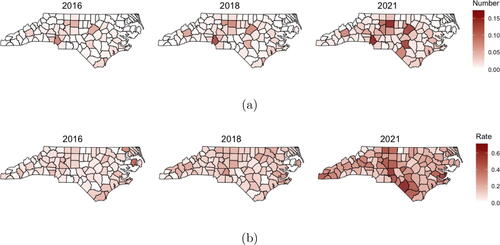
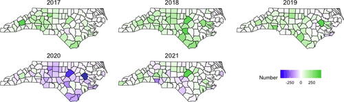
A goal of this analysis is to study how changes in the death rate relate to changes in the number of patients receiving buprenorphine. Figure 2 shows the county-level change in the number of patients with a buprenorphine prescription from the previous year so that green indicates an increase in the number of patients compared to the previous year, and purple indicates a decrease. Maps of the yearly number of buprenorphine patients and a line plot of the trend for each county are in the Supplementary Material. Prior to 2020, we observe a steady increase in the number of patients receiving buprenorphine in most counties across the state, with the state total increasing by 5231, 7478, and 5388 patients in 2017, 2018, and 2019, respectively. However, a decrease (4119 fewer patients across the state) occurred in 2020, which is likely due to challenges related to the COVID-19 pandemic. A moderate statewide increase of 1623 was observed in 2021, but for some counties, the decrease continued, and even for the counties that showed increases, the overall number of patients had not recovered to pre-2020 levels.

Fig. 2 County-level changes from previous year in the number of patients receiving buprenorphine.

While our goal is to study the relationship between changes in illicit opioid death rates and changes in the number of patients receiving buprenorphine, we include other variables in our model to account for socio-economic status of a county and also access to other forms of treatment that are distributed through OTPs (i.e., methadone). Counts of the number of certified OTPs were obtained by identifying all certified OTPs in North Carolina and their date of certification through the SAMSHA OTP directory (https://dpt2.samhsa.gov/treatment/) and then aggregating to the county-level. From 2016 to 2021, the total number of OTPs in the state increased from 42 to 72, with just 47 of the 100 counties having at least one OTP in 2021. We include the unemployment rate (number unemployed per 1000 total population) as a proxy of the socio-economic status of a county. On average, the unemployment rate was decreasing from 2016 to 2019, but drastically increased in 2020 before dropping again in 2021. Including unemployment in the model thus not only serves as a proxy to explain spatial variability related to socioeconomic status, but it also helps to capture the observed societal volatility in 2020 related to the COVID-19 pandemic. Maps of OTPs and unemployment rate are shown in the supplementary material.

2.2 Statistical Model

We develop a Bayesian hierarchical model to model the yearly count of illicit opioid overdose deaths for each county. The goal is to build a model that relates changes in the death rate to changes in the number of residents receiving buprenorphine prescriptions in order to quantify the impact that allocation of this resource has on overdose deaths.

To achieve this goal, we use a Poisson autoregressive model for the death counts (Agosto and Giudici 2020). More specifically, let Y_it be the number of deaths due to illicit opioid overdose in county $i=1,\dots ,n=100$ during year $t=1,\dots ,T=6$, where t = 1 corresponds to year 2016 and T = 6 to year 2021. We assume (1) $$Y_{it}|{\theta }_{it}\sim \text{Poisson}({\theta }_{it}),$$(1) where θ_it is the expected death count for county i in year t. The Poisson autoregressive model assumes the death rate in year t depends on the rate in year t – 1. More specifically, we assume a log-linear model of the form, where P_it is the population of county i in year t (in thousands), ${\mathit{X}}_{it}^{(1)}$ and ${\mathit{X}}_{it}^{(2)}$ are vectors of covariates, $\mathit{\alpha }$ and $\mathit{\beta }$ are vectors of regression coefficients, ${\varphi }_i^{(1)}$ and ${\varphi }_i^{(2)}$ are spatial random effects, and ${ϵ}_i\stackrel{\text{iid}}{\sim }N(0,{\sigma }^2)$. (2) $$\begin{array}{cc}\hspace{0.17em}\log \hspace{0.17em}\left(\frac{{\theta }_{it}}{P_{it}}\right)\hfill & ={\mathit{X}}_{it}^{(1)}\mathit{\alpha }+{\varphi }_i^{(1)}+{ϵ}_i, \text{ for }t=1\hfill \\ \hspace{0.17em}\log \hspace{0.17em}\left(\frac{{\theta }_{it}/P_{it}}{{\theta }_{i,t-1}/P_{i,t-1}}\right)\hfill & ={\mathit{X}}_{it}^{(2)}\mathit{\beta }+{\varphi }_i^{(2)}, \text{ for }t\ge 2\hfill \end{array}$$(2)

Note that the equations in (2) are equivalent to (3) $$\begin{array}{cc}\hspace{0.17em}\log \hspace{0.17em}({\theta }_{it})\hfill & =\hspace{0.17em}\log \hspace{0.17em}(P_{it})+{\mathit{X}}_{it}^{(1)}\mathit{\alpha }+{\varphi }_i^{(1)}+{ϵ}_i, \text{ for }t=1\hfill \\ \hspace{0.17em}\log \hspace{0.17em}({\theta }_{it})\hfill & =\hspace{0.17em}\log \hspace{0.17em}(P_{it})+\hspace{0.17em}\log \hspace{0.17em}({\theta }_{i,t-1})-\hspace{0.17em}\log \hspace{0.17em}(P_{i,t-1})+{\mathit{X}}_{it}^{(2)}\mathit{\beta }+{\varphi }_i^{(2)},\hfill \\ \hfill & \mathrm{\hspace{1em}}\mathrm{\hspace{1em}}\text{ for }t=2,\dots ,T.\hfill \end{array}$$(3)

We are primarily interested in changes in the death rate which will be quantified through the model for $t=2,\dots ,T$. However, we must specify a model for t = 1 to establish a baseline rate. The covariates used in the model for t = 1 are ${\mathbf{X}}_{i1}^{(1)}=(1,{\mathrm{T}}_{i1},{\mathrm{U}}_{i1},{\mathrm{B}}_{i1}),$ where ${\mathrm{T}}_{it}$ refers to the number of opioid treatment programs in county i in year t, ${\mathrm{U}}_{it}$ refers to the unemployment rate, and ${\mathrm{B}}_{it}$ refers to the number of patients receiving buprenorphine prescriptions. The spatial random effect ${\varphi }_i^{(1)}$ is assumed to follow an intrinsic conditional autoregressive (ICAR) model. That is, for each location $i=1,\dots ,n$ (4) $${\varphi }_i^{(1)}|{\varphi }_{j\ne i}^{(1)}\sim N\left(\frac{1}{m_i}\sum _{j\sim i}{\varphi }_j^{(1)},\frac{{\tau }_1^2}{m_i}\right),$$(4) where $j\sim i$ indicates all counties j that are neighbors (share a border) with county i, and m_i denotes the number of neighbors for county i. Note that the ICAR model is an improper density since the resulting precision matrix of the vector ${\mathit{\varphi }}^{(1)}=({\varphi }_1^{(1)},\dots {\varphi }_{100}^{(1)})$ is less than full rank, but it can be used as a prior distribution on the random effects and yields a proper posterior distribution provided the centering constraint, $\sum _i{\varphi }_i^{(1)}=0$, is enforced (Banerjee, Carlin, and Gelfand 2003). We include an additional independent, identically distributed error term in the baseline model in order to capture additional unexplained heterogeneity in the baseline death rate. This extra variability will propagate through the rate for years $t=2,\dots ,T$ given the autoregressive structure of the model.

Recall, a primary goal is to quantify how changes in the number of residents receiving buprenorphine relates to the change in death rate. Thus, a focus of our inference is to estimate $\mathit{\beta }$ in the model for years $t=2,\dots ,T$ for which the design matrix is of the form ${\mathbf{X}}_{it}^{(2)}=(1,t,{\mathrm{T}}_{it},{\mathrm{U}}_{it},\Delta {\mathrm{B}}_{it}),$ where ${\mathrm{T}}_{it}$ and ${\mathrm{U}}_{it}$ are as defined above and $\Delta {\mathrm{B}}_{it}={\mathrm{B}}_{it}-{\mathrm{B}}_{i,t-1}$ is the difference in the number of patients receiving buprenorphine prescriptions in year t compared to year t – 1. We include a spatial random effect ${\varphi }_i^{(2)}$ to account for additional spatial heterogeneity that is not accounted for with the other covariates. We assume this quantity has an ICAR model analogous to the model for ${\varphi }_i^{(1)}$ but with conditional variance parameter ${\tau }_2^2$. This random effect is static across time because we believe the spatial dependence and residual spatial heterogeneity should be constant over this short time period after accounting for the other variables in the model.

Since we are using a Bayesian framework, we need to specify prior distributions for all remaining parameters in the model. We assume all regression coefficients in $\mathit{\alpha }$ and $\mathit{\beta }$ have diffuse zero-mean normal prior distributions with variance 1000. The variance parameters ${\sigma }^2,{\tau }_1^2$, and ${\tau }_2^2$ are assigned inverse gamma prior distributions with shape and scale parameters of 0.1. Let $[Z]$ denote the probability distribution function of a random variable Z and $[W|Z]$ the conditional distribution of a random variable W conditional on Z. Using this bracket notation, the posterior distribution for this model is of the form (5) $$\begin{array}{c}\left[\mathit{\alpha },\mathit{\beta },{\mathit{\varphi }}^{(1)},{\mathit{\varphi }}^{(2)},\mathbf{ϵ},{\sigma }^2,{\tau }_1^2,{\tau }_2^2|\mathit{Y}\right]\\ \hspace{1em}\propto \left[{\mathit{Y}}_1\right|\mathit{\alpha },{\mathit{\varphi }}^{(1)},\mathbf{ϵ}\left]\prod _{t=2}^T\right[{\mathit{Y}}_t|\mathit{\beta },{\mathit{\varphi }}^{(2)}]\\ \mathrm{\hspace{1em}}\mathrm{\hspace{1em}}\times \left[{\mathit{\varphi }}^{(1)}\right|{\tau }_1^2\left]\right[{\mathit{\varphi }}^{(2)}\left|{\tau }_2^2\right]\left[\mathbf{ϵ}\right|{\sigma }_1^2\left]\right[\mathit{\alpha },\mathit{\beta },{\sigma }^2,{\tau }_1^2,{\tau }_2^2].\end{array}$$(5)

The posterior distribution can be simulated using a Metropolis-within-Gibbs Markov chain Monte Carlo (MCMC) algorithm. We used the R package NIMBLE to implement an MCMC algorithm to simulate from the posterior distribution (de Valpine et al. 2017, 2022). We standardize all covariates in order to assist with mixing in the MCMC algorithm.

2.3 Optimizing Resource Allocation

In Section 2.2, we built a model to relate the change in the amount of an opioid-related resource available to the change in the death rate due to illicit opioid overdose. A natural follow-up question is: If additional resources for the state become available, how should these be distributed across the counties? In this article, we focus on increasing the number of patients with a buprenorphine prescription. Given the buprenorphine waiver certificate requirements and the restrictions on who can prescribe buprenorphine and how many patients they can prescribe to, estimating where and how many more prescriptions would be most beneficial can help identify counties that should be targeted for increasing the number and capacity of waivers. We propose a constrained nonlinear optimization approach where bounds on the statewide and county-specific increases are assumed, and the objective function to minimize is based on the posterior predictive distribution of future expected illicit opioid overdose deaths, obtained using the model from Section 2.2.

2.3.1 Single-Year Optimization

We start by considering two objective functions as our criteria to minimize. First, we consider the estimated statewide total expected number of deaths in the next year, given by ${\widehat{\Theta }}_{T+1}={\sum }_{i=1}^{100}{\widehat{\theta }}_{i,T+1}$. Since ${\widehat{\Theta }}_{T+1}$ has the potential to be influenced by the most populous counties, we also consider the estimated state average rate per 1000, ${\widehat{R}}_{T+1}=\frac{1}{100}{\sum }_{i=1}^{100}{\widehat{\theta }}_{i,T+1}/P_{i,T+1}$. To make the dependence on the change in buprenorphine more explicit, we modify the notation and define ${\gamma }_{i,T+1}\equiv \hspace{0.17em}\log \hspace{0.17em}(P_{i,T+1})-\hspace{0.17em}\log \hspace{0.17em}(P_{i,T})+{\overline{\mathit{X}}}_{i,T+1}^{(2)}\overline{\mathit{\beta }}+{\varphi }_i^{(2)}$, where ${\overline{\mathit{X}}}_{i,T+1}^{(2)}$ and $\overline{\mathit{\beta }}$ are subsets of the vectors, excluding the components that correspond to $\Delta {\mathrm{B}}_{i,T+1}$. Then, (2) becomes $$\hspace{0.17em}\log \hspace{0.17em}({\theta }_{i,T+1})=\hspace{0.17em}\log \hspace{0.17em}({\theta }_{i,T})+{\gamma }_{i,T+1}+{\beta }_B\Delta {\mathrm{B}}_{i,T+1},$$where β_B is the element of $\mathit{\beta }$ that corresponds to the regression coefficient for the change in buprenorphine $\Delta \mathrm{B}$. Using this notation, the estimated state total expected number of deaths in year T + 1 is (6) $$\begin{array}{c}{\widehat{\Theta }}_{T+1}=\sum _{i=1}^{100}{\widehat{\theta }}_{i,T+1}=\sum _{i=1}^{100}{\widehat{\theta }}_{i,T}\hspace{0.17em}\exp \hspace{0.17em}\left({\widehat{\gamma }}_{i,T+1}+{\widehat{\beta }}_B\Delta {\mathrm{B}}_{i,T+1}\right)\\ =\sum _{i=1}^{100}{c}_i\hspace{0.17em}\exp \hspace{0.17em}\left({\widehat{\beta }}_B\Delta {\mathrm{B}}_{i,T+1}\right),\end{array}$$(6) and the estimated average death rate is (7) $$\begin{array}{c}{\widehat{R}}_{T+1}=\frac{1}{100}\sum _{i=1}^{100}{\widehat{\theta }}_{i,T+1}/P_{i,T+1}\\ =\frac{1}{100}\sum _{i=1}^{100}{c}_i\hspace{0.17em}\exp \hspace{0.17em}\left({\widehat{\beta }}_B\Delta {\mathrm{B}}_{i,T+1}\right)/P_{i,T+1},\end{array}$$(7) where $c_i={\widehat{\theta }}_{i,T}\hspace{0.17em}\exp \hspace{0.17em}({\widehat{\gamma }}_{i,T+1}),$ ${\widehat{\gamma }}_{i,T+1}=\hspace{0.17em}\log \hspace{0.17em}(P_{i,T+1})-\hspace{0.17em}\log \hspace{0.17em}(P_{i,T})+{\overline{\mathit{X}}}_{i,T+1}^{(2)}\widehat{\overline{\mathit{\beta }}}+{\widehat{\varphi }}_i^{(2)}$, and ${\widehat{\theta }}_{i,T},\widehat{\overline{\mathit{\beta }}},{\widehat{\varphi }}_i^{(2)},{\widehat{\beta }}_B$ are the estimated posterior means computed using the MCMC output from fitting the model to the observed data. We note that the objective functions depend on the population (in thousands), $P_{i,T+1}$, unemployment rate ${\mathrm{U}}_{i,T+1}$, and number of OTPs ${\mathrm{T}}_{i,T+1}$ in year T + 1. In practice, values of the population and explanatory variables for a future year are unknown. For the purpose of forecasting future death rate as a function of $\Delta \mathrm{B}$, we assume these other values do not change from t = T to $t=T+1$ (e.g., $P_{i,T+1}=P_{i,T}$). Alternatively, one could model these variables within the Bayesian hierarchical model and then forecast the values in year T + 1 by simulating from the posterior predictive distribution.

To identify the “optimal” resource allocation scheme under each objective function, we view ${\widehat{\Theta }}_{T+1}$ and ${\widehat{R}}_{T+1}$ as functions of the n = 100 unknown variables $\Delta {\mathrm{B}}_{1,T+1},\dots ,\Delta {\mathrm{B}}_{100,T+1}$, and we seek to find the values of $\Delta {\mathrm{B}}_{1,T+1},\dots ,\Delta {\mathrm{B}}_{100,T+1}$ that minimize these objective functions, subject to constraints on the state’s total increase and bounds on each county’s increase. More specifically, we force $\sum _i\Delta {\mathrm{B}}_{i,T+1}=a$, and for each $i=1,\dots ,100$, we restrict $\mathcal{l}\le \Delta {\mathrm{B}}_{i,T+1}\le u$, where a, $\mathcal{l}$, and u are pre-specified values.

2.3.2 Multi-Year Optimization

Minimizing ${\widehat{\Theta }}_{T+1}$ and ${\widehat{R}}_{T+1}$ provides optimal allocation plans for the next year. We can extend our question to provide the allocation plan for a multi-year strategy. Suppose we want to provide an allocation scheme for the next three years, $t=T+1,T+2,T+3$, which for our data, corresponds to 2022, 2023, and 2024. We can instead consider the statewide total deaths ${\Theta }_{T+1:T+3}$ and average rate $R_{T+1:T+3}$ aggregated over the three year period and view these objective functions as functions of the 300 unknown changes in the number of patients receiving buprenorphine in each county during each year. More formally, the recursive definition of ${\theta }_{i,t}$ allows us to write (8) $$\begin{array}{cc}\hfill & {\Theta }_{T+1:T+3}\equiv \sum _{i=1}^{100}\sum _{\mathcal{l}=1}^3{\theta }_{i,T+\mathcal{l}}=\sum _{i=1}^{100}\sum _{\mathcal{l}=1}^3{\theta }_{i,T+\mathcal{l}-1}{e}^{{\gamma }_{T+\mathcal{l}}}{e}^{{\beta }_B\Delta {\mathrm{B}}_{i,T+\mathcal{l}}}\hfill \\ \hfill & =\sum _{i=1}^{100}({\theta }_{i,T}{e}^{{\gamma }_{T+1}}{e}^{{\beta }_B\Delta {\mathrm{B}}_{i,T+1}}+{\theta }_{i,T+1}{e}^{{\gamma }_{T+2}}{e}^{{\beta }_B\Delta {\mathrm{B}}_{i,T+2}}\hfill \\ \hfill & \mathrm{\hspace{1em}}\mathrm{\hspace{1em}}+{\theta }_{i,T+2}{e}^{{\gamma }_{T+3}}{e}^{{\beta }_B\Delta {\mathrm{B}}_{i,T+3}})\hfill \\ \hfill & =\sum _{i=1}^{100}{\theta }_{i,T}{e}^{{\gamma }_{T+1}}{e}^{{\beta }_B\Delta {\mathrm{B}}_{i,T+1}}(1+e^{{\gamma }_{T+2}}{e}^{{\beta }_B(\Delta {\mathrm{B}}_{i,T+2})}\hfill \\ \hfill & \mathrm{\hspace{1em}}\mathrm{\hspace{1em}}+e^{{\gamma }_{T+2}+{\gamma }_{T+3}}{e}^{{\beta }_B(\Delta {\mathrm{B}}_{i,T+2}+\Delta {\mathrm{B}}_{i,T+3})}),\hfill \end{array}$$(8) and (9) $$\begin{array}{cc}\hfill & R_{T+1:T+3}\equiv \frac{1}{300}\sum _{i=1}^{100}\sum _{\mathcal{l}=1}^3{\theta }_{i,T+\mathcal{l}}/P_{i,T+\mathcal{l}}\hfill \\ \hfill & =\frac{1}{300}\sum _{i=1}^{100}{\theta }_{i,T}{e}^{{\gamma }_{T+1}}{e}^{{\beta }_B\Delta {\mathrm{B}}_{i,T+1}}(\frac{1}{P_{i,T+1}}+\frac{e^{{\gamma }_{T+2}}{e}^{{\beta }_B(\Delta {\mathrm{B}}_{i,T+2})}}{P_{i,T+2}}\hfill \\ \hfill & \mathrm{\hspace{1em}}\mathrm{\hspace{1em}}+\frac{e^{{\gamma }_{T+2}+{\gamma }_{T+3}}{e}^{{\beta }_B(\Delta {\mathrm{B}}_{i,T+2}+\Delta {\mathrm{B}}_{i,T+3})}}{P_{i,T+3}}).\hfill \end{array}$$(9)

As in Section 2.3.1, we assume the population and remaining covariates remain unchanged so that $P_{i,T+\mathcal{l}}=P_{i,T}$ and ${\overline{X}}_{i,T+\mathcal{l}}^{(2)}={\overline{X}}_{i,T}^{(2)}$ for $\mathcal{l}=1,2,3$. We consider the estimated total count and average rate, ${\widehat{\Theta }}_{T+1:T+3}$ and ${\widehat{R}}_{T+1:T+3}$, which are computed by replacing quantities in the definition with the estimated posterior means resulting from the model fit to the observed data. Then, we use constrained nonlinear optimization to find the values $\{\Delta {\mathrm{B}}_{i,T+\mathcal{l}}:i=1,\dots ,100;\mathcal{l}=1,2,3\}$ that minimize ${\widehat{\Theta }}_{T+1:T+3}$ and ${\widehat{R}}_{T+1:T+3}$ subject to the constraints ${\sum }_{i=1}^{100}{\sum }_{\mathcal{l}=1}^3\Delta {\mathrm{B}}_{i,T+\mathcal{l}}=a_3$ and ${\mathcal{l}}_3\le \Delta {\mathrm{B}}_{i,T+\mathcal{l}}\le u_3$ for each $i=1,\dots ,100$ and $\mathcal{l}=1,2,3$.

3 Results

3.1 Model Results

We ran two chains of the MCMC algorithm for 1,500,000 iterations each with burn-ins of 1,000,000 iterations. We thinned the output by keeping every 50th iteration. We confirmed convergence by visually inspecting trace plots and by computing the Gelman-Rubin statistic. Posterior predictive p-values based on the mean and standard deviation were 0.5081 and 0.5704, respectively, so there was no evidence of lack of model fit.

In this section, we provide results for the t > 1 model as that was the target of our inference. Estimates of the regression coefficients for the baseline model are provided in the supplementary material. Table 1 provides estimates and 95% credible intervals for the regression coefficients $\mathit{\beta }$ from the autoregressive model. Recall that the covariates in the model were standardized to be mean zero with standard deviation one, and also recall from (2) $$\frac{{\theta }_{it}}{P_{it}}=\frac{{\theta }_{i,t-1}}{P_{i,t-1}}\times e^{{\mathbf{X}}_{it}^{(2)}\mathit{\beta }+{\varphi }_i^{(2)}}.$$

Table 1 Posterior means and 95% credible intervals for regression coefficients in the t > 1 model.

Variable	Estimate	95% C.I.
Intercept	0.3532	(0.2689, 0.4488)
Time, t	–0.0343	(–0.0557, –0.0134)
Opioid treatment programs	–0.0203	(–0.0400, –0.0011)
Unemployment rate	0.0709	(0.0455, 0.0987)
ΔBuprenorphine	–0.0211	(–0.0429, 0.0003)

Thus, the model estimates, on average, that the rate multiplies by $e^{0.3532}=1.4236$ each year, but the slight negative time trend implies the multiplicative change in the rate is getting smaller over time (although still positive throughout this study). We observe a positive association with unemployment, with an estimated rate ratio of $e^{0.0709}=1.0734$ per standard deviation increase in unemployment, with 95% credible interval of (1.0466, 1.1037). We estimate a negative association with the change in buprenorphine patients, with the model estimating a rate ratio of $e^{-0.0211}=0.9791$ per standard deviation increase in ΔBuprenorphine, with credible interval (0.9580, 1.0003). Although this credible interval contains 1.0, we note that 97.18% of the posterior distribution of $e^{{\beta }_B}$ was less than one. Supplemental Figure 7 shows a map of the estimated spatial random effect, ${\varphi }_i^{(2)}$ as well as its standard error. This captures spatial heterogeneity in the change of the death rate that is unmeasured by the covariates.

We simulated from the posterior predictive distribution to predict the county-level number of illicit opioid overdose deaths for each county during the time period under study and also for the next three years. For the forecasts of the next three years, we assumed there were no changes in population size, buprenorphine patients, OTPs, or unemployment rate, as compared to the values in t = T. This assumption will serve as our baseline model for comparison in the next section. Let ${\tilde{y}}_{it}$ denote the predicted counts under our model and these assumptions for county $i=1,\dots ,100$ in year $t=1,\dots ,T+3$. 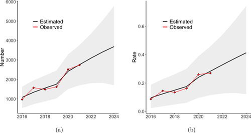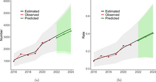We aggregated over the state to predict the yearly state total number of deaths, $\sum _i{\tilde{y}}_{it}$, and also the yearly state average rate of deaths, $\frac{1}{100}\sum _i{\tilde{y}}_{it}/P_{it}.$ Figure 3 shows the posterior mean of the predicted statewide values and 95% credible intervals for the predictions, as well as the observed statewide values. From this plot, we can see our model captures the statewide trend over this time period. Under the assumption of no change in the covariates, our model predicts the state will observe 3,092, 3,405, and 3,686 illicit opioid overdose deaths in 2022, 2023, and 2024, respectively, which corresponds to statewide average illicit opioid overdose death rates of 0.328, 0.371, and 0.413 per 1000. 95% credible bounds for these predictions are shown in the figure.

Fig. 3 (a) Yearly estimated state total number with 95% credible intervals. (b) Yearly estimated state rate with 95% credible intervals. The black line is the mean of the posterior predictive distribution from the model fit to the observed data and then forecasted assuming no change in the covariates. The red points are the observed values.

3.2 Resource Allocation Result

Next, we continue to assume the population, number of OTPs, and unemployment rate remain unchanged for each county after year T. However, the number of patients with a prescription for buprenorphine is unknown after year T, and the state expected total illicit opioid death count, ${\widehat{\Theta }}_{T+1}$, and average rate, ${\widehat{R}}_{T+1}$, are functions of this change in buprenorphine, $\Delta {\mathrm{B}}_{i,T+1}$. The estimated quantities in (6) and (7) are posterior means from the model fit in Section 3.1. Recall our goal is to find the values for the change in buprenorphine, $\Delta {\mathrm{B}}_{1,T+1},\dots ,\Delta {\mathrm{B}}_{n,T+1}$ that minimize ${\widehat{\Theta }}_{T+1}$ and ${\widehat{R}}_{T+1}$, subject to constraints.

We used the nloptr package in R to perform nonlinear constrained optimization using the Augmented Lagrangian method (Johnson 2021; Bhadani 2021). For illustration, we assume that the statewide total increase in the number of buprenorphine patients in year T + 1 is 6743, which is equal to the average statewide total difference observed in 2017, 2018, and 2019. We assume the change in the number of buprenorphine patients in each county is bounded below by 0 and bounded above by 464, which was the largest yearly increase observed by any county during the previous six-year period. We performed the optimization twice—once using the statewide total expected count, ${\widehat{\Theta }}_{T+1}$, as the objective function, and once using the average rate, ${\widehat{R}}_{T+1}$.

Table 2 shows the 10 counties with the largest recommended increases of buprenorphine patients under the two optimal allocation strategies identified by the objective functions. Figure 4 shows maps of the optimal increase for each county under the two scenarios. Observe that when the goal was to minimize the state total number of illicit opioid overdose deaths, the optimal allocation scheme largely prioritizes more populous counties that had the highest absolute observed death counts (refer to Figure 1(a)). When the estimated state average rate of illicit opioid overdose deaths was used as the objective function, the resulting allocation scheme is quite different and recommends larger increases in counties where the current number of patients receiving buprenorphine is low relative to the high death rate shown in Figure 1(b). We also note that optimizing based on minimizing the state rate resulted in more dispersion across the counties compared to the scheme based on the statewide total. More specifically, when minimizing the statewide total number of illicit opioid overdose deaths, the median amount of increase suggested was 0 with 10 counties receiving the upper bound on the increase (464 patients) and 77 counties suggested to have zero increase; whereas when the state average rate was minimized, the median amount of increase was 66 with 3 counties receiving the upper bound and 19 counties suggested to have zero. Supplemental Tables 2 and 3 contain the optimal amount of increase for each county under both objective functions.

Fig. 4 Maps of the results for the resource allocation optimization approach. The left map shows the optimal increase in buprenorphine patients to minimize the expected state total, ${\widehat{\Theta }}_{T+1}$. The right map shows the optimal increase required to minimize the rate, ${\widehat{R}}_{T+1}$. The seven most populous counties are indicated by triangles, with the size of the triangle proportional to the population size of that county.

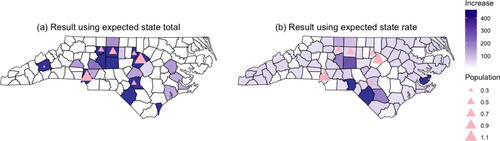
Table 2 Results for expanding buprenorphine using total expected death.

Minimize ${\widehat{\Theta }}_{T+1}$		Minimize ${\widehat{R}}_{T+1}$
County	Increase	County	Increase
Buncombe	464	Pamlico	464
Cumberland	464	Robeson	464
Davidson	464	Richmond	460
Durham	464	Randolph	349
Forsyth	464	Davidson	243
Guilford	464	Bladen	239
New Hanover	464	Stokes	151
Mecklenburg	464	Lee	118
Randolph	464	Rockingham	109
Robeson	464	Cumberland	94

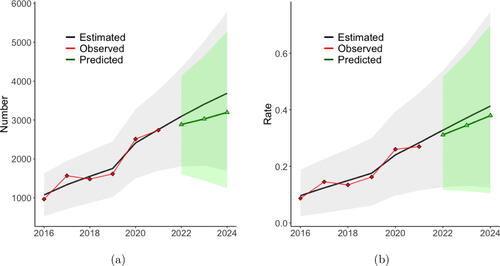
As in Section 2.2, we simulated from the posterior predictive distribution to predict the county-level number of illicit overdose deaths for each county for the next three years. However, instead of assuming all covariates remain unchanged, we assume $\Delta {\mathrm{B}}_{i,T+1}$ is the value identified by the optimization and then remains constant in years T + 2 and T + 3. Figure 5(a) shows the predicted state total number of deaths when the optimal allocation scheme that minimizes the state total expected count is implemented. Under this scenario, our model estimates there will be 2930 deaths in 2022, which is a decrease of 162 (5.23%) from the base case value of 3092. We note that the credible intervals for the predicted count are wide with substantial overlap. However, the Bayesian approach taken here allows us to estimate the probability of a decrease in the outcome under the two schemes considered. The posterior probability that the 2024 count of illicit opioid overdose deaths is decreased under the optimal allocation scheme is 0.9297, which is quite high. Figure 5(b) shows the predicted state average death rate when the allocation scheme that minimizes the state average rate is implemented. In this case, our model estimates the state average rate in 2022 will be 0.320, which is a reduction of 0.0077 (2.35%) in the average rate per 1000 compared to the baseline. The posterior probability that the 2024 average rate of illicit opioid overdose deaths is decreased is 0.7364.

Fig. 5 (a) Yearly estimated state total number with 95% credible intervals. (b) Yearly estimated state rate with 95% credible intervals. The black line is the mean of the posterior predictive distribution from the model fit to the observed data and then forecasted assuming no change in the covariates. The red points are the observed values. The green points and line are the posterior means of the forecasted totals assuming the change in buprenorphine value in year T + 1 is as identified by the optimization procedure.

We note that the credible intervals for the predicted count and rate are wide with substantial overlap. However, the Bayesian approach taken here allows us to estimate the probability of a decrease in the outcome, and the estimated probability of 0.9297 for the count and 0.7364 for the rate are

Note that in Figure 5, the trends remain relatively constant through 2024 because the forecast is done by implementing the allocation scheme in 2022 and then assuming no additional changes in 2023 or 2024. Next, we repeat the optimization using the multi-year strategy outlined in Section 2.3.2 where we seek to minimize ${\widehat{\Theta }}_{T+1:T+3}$ and ${\widehat{R}}_{T+1:T+3}$ as defined in (8) and (9), respectively. We assume the state total increase in buprenorphine over the 3-year period is $3(6743)=20,229$, and each county’s yearly increase is bounded between 0 and 464, as before. Figure 6(a) shows the predicted state total number of illicit opioid overdose deaths assuming we implement the allocation scheme that optimally minimizes ${\widehat{\Theta }}_{T+1:T+3}$. The predicted number of deaths in the three years are 9104, which is a total decrease of 1078 (10.59%) compared to baseline. The posterior probability that the 2024 count of illicit opioid overdose deaths is decreased is 0.9773. Figure 6(b) shows the predicted state average rate of illicit opioid overdose deaths assuming we implement the allocation scheme that minimizes ${\widehat{R}}_{T+1:T+3}$. The predicted average rate over the 3-year period is 0.3450, which is a 0.0256 reduction (6.91%) from the baseline average rate. The posterior probability that the 2024 average rate of illicit opioid overdose deaths is decreased is 0.9278. Maps of the suggested increase in buprenorphine patients under this multi-year approach are shown in Supplemental Figure 8. The map shows that it is optimal to allocate most of the 20,229 new buprenorphine prescriptions during the first year.

Fig. 6 (a) Yearly estimated state total number with 95% credible intervals. (b) Yearly estimated state rate with 95% credible intervals. The black line is the mean of the posterior predictive distribution from the model fit to the observed data and then forecasted assuming no change in the covariates. The red points are the observed values. The green points and line are the posterior means of the forecasted totals assuming the changes in buprenorphine in year 2022, 2023, and 2024 as identified by the multi-year optimization procedure.

4 Discussion

In this article, we implemented a statistical approach to the problem of geographical resource allocation. First, we develop a Bayesian spatio-temporal Poisson autoregressive model to quantify how changes in the resource of interest relate to changes in the outcome. Then, we use the posterior predictive distribution from our model to define an objective function to be minimized. The proposed “optimal” resource allocation scheme is the set of location-specific changes in the resource that minimize the objective function under a set of constraints on the available resources. Lastly, we simulate from the posterior predictive distribution assuming the optimal allocation scheme is implemented in order to quantify the effect of the additional resources.

Existing approaches to resource allocation are dominated by mechanistic models which rely on either assumptions regarding model inputs or data on individuals or sub-populations in order to estimate the inputs. Those approaches are not well suited when only aggregate data is available. Our proposed framework using a Bayesian autoregressive spatio-temporal model to forecast an outcome of interest instead of a mechanistic model circumvents this shortcoming and also seamlessly propagates uncertainty through to the predictions.

We illustrated our approach using yearly, county-level data from North Carolina to identify the optimal increases in the number of patients receiving buprenorphine in order to minimize the expected statewide total number and average rate of illicit opioid overdose deaths. This question is especially timely given recent changes to the requirements needed to receive a waiver to prescribe buprenorphine (U.S. Department of Health and Human Services 2021). Our model estimates a negative relationship between increases in the number of buprenorphine prescriptions and the multiplicative change in illicit opioid overdose death rate. Our resource allocation strategy provides recommended increases for each county. The results of the resource allocation depend on the objective function to be minimized and the constraints enforced. When the statewide expected total number of deaths was the objective function, the approach prioritized more populous counties than when the statewide average rate was minimized. We implemented our strategy under a set of constraints that were approximately equal to historical changes, but ideally these would be informed by the public health infrastructure. Also, in our application we assumed the same lower and upper bounds for all counties, but in practice these can differ based on the individual counties’ capacities. Our model allowed us to not only identify the “optimal” resource allocation scheme, but also to estimate the effect of the allocation compared to the baseline.

There are several shortcomings to the current approach. First, we assumed the population size and covariates (excluding the covariate of interest) remained constant when predicting for future years. Instead, we could expand our Bayesian model to include process-level models for these quantities so that uncertainty regarding those values is accounted for. Relatedly, in practice it is likely the case that more than one resource is being implemented or expanded at the same time. In the future, we will expand this work to consider multiple interacting resources simultaneously. More specifically, we will consider the multivariate setting where we will optimize allocation plans over multiple resources. This will allow us to identify synergistic effects and explore potential tradeoffs among different resources. Second, future work will include a more in-depth study as to the choices of objective function and constraints and the impact that those have on the results. One direction is to use a bivariate loss function that addresses cost considerations. By incorporating costs into the allocation decision-making process, we can assess resource utilization in both reducing opioid overdose mortality and controlling cost, which aligns with our goal to make efficient use of limited resources. Lastly, we will work to adapt our approach so that instead of optimizing under a set of constraints on the resources, we will identify an allocation strategy that will help reach a targeted reduction in the outcome. For example, the NCDHHS OSUAP 3.0 states a goal of reducing all drug overdose deaths by 20% from expected by 2024 (North Carolina Department of Health and Human Services 2021). The 3-year optimization scheme in Section 2.3 based on minimizing the statewide total under a given set of constraints predicted a reduction in illicit opioid overdose deaths of 10% from expected. A possible question of interest then is what geographical allocation achieves the targeted reduction while using the fewest amount of resources possible?

The geographical allocation of resources for public health outcomes is a challenging question but is of the utmost importance. Historically, approaches to this question have relied on mechanistic models, which are not necessarily available or practical for all public health outcomes. In recent years, there has been an increase in the amount of surveillance data that is available in order to track trends in public health. In this article, we have developed and proposed a data-driven approach to resource allocation. This framework uses observed data to estimate trends and is broadly applicable to many outcomes in public health. This work can help guide future policy responses to public health crises and also serve as a springboard to further statistical development in this area.

Supplementary Materials

The supplementary materials contain additional figures and results from the analysis. All data and code needed to implement both the MCMC and optimization algorithm are also available.

Acknowledgments

The authors would like to acknowledge the North Carolina Department of Health and Human Services for making the data used in this analysis publicly available. In particular, we thank Scott Proescholdbell and Mary Beth Cox for help accessing the data and for insightful conversations during the research process.

Additional information

Funding

Research reported in this publication was supported by the National Institute On Drug Abuse of the National Institutes of Health under Award Number R01DA052214. The content is solely the responsibility of the authors and does not necessarily represent the official views of the National Institutes of Health.

References

- Agosto, A., and Giudici, P. (2020), “A Poisson Autoregressive Model to Understand COVID-19 Contagion Dynamics,” Risks, 8, 77. DOI: 10.3390/risks8030077.
- Ahmad, F., Cisewski, J., Rossen, L., and Sutton, P. (2022), “Provisional Drug Overdose Death Counts,” available at https://www.cdc.gov/nchs/nvss/vsrr/drug-overdose-data.htm.
- Antonelli, J., and Beck, B. (2020), “Heterogeneous Causal Effects of Neighborhood Policing in New York City with Staggered Adoption of the Policy,” arXiv preprint arXiv:2006.07681.
- Banerjee, S., Carlin, B. P., and Gelfand, A. E. (2003), Hierarchical Modeling and Analysis for Spatial Data, Boca Raton, FL: Chapman and Hall/CRC.
- Barnett, P. G., Zaric, G. S., and Brandeau, M. L. (2001), “The Cost–Effectiveness of Buprenorphine Maintenance Therapy for Opiate Addiction in the United States,” Addiction, 96, 1267–1278. DOI: 10.1046/j.1360-0443.2001.96912676.x.
- Battista, N. A., Pearcy, L. B., and Strickland, W. C. (2019), “Modeling the Prescription Opioid Epidemic,” Bulletin of Mathematical Biology, 81, 2258–2289. DOI: 10.1007/s11538-019-00605-0.
- Bernard, C. L., Owens, D. K., Goldhaber-Fiebert, J. D., and Brandeau, M. L. (2017), “Estimation of the Cost-Effectiveness of HIV Prevention Portfolios for People Who Inject Drugs in the United States: A Model-based Analysis,” PloS Medicine, 14, e1002312. DOI: 10.1371/journal.pmed.1002312.
- Bhadani, R. (2021), “Nonlinear Optimization in R Using nlopt,” arXiv preprint arXiv:2101.02912 .
- Castillo-Carniglia, A., Ponicki, W., Gaidus, A., Gruenewald, P., Marshall, B. D., Fink, D. S., Martins, S. S., Rivera-Aguirre, A., Wintemute, G. J., and Cerdá, M. (2019), “Prescription Drug Monitoring Programs and Opioid Overdoses: Exploring Sources of Heterogeneity,” Epidemiology (Cambridge, Mass.), 30, 212. DOI: 10.1097/EDE.0000000000000950.
- Cerdá, M., Jalali, M. S., Hamilton, A. D., DiGennaro, C., Hyder, A., Santaella-Tenorio, J., Kaur, N., Wang, C., and Keyes, K. M. (2022), “A Systematic Review of Simulation Models to Track and Address the Opioid Crisis,” Epidemiologic Reviews, 43, 147–165. DOI: 10.1093/epirev/mxab013.
- Chen, Q., Larochelle, M. R., Weaver, D. T., Lietz, A. P., Mueller, P. P., Mercaldo, S., Wakeman, S. E., Freedberg, K. A., Raphel, T. J., Knudsen, A. B., Pandharipande, P. V., and Chhatwal, J. (2019), “Prevention of Prescription Opioid Misuse and Projected Overdose Deaths in the United States,” p. 12.
- Ciccarone, D. (2019), “The Triple Wave Epidemic: Supply and Demand Drivers of the US Opioid Overdose Crisis,” International Journal of Drug Policy, 71, 183–188. DOI: 10.1016/j.drugpo.2019.01.010.
- de Valpine, P., Paciorek, C., Turek, D., Michaud, N., Anderson-Bergman, C., Obermeyer, F., Wehrhahn Cortes, C., Rodrìguez, A., Temple Lang, D., and Paganin, S. (2022), NIMBLE: MCMC, Particle Filtering, and Programmable Hierarchical Modeling. R package version 0.12.2. Available at https://cran.r-project.org/package=nimble
- de Valpine, P., Turek, D., Paciorek, C., Anderson-Bergman, C., Temple Lang, D., and Bodik, R. (2017), “Programming with Models: Writing Statistical Algorithms for General Model Structures with NIMBLE,” Journal of Computational and Graphical Statistics, 26, 403–413. DOI: 10.1080/10618600.2016.1172487.
- Delgado, M. S., and Florax, R. J. (2015), “Difference-in-Differences Techniques for Spatial Data: Local Autocorrelation and Spatial Interaction,” Economics Letters, 137, 123–126. DOI: 10.1016/j.econlet.2015.10.035.
- Guan, Q., Reich, B. J., and Laber, E. B. (2022), “A Spatiotemporal Recommendation Engine for Malaria Control,” Biostatistics, 23, 1023–1038. DOI: 10.1093/biostatistics/kxab010.
- Hedegaard, H., Miniño, A., Spencer, M. R., and Warner, M. (2022), “Drug Overdose Deaths in the United States, 1999–2020,” NCHS Data Brief (428).
- Irvine, M. A., Kuo, M., Buxton, J. A., Balshaw, R., Otterstatter, M., Macdougall, L., Milloy, M., Bharmal, A., Henry, B., Tyndall, M., Coombs, D., and Gilbert, M. (2019), “Modelling the Combined Impact of Interventions in Averting Deaths During a Synthetic-Opioid Overdose Epidemic,” Addiction, 114, 1602–1613. DOI: 10.1111/add.14664.
- Johnson, S. G. (2021), “The nlopt Nonlinear-Optimization Package,” available at https://nlopt.readthedocs.io/en/latest/.
- Kedziora, D. J., Stuart, R. M., Pearson, J., Latypov, A., Dierst-Davies, R., Duda, M., Avaliani, N., Wilson, D. P., and Kerr, C. C. (2019), “Optimal Allocation of HIV Resources Among Geographical Regions,” BMC Public Health, 19, 1–15. DOI: 10.1186/s12889-019-7681-5.
- Keskinocak, P., and Savva, N. (2020), “A Review of the Healthcare-Management (Modeling) Literature Published in Manufacturing & Service Operations Management,” Manufacturing & Service Operations Management, 22, 59–72. DOI: 10.1287/msom.2019.0817.
- Long, E. F., Nohdurft, E., and Spinler, S. (2018), “Spatial Resource Allocation for Emerging Epidemics: A Comparison of Greedy, Myopic, and Dynamic Policies,” Manufacturing & Service Operations Management, 20, 181–198. DOI: 10.1287/msom.2017.0681.
- Marshall, B. D. L., and Galea, S. (2015), “Formalizing the Role of Agent-Based Modeling in Causal Inference and Epidemiology,” American Journal of Epidemiology, 181, 92–99. DOI: 10.1093/aje/kwu274.
- Modarai, F., Mack, K., Hicks, P., Benoit, S., Park, S., Jones, C., Proescholdbell, S., Ising, A., and Paulozzi, L. (2013), “Relationship of Opioid Prescription Sales and Overdoses, North Carolina,” Drug and Alcohol Dependence, 132, 81–86. DOI: 10.1016/j.drugalcdep.2013.01.006.
- North Carolina Department of Health and Human Services. (2021), “North Carolina’s Opioid Action Plan,” available at https://www.ncdhhs.gov/about/department-initiatives/overdose-epidemic/north-carolinas-opioid-and-substance-use-action-plan.
- North Carolina Department of Health and Human Services. (2022), “Opioid and Substance Use Action Plan Data Dashboard,” available at https://www.ncdhhs.gov/opioid-and-substance-use-action-plan-data-dashboard. Accessed August, 2022.
- Reich, B. J., Yang, S., Guan, Y., Giffin, A. B., Miller, M. J., and Rappold, A. (2021), “A Review of Spatial Causal Inference Methods for Environmental and Epidemiological Applications,” International Statistical Review, 89, 605–634. DOI: 10.1111/insr.12452.
- Sartorius, B., Lawson, A., and Pullan, R. (2021), “Modelling and Predicting the Spatio-Temporal Spread of Covid-19, Associated Deaths and Impact of Key Risk Factors in England,” Scientific Reports, 11, 1–11. DOI: 10.1038/s41598-021-83780-2.
- Schuler, M. S., Griffin, B. A., Cerdá, M., McGinty, E. E., and Stuart, E. A. (2021), “Methodological Challenges and Proposed Solutions for Evaluating Opioid Policy Effectiveness,” Health Services and Outcomes Research Methodology, 21, 21–41. DOI: 10.1007/s10742-020-00228-2.
- Substance Abuse and Mental Health Services Administration. (2022), “Buprenorphine,” available at https://www.samhsa.gov/medication-assisted-treatment/medications-counseling-related-conditions/buprenorphine.
- U.S. Congress. (2000), “U.S. House of Representatives, 106th congress. h.r.2634 - Drug Addiction Treatment Act of 2000,” available at https://www.congress.gov/bill/106th-congress/house-bill/2634. Washington, D.C.
- U.S. Congress. (2023), “H.R.2617 - Consolidated Appropriations Act, 2023,” available at https://www.congress.gov/bill/117th-congress/house-bill/2617?utm_medium=email&utm_source=transaction.
- U.S. Department of Health and Human Services. (2021), “Practice Guidelines for the Administration of Buprenorphine for Treating Opioid Use Disorder,” Fed Regist.
- Wakeland, W., Nielsen, A., and Geissert, P. (2015), “Dynamic Model of Nonmedical Opioid Use Trajectories and Potential Policy Interventions,” The American Journal of Drug and Alcohol Abuse, 41, 508–518. DOI: 10.3109/00952990.2015.1043435.