Three-Way ROCs for Forensic Decision Making

Abstract

Firearm examiners use a comparison microscope to judge whether bullets or cartridge cases were fired by the same gun. Examiners can reach one of three possible conclusions: Identification (a match), Elimination (not a match), or Inconclusive. Numerous error rate studies report that firearm examiners commit few errors when they conduct these examinations. However, the studies also report many inconclusive judgments (> 50%), and how to score these responses is controversial. There have recently been three Signal Detection Theory (SDT) primers in this domain. Unfortunately, these analyses rely on hypothetical data and fail to address the inconclusive response issue adequately. This article reports an SDT analysis using data from a large error rate study of practicing firearm examiners. First, we demonstrate the problem of relying on the traditional two-way SDT model, which either drops or combines inconclusive responses; in addition to lacking ecological validity, this approach leads to implausible results. Second, we introduce readers to the three-way SDT model. We demonstrate this approach in the forensic firearms domain. While the three-way approach is statistically complicated, it is well suited to evaluate performance for any forensic domain in which three possible decision categories exist.

KEYWORDS:

• Firearms
• Forensic science
• Inconclusive decisions
• Signal detection theory

Forensic firearm examiners seek to link spent cartridge casings or bullets recovered at a crime scene to a particular gun. The process begins by comparing the “class characteristics” of the crime scene evidence to an exemplar created by a particular gun. Class characteristics are objective features such as the diameter of a cartridge case or the direction twists on a fired bullet (Monson, Smith, and Bajic 2022). Class characteristics help determine whether bullets or cartridge cases were fired by the same type of gun. If the class characteristics on the crime scene evidence and the exemplar agree, firearm examiners use a comparison microscope to evaluate “individual characteristics.” Individual characteristics are “marks produced by the random imperfections or irregularities of tool surfaces. They are unique to that tool to the practical exclusion of all other tools” (Glossary 2013, p. 65). Individual characteristics ostensibly allow examiners to determine whether bullets or cartridge cases were fired by the same gun (Monson, Smith, and Bajic 2022).

There are no numeric thresholds for how many individual characteristics must be observed before an examiner can declare that two bullets or cartridge cases were fired by the same gun. Instead, an examiner must find “sufficient agreement” of the individual characteristics. As defined by the Association of Firearm and Toolmark Examiners (AFTE):

The statement that “sufficient agreement” exists between two toolmarks means that the agreement of individual characteristics is of a quantity and quality that the likelihood another tool could have made the mark is so remote as to be considered a practical impossibility. (Glossary 2013, p. 124)

Although this threshold has been heavily criticized for being poorly defined (Faigman, Scurich, and Albright 2022), it is the standard used by most firearm examiners in the United States (Scurich, Garrett, and Thompson 2022).

Firearm examiners who follow the AFTE Range of Conclusions (2022) can reach one of five possible conclusions, paraphrased in Table 1 as:

Table 1 Association of Firearm and Toolmark Examiners (AFTE) Range of Conclusions.

Conclusion	Definition
Identification	Individual characteristics were produced by the same tool
Inconclusive A	Insufficient agreement of individual characteristics for an identification
Inconclusive B	No agreement or disagreement due to an absence of Individual characteristics
Inconclusive C	Insufficient disagreement of individual characteristics for an elimination
Elimination	Individual characteristics were not produced by the same tool

Numerous empirical studies have tested whether judgments made by firearm examiners are accurate. One review of these studies reported false positive error rates ranging from 0% to 1.2%, with the majority reporting a false positive error rate of 0% (Monson, Smith, and Bajic 2022). However, the approach used to calculate these error rates is suspect.

The studies calculate error rates by comparing the judged conclusion to ground truth. If the same gun fired the bullets (a “same-source comparison”) and the examiner reports Identification, that is a correct response; if the same gun fired the bullets and the examiner reports Elimination, that is an erroneous response. The opposite is true for bullets fired by different guns (a “different-source comparison”); an Elimination is a correct response, and an Identification is an erroneous response. But what about inconclusive responses?

The number of inconclusive responses observed in firearm error rate studies is staggering. For example, firearm examiners in the study by Monson, Smith, and Peters (2023) made 8641 comparisons, of which 3922 (45%) were deemed inconclusive, and a recent study by Best and Gardner (2022) reported that 51% of all comparisons were deemed inconclusive. Moreover, there is an asymmetry in using inconclusive responses; they are far more likely to occur in different-source comparisons than in same-source comparisons. For example, in the Monson, Smith, and Peters (2023) study, 20% of the same-source comparisons were deemed Inconclusive, while 65% of the different-source comparisons were Inconclusive. Similarly, Best and Gardner (2022) found that 41% of same-source comparisons were inconclusive, while 72% of different-source comparisons were inconclusive.

1 Evaluating Inconclusive Responses in Error Rate Studies

There are three ways to deal with Inconclusive responses in error rate studies (Scurich and Dror 2020; Dorfman and Valliant 2022a): (a) count them as correct because “they are not incorrect”; (b) drop them for purposes of error rate calculations; (c) count them as “potential” errors for purposes of error rate studies.¹¹ The crux of the controversy stems from the norm used to evaluate the judgments.

Some have argued that ground truth is the only appropriate norm to use. Simply put, bullets were either fired from the same gun or not, so a decision is either correct or not depending on whether it corresponds to ground truth. Arkes and Koehler (2022a) argue that “inconclusive is never the true state of nature” (p. 1) and that “when examiners do not offer a conclusion about that state, they are neither wrong nor right” (pp. 1–2). This reasoning has led Arkes, Koehler, and others to advocate for dropping inconclusive responses when calculating error rates (Kaye et al. 2022). The principal problem with this approach was noted by Albright (2022):

For this reason, reports of low error rates based solely on identification and elimination decisions, with inconclusive judgments uncounted, are uninformative products of circular reasoning: Examiners simply do well on classification problems that they find easier to judge. (p. 5)

A different perspective was offered by Dror and Scurich (2020). They argued that an inconclusive decision should be evaluated based on the evidence’s quality and quantity of markings, not necessarily with reference to ground truth. An example of why this approach is necessary in the domain of firearms comes from Law and Morris (2021). Figure 1 (above) displays an image from Law and Morris (2021). It depicts two 9 mm Luger cartridge cases that were consecutively fired by the same gun. Their ground truth status is “same source.”

Fig. 1 Consecutively fired 9 mm cartridge cases. Source: Law and Morris (2021) on page 3. Used with permission.

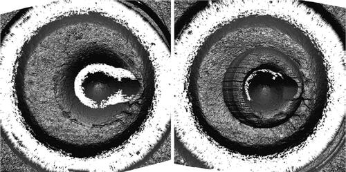
Notice that the image on the right has marks (“striations”) around the indentation in the center of the cartridge case (“firing pin impression”). These marks are called “aperture sheer,” and firearm examiners use them to determine whether the same gun fired two cartridge cases. Notice that the image on the left does not have aperture sheer. Although these cartridge cases were fired by the same gun, in successive order, they contain very different information.

If an examiner—who is unaware of ground truth—compared these two cartridge cases on a test and reported Inconclusive, that would be an error according to the ground truth norm because the same gun fired both cartridge cases. However, according to the Dror and Scurich (2020) approach, that response would not be an error. On the contrary, it would be correct because the lack of quality and quantity of aperture sheer does not justify calling an Identification.

Another example from this same study is comparison Set 17, a same-source comparison. Set 17 contained no striations that could be used to make an identification. As noted by Law and Morris (2021), “the smooth firearm surfaces led to few, if any, reproducible individual characteristics on the fired cartridge cases” (p. 8), and in fact 15 out of the 17 examiners in the study called Inconclusive for this comparison set, even though ground truth is same source.

The essence of the Dror and Scurich (2020) argument is that when an examiner states that a bullet or cartridge case contains an absence of markings (i.e., is inconclusive according to the AFTE definition), there must be a way to evaluate this claim. Doing so is not uncomplicated, given that objective standards for determining the quality and quantity of markings in firearms do not exist. Dror and Scurich (2020) suggested several practical ways to do this in the absence of objective standards. Their proposals engendered debate (Weller and Morris 2020; Biedermann and Kotsoglou 2021; Dror 2022; Scurich 2022; Arkes and Koehler 2022b; 2023). However, assuming there is some acceptable way to evaluate whether evidence is inconclusive, evaluating inconclusive responses on a test becomes straightforward, according to Table 2, adapted from Dror and Scurich (2020).

Table 2 Proposed study design that enables evaluation of inconclusive decisions.

Examiner’s Decision
Evidence	Identification	Elimination	Inconclusive
Same-Source	Correct	Error	Error
Different-Source	Error	Correct	Error
Inconclusive	Error	Error	Correct

2 Signal Detection Theory

Signal Detection Theory (SDT) is a well-known framework for analyzing diagnostic decisions, such as making medical diagnoses, aptitude testing, materials testing, and polygraphy (Swets and Pickett 1982; Swets 1988; Swets, Dawes, and Monahan 2000; 2020). SDT has two parameters, d’ and β. The former—d’—is the difference in means between the signal and noise distribution in standard deviation units and reflects the ability to discriminate between signals and noise. The latter—β—is a decision threshold for classifying inputs as either signal or noise. According to SDT, the accuracy of diagnostic decisions is a function of how well examiners can identify signals relative to noise and how much signal they require before making a decision (Green and Swets 1966; Swets and Pickett 1982). Classification performance is often characterized in terms of sensitivity and specificity. Sensitivity is the proportion of actual signals classified as signals and specificity is the proportion of noise inputs classified as noise.

The primary benefit of the SDT approach is that it allows researchers to plot a Receiver Operating Characteristic (ROC) curve, which provides a measure of performance that is independent of decision thresholds and base rates—factors that are confounded when examining a single false positive error rate (e.g., Wixted and Mickes 2012, 2015). The Area Under the ROC Curve (AUC) (see Hanley and McNeil 1982) is considered to be the optimal performance metric for numerous reasons, which are well summarized by Bowers and Zhou (2019):

First, the meaning of AUC is invariant for different datasets, so a higher value is always better than a lower value. Second, AUC provides a more straightforward statistical interpretation. Third, AUC can calculate confidence intervals, allowing researchers to compute whether two AUCs are significantly different from each other, as we show below in the application examples. Fourth, AUC can compare variables that have some categories dominate over other categories while Kappa cannot handle such variables. Fifth, AUC is robust to skewed data, whereas Kappa calculations can be distorted for skewed data (internal citations omitted, pp. 29–30).

Three recent articles have introduced SDT to the forensic science domain (Smith and Neal 2021; Albright 2022; Arkes and Koehler 2022b). Interestingly, the three analyses have used different approaches to treating inconclusive responses. As mentioned, Arkes and Koehler (2022b) stated that inconclusive responses ought to be dropped from accuracy/error rate calculations. However, they did not explain how this would impact SDT measures of discriminability, such as d’.

Smith and Neal (2021) took a confusing position on how to deal with inconclusive responses in an SDT analysis. After giving a lengthy hypothetical example of SDT in which inconclusive was a response option and was plotted on their ROC curve (Figure 2, p. 323), they write:

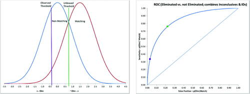
Fig. 2 Left: Displays corresponding PDFs implied by observed sensitivity and specificity omitting inconclusive responses assuming Normal-Normal, equal variance distributions; right: Corresponding ROC curve assuming a Normal-Normal, equal variance model with inconclusive responses omitted.

An inconclusive decision is never a correct decision, but there are clearly instances in which an inconclusive decision is an appropriate decision. From this standpoint, the framework offered by Dror and Scurich is clearly inappropriate for evaluating the correctness of examiners decisions; however, we can see how this framework, or a similar framework, might be useful for assessing the appropriateness of examiners decisions. (p. 329)

Smith and Neal (2021) did not explain how, if at all, SDT is to accommodate their proposed distinction of “correct” versus “appropriate” decisions.

Albright (2022) conducted the most comprehensive SDT analysis. His analysis demonstrated the impact of simply dropping inconclusive responses and how it spuriously inflates performance by discarding a significant amount of data. As a result, Albright proposed a new paradigm for firearm examiners. Rather than make a categorical judgment (e.g., Identification, Inconclusive, or Elimination), examiners would make a binary judgment (i.e., Identification or Elimination) and give a confidence judgment on an 8-point scale. “Inconclusive is not an option” (p. 6). Albright’s formulation leads to a relatively straightforward application of SDT.

Albright’s proposed approach, in which a binary judgment is made along with a confidence rating, is defensible and appropriate for future studies. At the same time, Albright noted his concern that firearm examiners are likely to reject an approach that prohibits inconclusive responses. We agree with this concern. It is possible, however, to use the SDT framework and permit inconclusive responses.

ROC analyses involving three or more diagnostic categories have been developed for medical decision-making (Scurfield 1996, 1998; Edwards and Metz 2006). Examples include a radiologist deciding whether a film displays malignant lesions, benign lesions, or no lesions (Dreiseitl, Ohno-Machado, and Binder 2000) or a psychiatrist determining whether a psychotic patient has affective psychosis, schizophrenia, or a delusional disorder (Mossman 1999; He, Song, and Frey 2008). Although these decision problems could be conceptualized as a binary decision task, doing so “run[s] the risk of distorting the problems’ complexity and difficulty” (Mossman 1999, p. 78). “Three-Way ROCs” were specifically developed for decision problems with three categories and three decision options.

In this article, we introduce the three-way ROC approach and demonstrate its utility within the context of forensic firearms examination. We believe the three-way ROC is better suited to analyze the performance of forensic firearm examiners precisely because inconclusive evidence and inconclusive responses are a reality in applied work. However, first, we present a series of ROC analyses based on actual data from a firearm examiner study (Monson, Smith, and Peters 2023). The previous SDT analyses have relied on hypothetical data. The analyses based on actual data demonstrate why inconclusive responses lead the traditional ROC approach to dubious results and illustrate why the three-way ROC is necessary.

3 Examples of Two-Category SDT Applied to Forensic Firearm Examination

The following analysis uses the results for bullet comparisons from the Monson, Smith, and Peters (2023) study. Table 3 presents the results reported on page 89 of the Monson, Smith, and Peters (2023) study. A few preliminary points should be noted. First, we collapsed the three categories of Inconclusives (INC-A, INC-B, INC-C) into a single category of Inconclusives. This collapsing is consistent with practice in the field (e.g., Best and Gardner 2022). Second, by design of the study researchers, there are about twice as many different source (“nonmatching”) bullet comparisons as same source (“matching”) comparisons. Third, over half (50.6%) of the 4247 bullet comparisons were judged inconclusive.

Table 3 Contingency Table of frequencies of bullets by forensic expert classifications (Monson, Smith, and Peters 2023, p. 89).

Examiner’s Decision
Bullet	ID	Elimination	Inconclusive	Total
Matching	1076	41	288	1405
Nonmatching	20	961	1861	2842
Total	1096	1002	2149	4247

The standard SDT model can only be applied to the data by reducing or collapsing the three judgments of Identification, Elimination, and Inconclusive into two categories. There are three possible approaches:

1. Omit Judged Inconclusives (leaving only Identifications and Eliminations)

2. Combine Eliminations and Judged Inconclusives into a single category

3. Combine Identifications and Judged Inconclusives into a single category

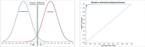
3.1 Omit Inconclusive Responses

The first approach is to omit the Inconclusives column from Table 3, which results in sensitivity = p(Identification | match) = 1076/(1076 + 41) = 0.9633 and specificity = p(elimination | nonmatching) = 961/(961 + 20) = 0.9796. For purposes of this demonstration, we will make the common assumption that the signal and noise distributions are both Normal with equal variances. Additional empirical investigation is required to validate this assumption in the context of forensic firearm examination. Assuming a Normal-Normal equal variance SDT model, d-prime can be calculated: (1) $${\mathrm{d}}^{\prime }\text{=}{\Phi }_{\mathrm{S}}^{-1}\left(\text{Sensitivity}\right)-{\Phi }_{\mathrm{S}}^{-1}\left(1-\text{Specificity}\right)\text{=3}.84$$(1) where ${\Phi }_{\mathrm{S}}^{-1\mathrm{ }}$ is the inverse standard normal cumulative distribution function (Stanislaw and Todorov 1999).

Figure 2 (left) displays corresponding Normal probability density functions (PDFs) (Means $=0\text{ \&}3.84$; SDs =1) with the observed threshold (${\mathrm{T}}_{\mathrm{o}}$) (purple vertical line) corresponding to the empirical sensitivity and specificity. (2) $${\mathrm{T}}_{\mathrm{o}}={\Phi }_{\mathrm{N}}^{-1}\left(\text{Specificity}\right)={\Phi }_{\mathrm{M}}^{-1}\left(1-\text{Sensitivity}\right)=2.05,$$(2) where ${\Phi }_{\mathrm{N}}^{-1}$ is the inverse normal cumulative distribution function for the nonmatching (noise) distribution, and ${\Phi }_{\mathrm{M}}^{-1}$ is the inverse Normal cumulative distribution function for the matching (signal) distribution function (Stanislaw and Todorov 1999).

The observed threshold is only slightly (conservatively) biased. Assuming equal base rates and error penalties, T_u = 1.92, corresponding to $\beta \hspace{1em}=$ 1.0 (green vertical line), corresponding to the intersection of the signal and noise PDFs. The bias parameter (c), defined as the difference between T_o and T_u, is c = 0.13.

Figure 2 (right) displays the associated ROC curve with the observed sensitivity and false-positive rate indicated as a purple dot near the upper left corner. The green dot represents the sensitivity and false-positive rate resulting from using the unbiased (green) threshold in Figure 2 (left).

The Area Under the ROC Curve (AUC) represents the probability that the signal value (plotted on the horizontal axis in Figure 2) is greater for a randomly selected matching bullet than a randomly selected nonmatching bullet (Hanley and McNeil 1982). AUC is also related to the familiar nonparametric Mann-Whitney U-statistic (also known as the Wilcoxon rank-sum test statistic) (AUC = U/n₁n₂) (Hanley and McNeil 1982). The area under the ROC curve in Figure 2 (right) is calculated from d’ (Stanislaw and Todorov 1999): (3) $${\mathrm{A}}_{\mathrm{d}\prime }={\Phi }_{\mathrm{S}}({\mathrm{d}}^{\prime }/2^{\text{1/2}})=\mathrm{0.9967.}$$(3)

As expected, eliminating the difficult cases results in extremely high classification accuracy. Indeed, comparing these values to other contexts in which experts make decisions shows that they are implausible.

Arkes and Mellers 2002 note, “Medical tests provide a benchmark against which we can compare estimates of d’ in legal settings. In medicine, d’s are typically higher, but they still do not exceed 3.0” (p. 633). For example, experts using photomicrographs to test for cervical cancer had a d’ of 1.6, and a computer evaluation of the same material increased d’ to 1.8—both of which are half as large as the 3.84 d’ that results after one drops the inconclusive responses. They note, “These benchmarks show that, even with enormous technological sophistication, it is not easy to achieve levels of d’ that exceed 2” (Arkes and Mellers 2002, p. 634).

3.2 Combine Eliminations and Inconclusive Responses into a Single Category

The second approach combines Eliminations and Inconclusives into a single category and compares them to Identifications. In effect, the decision is Identification or Not an Identification. This approach is akin to a criminal trial: a defendant is either convicted or found not guilty. However, not guilty does not mean innocent; only that the evidence was insufficient to convict. Similarly, “not an identification” does not mean different guns fired the bullets; only that the examiner did not judge the markings sufficiently similar to make an identifi-cation.

The collapsed data in Table 3 result in sensitivity (p(Identification | match) = 1076/(1076 + 41 + 288) = 0.7658 and specificity (p(not Identification | nonmatching) = (961 + 1861)/(961 + 1861 + 20) = 0.9930. Using the same assumptions and equations for approach 3.1, that is, a Normal-Normal equal variance SDT model, d’ = 3.18. Figure 3 (left) displays the corresponding Normal PDFs (Means = 0 & 3.18; SDs = 1) with the threshold (purple vertical line, T ${}_{\mathrm{o}}=2.46$) corresponding to the observed sensitivity and specificity. Note that this threshold is substantially biased; assuming equal base rates and error penalties, the unbiased threshold would be T ${}_{\mathrm{u}}=1.59$ (green vertical line), with bias (c) = 0.87. The observed threshold suggests that nonmatching cases are perceived as more likely than matching cases or a perceived greater penalty for false positives (identifying bullets that are nonmatching) than for false negatives (not identifying bullets that are matching).

Fig. 3 Left: PDFs implied by observed sensitivity and specificity from combining inconclusive responses and Eliminations, assuming Normal-Normal, equal variance distributions; right: Corresponding ROC curve assuming a Normal-Normal, equal variance model for Identification versus no Identification (inconclusive responses and Eliminations combined).

Figure 3 (right) displays the associated ROC curve with the observed sensitivity and false-positive rate indicated as a purple dot. The green dot represents the sensitivity and false-positive rate from using the unbiased threshold plotted in Figure 3 (left). Using the biased threshold reduces the hit rate for identifying matching bullets from 95% to 77%. The area under the ROC curve in Figure 3 (right), calculated from d’, is A ${}_{\mathrm{d}\prime }=0.9877$. Classification accuracy is somewhat attenuated compared to omitting the cases judged Inconclusive, but it is still extremely high (d’ > 3.0). This extremely high classification accuracy is partly an artifact of the experimental study design: the ratio of nonmatching to matching comparisons is 2:1, and there are effectively two ways for examiners to get a correct response for nonmatching comparisons (either Elimination or Inconclusive).

3.3 Combine Identifications and Inconclusive Responses into a Single Category

The third approach combines Identifications and Inconclusive responses into a single category and compares it to Eliminations. In effect, the judgment is either Elimination or not Elimination. The focus here is on the ability of examiners to screen out nonmatching bullets. Medicine uses screening tests to eliminate individuals without risk factors before more expensive and resource-intensive diagnostic tests are conducted. Being “screened in” does not indicate that an individual does have the disorder, only that additional testing is warranted. Similarly, a judgment of “not elimination” does not mean that the same gun fired the bullets, only that further examination is warranted.

The collapsed data in Table 3 results in sensitivity (p(Eliminated | nonmatching) = 961/(961 + 20 + 1861) = 0.3381 and specificity (p(not Eliminated | matching) = (1076 + 288))/(1076 + 288 + 41) = 0.9708. Using the same assumptions and equations for cases 3.1 and 3.2, d’ = 1.48. Figure 4 (left) displays the corresponding Normal PDFs (Means = 0 & 1.48; SDs = 1) with the threshold (purple vertical line, T ${}_{\mathrm{o}}=-0.42$) corresponding to the observed sensitivity and specificity. Note that this threshold is substantially biased (c = 1.16); assuming equal base rates and error penalties, the unbiased threshold would be T ${}_{\mathrm{u}}=0.74$ (green vertical line). These results reflect a stringent standard for eliminating bullets; most items will not be eliminated, given the observed threshold.

Fig. 4 Left: PDFs implied by observed sensitivity and specificity from combining inconclusive responses and Identifications, assuming Normal-Normal, equal variance distributions; right: ROC curve assuming a Normal-Normal, equal variance model for Eliminated versus not Eliminated (inconclusive responses and Identifications combined).

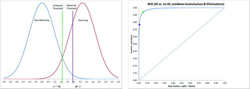
Figure 4 (right) displays the associated ROC curve with the observed sensitivity and false-positive rate indicated as a purple dot. The green dot represents the sensitivity and false-positive rate from using the unbiased threshold plotted in Figure 4 (left), which would eliminate 77% of nonmatching bullets. The observed hit rate for eliminating nonmatching bullets is only about 33%. The area under the ROC curve in Figure 4 (left), calculated from d’, is A ${}_{\mathrm{d}\prime }=0.8516$. Accuracy is substantially attenuated compared to that resulting from simply omitting the cases judged Inconclusive.

4 Example of Three-Way ROC Analysis Applied to Forensic Firearm Examination

None of the three 2-category approaches to retrofitting the traditional SDT approach is satisfactory. Dropping the Inconclusive responses discards an enormous quantity of data and yields implausible values. This approach is all the more troubling given that Inconclusive conclusions made by firearm examiners are unreliable (Dorfman and Valliant 2022b; Baldwin et al. 2023). The other two approaches combine Inconclusive responses with either Identifications or Eliminations. These approaches significantly differ from the task forensic firearm examiners conduct in actual casework, making the resulting performance metrics of limited value. Further, both involve sacrificing information that could—in theory—be used to make an Elimination (when Inconclusive and Identification are combined) or an Identification (when Inconclusive and Elimination are combined).

In short, to the extent examiners are permitted to make Inconclusive decisions, the three-way ROC is necessary to characterize the performance of firearm examiners making comparisons of bullets or cartridge cases. The following section provides an illustrative application of the three-way model based on the data in Table 3.

The three-way ROC approach assumes a category of inconclusive evidence; conceptually, it assumes a 3 × 3 contingency table like that depicted in Dror and Scurich (reproduced above). Unfortunately, no study has yet to include this third category of Inconclusive evidence. Because of this absence of data, and for the sake of demonstration, we applied the following four assumptions to estimate a 3 × 3 table from the data in Table 1. The assumptions are intended to preserve the original data proportions in the Matching and Nonmatching rows of Table 3. The assumptions are:

1. The rate of Inconclusive Evidence matches the overall rate of judged Inconclusives (50.6%)

2. The rate of Inconclusive Evidence from Matching Bullets matches the rate of Matching Bullets judged as Inconclusive (20.5%)

3. The rate of Inconclusive Evidence from Nonmatching Bullets matches the rate of Nonmatching Bullets judged as Inconclusive (65.5%)

4. The frequency of judged Identifications, Eliminations, and Inconclusives for Matching and Nonmatching Bullets remains the same as in Table 1.

Table 4 displays the frequencies applying these four assumptions to the observed frequencies in Table 3, and Table 5 gives each judgment’s associated probabilities relative to the evidence category.

Table 4 Synthetic contingency table of frequencies consistent with the observed frequencies in Table 1 and the four assumptions listed above.

Bullet	ID	Elimination	Inconclusive	Total
Matching	855	33	229	1117
Nonmatching	7	332	642	981
Inconclusive	234	638	1278	2149
	1096	1003	2149	4247

Table 5 Probabilities of judgement (columns) conditional on true category of bullet (rows).

Bullet	ID	Elimination	Inconclusive	Total Freq.
Matching	76.54%	2.95%	20.50%	1117
Nonmatching	0.71%	33.84%	65.44%	981
Inconlusive	10.89%	29.69%	59.47%	2149
Total Freq.	1096	1003	2149	4247

As indicated in Table 5, over three-fourths of the Matching bullets were correctly Identified, about a third of the Nonmatching bullets were correctly Eliminated, and about 60% of the Inconclusives were correctly called Inconclusive (the diagonals of the table). Note that these first two values (i.e., the percentage of correct Identifications and Eliminations, respectively) are identical to the values reported in Table 3, which comes directly from Monson, Smith, and Peters (2023).

We used the synthetic data in Table 3 to construct a three-way SDT model. This model assumes a signal distribution for each of the three bullet categories (Nonmatching, Inconclusive, and Matching). The three distributions were assumed to be Normal with possibly unequal variances. We further assumed that the means were ordered as follows: Nonmatching < Inconclusive < Matching. The signal is assumed to be greatest for Matching bullets and smallest for Nonmatching bullets, with Inconclusives between Matching and Nonmatching. In judging bullet samples, firearm examiners are assumed to have two thresholds, one for distinguishing Eliminations from Inconclusives and the other for distinguishing Inconclusives from Identifications. Inconclusives are conceptualized as having a signal not so strong to warrant an Identification but not so weak to justify an Elimination.

Each row of percentages in Table 3 must sum to 100%; hence, there are two equations implied by each row or six equations in total. Each of the three Normal distributions is defined by two parameters (mean and SD) for six distribution parameters. In addition, the two thresholds are unknown, resulting in eight unknown parameters. Without loss of generality, we set the Nonmatching distribution mean to 0.0 to ensure positive means and the Inconclusive distribution standard deviation to 1.0. Then, we solved for the remaining unknown parameters (four distribution parameters, that is, two means and two sd, and the two threshold parameters (T_E = lower threshold for Elimination and T_I = upper threshold to ID) to match the percentages in Table 3. Finally, we applied iterative numerical methods to solve the following six simultaneous equations for the six unknown parameters (thresholds for Elimination and Identification (T_E & T_I), mean of true inconclusives and matching distributions (µ_I & µ_M), and standard deviations of the nonmatching and matching distributions (${\sigma }_{\mathrm{N}}$ & ${\sigma }_{\mathrm{M}})$: (4) $${\mathrm{T}}_{\mathrm{E}}={\Phi }_{\mathrm{N}}^{-1}\left(\mathrm{p}\left(\text{Elimination} | \text{Non}-\text{matching}\right)\right)\text{=}{\Phi }_{\mathrm{N}}^{-1}(0.338)$$(4) (5) $${\mathrm{T}}_{\mathrm{E}}={\Phi }_{\mathrm{I}}^{-1}\left(\mathrm{p}\left(\text{Elimination} | \text{Inconclusive}\right)\right)\text{=}{\Phi }_{\mathrm{I}}^{-1}(0.297)$$(5) (6) $${\mathrm{T}}_{\mathrm{E}}={\Phi }_{\mathrm{M}}^{-1}\left(\mathrm{p}\left(\text{Elimination}|\text{Matching}\right)\right)={\Phi }_{\mathrm{M}}^{-1}(0.030)$$(6) (7) $${\mathrm{T}}_{\mathrm{I}}={\Phi }_{\mathrm{N}}^{-1}\left(1\text{-}\mathrm{p}\left(\text{ID}|\text{Non}-\text{matching}\right)\right)={\Phi }_{\mathrm{N}}^{-1}(0.992)$$(7) (8) $${\mathrm{T}}_{\mathrm{I}}={\Phi }_{\mathrm{I}}^{-1}\left(1\text{-}\mathrm{p}\left(\text{ID}|\text{Inconclusive}\right)\right)={\Phi }_{\mathrm{I}}^{-1}(0.892)$$(8) (9) $${\mathrm{T}}_{\mathrm{I}}={\Phi }_{\mathrm{M}}^{-1}\left(1\text{-}\mathrm{p}\left(\text{ID} | \text{Matching}\right)\right)\text{=}{\Phi }_{\mathrm{M}}^{-1}(0.235),$$(9) where ${\Phi }_{\mathrm{N}}^{-1},{\Phi }_{\mathrm{I}}^{-1}$, and ${\Phi }_{\mathrm{M}}^{-1}$ are the inverse cumulative normal distribution functions for the Nonmatching, Inconclusive, and Matching distributions.

The resulting means and standard deviations of the six distributions are provided in Table 6.

Table 6 Means and standard deviations of empirical Normal distributions.

Bullet	Mean	Standard Dev
Nonmatching	0.00	0.62
Inconclusive	0.28	1.00
Matching	2.61	1.52

NOTE: Without loss of generality, one location parameter (mean = 0) and one scaling parameter (sd = 1) were fixed.

As expected, the Inconclusive distribution mean is between the means of the Matching and Nonmatching distributions. The difference in means between the Nonmatching and Inconclusive distributions (0.28) is much smaller than the mean difference between the Matching and inconclusive distributions (2.33). The standard deviation of the Nonmatching distribution is 62% of that of the Inconclusive distribution, while the standard deviation of the Matching distribution is 52% larger than that of the Inconclusive distribution.

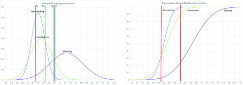
The Normal density functions for these three distributions are plotted in Figure 5 (left). As expected, there is considerable overlap among the three distributions. The two vertical lines are the observed thresholds (T ${}_{\mathrm{E}}=-0.26$ and T ${}_{\mathrm{I}}=1.51$) calculated from (2)–(9), yielding classification probabilities consistent with Table 5 for the Normal distributions defined in Table 6. Bullets with a (subjective) signal value below–0.26 result in Elimination, while bullets with a signal value above 1.51 constitute an Identification. All bullets with a signal between–0.26 and 1.51 are judged as Inconclusive. The corresponding areas under the curves of the Normal plots in Figure 5 (left) match the conditional probabilities of errors and correct classifications in Table 5.

Fig. 5 Left: Plots of Normal densities and thresholds (T_E & T_I, purple) consistent with synthetic 3 × 3 Frequency data. Thresholds T_EU and T_IU (green) represent unbiased Elimination and Identification thresholds to maximize the correct classification percentage assuming equal base rates; right: Cumulative distribution functions consistent with synthetic 3 × 3 Frequency data.

The empirical thresholds derived from the synthetic data in Table 5 indicate an overall correct classification rate of 56.6%, assuming equal base rates (1/3 of all cases) for the three categories. The percentage of correct classifications vary substantially across the three categories: nonmatching (33.8% correct), inconclusives (59.5% correct), and matching cases (76.5%). We calculated unbiased thresholds assuming equal base rates and error penalties, which is equivalent to maximizing the correct classification rate, using the three Normal distributions defined in Table 6 and plotted in Figure 5 (left). The unbiased, correct classification rate is 62.2%, using unbiased thresholds T ${}_{\text{EU}}=0.65$ and T ${}_{\text{IU}}=1.46$, which is 5.6% greater than the observed overall correct classification rate assuming equal base rates. While the upper threshold for Identification classification exhibits only minor bias (c ${}_{\mathrm{I}}=0.05$), the lower threshold for Elimination exhibits substantial bias (c ${}_{\mathrm{E}}=0.91$). The unbiased thresholds yield correct classification percentages of 85.3% (nonmatching), 23.7% (inconclusives), and 77.5% (matching), which dramatically increases correct classifications for nonmatching items and decreases correct classifications for inconclusive items. This bias is consistent with the third approach described above for combining categories, suggesting either that nonmatching items are rare or that misclassifying nonmatching items as either inconclusive or an Identification is less costly than misclassifying Inconclusive or matching items as Elimination.

The Normal cumulative distribution functions corresponding to those described in Table 6 and the densities plotted in Figure 5 (left) are plotted in Figure 5 (right). The correct classifications and error values can be read directly from the points of intersection of the cumulative curves and thresholds, corresponding to the synthetic rates presented in Table 5.

The ROC curve for the usual 2-category SDT can be generalized to a 3-dimensional surface for three-way SDT. The surface is a shell representing correct classification rates for all three categories (nonmatching, inconclusive, and matching) plotted within a unit cube. For example, perfect classification would be represented by the point (1,1,1) indicating 100% correct classification for each of the three categories. The surface is generated by considering all possible pairs of threshold values, T_E < T_I. Figure 6 is a scatterplot of points on the receiver operating surface (ROS) corresponding to the distributions derived in Table 6 and plotted in Figure 5.

Fig. 6 The Receiver Operating surface (ROS).

The 10,000 points plotted in Figure 6 were generated from random pairs of threshold values,–2 < TE < RI < 6. While the surface includes values of the thresholds from +/–infinity, thresholds beyond the range of–2 to 6 yield correct classification percentages near the edges, either 0 or 100%. All possible threshold policies (T_E < T_I) are represented on the surface approximated by the three-dimensional scatterplot. Both the empirically calculated thresholds from the synthetic data in Table 5 and the unbiased thresholds assuming equal base rates and error penalties are represented on the surface plotted in Figure 6.

Much like the area under the ROC curve (AUC) for a binary decision problem (Hanley and McNeil 1982), the three-way ROC has an analogous metric known as the volume under the surface (VUS) that summarizes discrimination performance across the entire range of possible classification thresholds (Mossman 1999). For the regular 2-category ROC, the guessing probability is 1/2 since there are two distributions, thus, only two possible orders. The interpretation of VUS is the probability of drawing one observation from each of the three category distributions that are ordered correctly, that is, Matching signal > Inconclusive signal > Nonmatching signal. For the three-way case, the guessing probability is 1/6 ($\sim 0.17$) since three items were drawn, resulting in six possible orders. That is, guessing would result in one out of six correct orderings of signals drawn from the three distributions.

We used Monte-Carlo simulation to estimate the Volume Under the Surface (VUS) in Figure 6. VUS is estimated to be 0.52 based on 10,000 simulation trials. The estimated VUS is greater than chance (guessing VUS = 0.17) but less than ideal (VUS = 1.0). Note that the value of VUS is independent of the thresholds chosen, represented by a single point on the surface (not unlike the value of AUC in a 2-category SDT being independent of the threshold selected.) To provide additional context to this estimate, Dreiseitl, Ohno-Machado, and Binder (2000) provide a plot directly comparing AUC values to VUS values (Figure 5, p. 328); a VUS of 0.52 corresponds to an AUC of approximately 0.78. As noted above, commentators across disciplines have argued that AUC—and, by implication, VUS, in the case of three-way ROCs—is the optimal performance metric (Bowers and Zhou 2019).

5 Discussion

There are over 10,000 requests annually for a forensic firearm examination in the United States (Durose and Burch 2016). Forensic firearm examiners have testified in court as to their findings for over a century (Garrett et al., in press). Despite the fact that the United States Supreme Court ruling in Daubert (1993) mandated judges to consider the “known or potential rate of error” associated with the technique, it is only in the last decade that tests of firearm examiner performance have been conducted. These studies have engendered significant disagreement about how to properly measure and characterize examiner performance due in large part to the bevy of inconclusive responses in controlled studies.

Inconclusive decisions are a common aspect of firearm examination casework. In one survey, practicing firearm examiners self-reported that 20% of their conclusions in casework are inconclusive (Scurich, Garrett, and Thompson 2022). Indeed, this sample reported inconclusive decisions are more common than eliminations in casework. A different study reported that 40% of casework samples were deemed inconclusive, though the study expressed concerns about the accuracy of this figure (Neuman et al. 2022). Regardless of the exact figure, inconclusive decisions in casework are not trivial, and they are even more frequent in tests of firearm examiners. Furthering our understanding of the theory and process of firearm examination requires the inclusion of inconclusive evidence in tests of examiner performance. Simply put, the performance of forensic firearm examiners cannot be determined without considering their accuracy in judging all three categories of evidence: matching, nonmatching, and inconclusive.

The SDT approach has been applied across numerous scientific domains to study the performance of human decision-makers (Wixted 2020). However, the traditional two-category SDT model is inappropriate for the firearm examiner domain because firearm examiners are not limited to making binary decisions. As demonstrated with actual data from a firearm error rate study, imposing the two-category SDT model leads to implausible results and lacks ecological validity, meaning the performance metrics fundamentally do not reflect performance of casework. Therefore, the three-way ROC approach is necessary to characterize the performance of firearm examiners.

The three-way ROC approach allows one to quantify two separate thresholds for eliminating or for identifying items. Examiners’ judgment data can be used to estimate these thresholds and compare them to normative thresholds derived from considering base rates and relative costs of errors. These empirical thresholds calculated from examiner judgments can also be used to derive implicit error penalties or perceived base rates. Omitting the inconclusive (third) category from analysis ignores their prevalence (> 50%) in recently published studies and the subjectivity in setting thresholds for separating inconclusives from matching and from nonmatching items. The approach is also appropriate for other forensic domains that permit inconclusive decisions, such as forensic document examiners (Hicklin et al. 2022) or fingerprint examiners (Ulery et al. 2011).

We demonstrated how a three-way ROC approach could be applied to firearm examination or any domain where judges can make decisions with n > 2 categories. We emphasize that the values in our demonstration of the three-way approach were synthetic and used for illustrative purposes. Therefore, the performance metrics should not be interpreted literally. Synthetic values are necessary because no firearm error rate study has yet to include inconclusive evidence by design. Until this occurs, inconclusive responses will remain ambiguous, making the performance of firearm examiners indeterminate. However, the three-way ROC approach can easily be applied when and if such studies are conducted.

Notes

Notes

1 An additional approach is to report 1- PPV (positive predictive value) (Hofmann, Carriquiry, and Vanderplas 2021). However, 1-PPV is dependent on the base rate, which is arbitrarily determined in research studies, unknowable in casework, relies on non-scientific determinations (Scurich and John 2012; Thompson et al. 2013), and confounds the performance of the examiner with the base rate (Albright 2022).

References

- AFTE. (2022), “AFTE Range of Conclusions,” available at https://afte.org/about-us/what-is-afte/afte-range-of-conclusions
- Albright, T. D. (2022), “How to Make Better Forensic Decisions,” Proceedings of the National Academy of Sciences, 119, e2206567119. DOI: 10.1073/pnas.2206567119.
- Arkes, H. R., and Koehler, J. J. (2022a), “Inconclusives Are Not Errors: A Rejoinder to Dror,” Law, Probability and Risk, 21, 89–90. DOI: 10.1093/lpr/mgac009.
- Arkes, H. R., and Koehler, J. J. (2022b), “Inconclusives and Error Rates in Forensic Science: A Signal Detection Theory Approach,” Law, Probability and Risk, 20, 153–168. DOI: 10.1093/lpr/mgac005.
- Arkes, H. R., and Koehler, J. J. (2023), “Inconclusive Conclusions in Forensic Science: rejoinders to Scurich, Morrison, Sinha and Gutierrez,” Law, Probability and Risk, 21, 175–177. DOI: 10.1093/lpr/mgad002.
- Arkes, H. R., and Mellers, B. A. (2002), “Do Juries Meet Our Expectations?,” Law and Human Behavior, 26, 625–639. DOI: 10.1023/a:1020929517312.
- Baldwin, D. P., Bajic, S. J., Morris, M. D., and Zamzow, D. S. (2023), “A Study of Examiner Accuracy in Cartridge Case Comparisons Part 2: Examiner Use of the AFTE Range of Conclusions,” Forensic Science International, 349, 111739. DOI: 10.1016/j.forsciint.2023.111739.
- Best, B. A., and Gardner, E. A. (2022), “An Assessment of the Foundational Validity of Firearms Identification Using Ten Consecutively Button-Rifled Barrels,” AFTE Journal, 54, 28–37.
- Biedermann, A., and Kotsoglou, K. N. (2021), “Forensic Science and the Principle of Excluded Middle: “Inconclusive” Decisions and the Structure of Error Rate Studies,” Forensic Science International. Synergy, 3, 100147. DOI: 10.1016/j.fsisyn.2021.100147.
- Bowers, A. J., and Zhou, X. (2019), “Receiver Operating Characteristic (ROC) Area under the Curve (AUC): A Diagnostic Measure for Evaluating the Accuracy of Predictors of Education Outcomes,” Journal of Education for Students Placed at Risk (JESPAR), 24, 20–46. DOI: 10.1080/10824669.2018.1523734.
- Daubert v. Merrell Dow Pharmaceuticals, Inc. (1993), 509 U.S. 579
- Dorfman, A. H., and Valliant, R. (2022a), “Inconclusives, Errors, and Error Rates in Forensic Firearms Analysis: Three Statistical Perspectives,” Forensic Science International. Synergy, 5, 100273. DOI: 10.1016/j.fsisyn.2022.100273.
- Dorfman, A. H., and Valliant, R. (2022b), “A Re-Analysis of Repeatability and Reproducibility in the Ames-USDOE-FBI Study,” Statistics and Public Policy, 9, 175–184. DOI: 10.1080/2330443X.2022.2120137.
- Dreiseitl, S., Ohno-Machado, L., and Binder, M. (2000), “Comparing Three-Class Diagnostic Tests by Three-Way ROC Analysis,” Medical Decision Making: An International Journal of the Society for Medical Decision Making, 20, 323–331. DOI: 10.1177/0272989X0002000309.
- Dror, I. E. (2022), “The Use and Abuse of the Elusive Construct of Inconclusive Decisions,” Law, Probability and Risk, 21, 85–87. DOI: 10.1093/lpr/mgac008.
- Dror, I. E., and Scurich, N. (2020), (“Mis)Use of Scientific Measurement in Forensic Science,” Forensic Science International Synergy, 2, 333–338. DOI: 10.1016/j.fsisyn.2020.08.006.
- Durose, M. R., and Burch, A. M. (2016), “Publicly funded forensic crime laboratories: resources and Services. Bureau of Justice Statistics,” available at: https://bjs.ojp.gov/content/pub/pdf/pffclrs14.pdf.
- Edwards, D. C., and Metz, C. E. (2006), “Analysis of Proposed Three-Class Classification Decision Rules in Terms of the Ideal Observer Decision Rule,” Journal of Mathematical Psychology, 50, 478–487. DOI: 10.1016/j.jmp.2006.05.004.
- Faigman, D. L., Scurich, N., and Albright, T. D. (2022), “The Field of Firearms Forensics is Flawed,” Scientific American.
- Garrett, B. L., Tucker, E., and Scurich, N. (in press), “Judging Firearms Evidence,” Southern California Law Review, 97.
- Glossary of the Association of Firearm and Tool Mark Examiners. (2013), 6th edition. Available at https://afte.org/uploads/documents/AFTE/textunderscoreGlossary/textunderscoreVersion/textunderscore6.091922/textunderscoreFINAL/textunderscoreCOPYRIGHT.pdf
- Green, D. M., and Swets, J. A. (1966), Signal Detection Theory and Psychophysics, New York: Wiley.
- Hanley, J. A., and McNeil, B. J. (1982), “The Meaning and Use of the Area under a Receiver Operating Characteristic (ROC) Curve,” Radiology, 143, 29–36. DOI: 10.1148/radiology.143.1.7063747.
- He, X., Song, X., and Frey, E. C. (2008), “Application of Three-Class ROC Analysis to Task-Based Image Quality Assessment of Simultaneous Dual-Isotope Myocardial Perfusion SPECT (MPS),” IEEE Transactions on Medical Imaging, 27, 1556–1567. DOI: 10.1109/TMI.2008.928921.
- Hicklin, R. A., Eisenhart, L., Richetelli, N., Miller, M. D., Belcastro, P., Burkes, T. M., Parks, C. L., Smith, M. A., Buscaglia, J., Peters, E. M., Perlman, R. S., Abonamah, J. V., and Eckenrode, B. A. (2022), “Accuracy and Reliability of Forensic Handwriting Comparisons,” Proceedings of the National Academy of Sciences of the United States of America, 119, e2119944119. DOI: 10.1073/pnas.2119944119.
- Hofmann, H., Carriquiry, A., and Vanderplas, S. (2020), “Treatment of Inconclusives in the AFTE Range of Conclusions,” Law, Probability and Risk, 19, 317–364. DOI: 10.1093/lpr/mgab002.
- Kaye, D. H., Antill, G., Emmerich, E., Ishida, C., Lowe, M., and Perler, R. (2022), “Toolmark-Comparison testimony: A report to the Texas Forensic Science Commission,” available at: https://papers.ssrn.com/sol3/papers.cfm?abstract/_id=4108012
- Law, E. F., and Morris, K. B. (2021), “Evaluating Firearm Examiner Conclusion Variability Using Cartridge Case Reproductions,” Journal of Forensic Sciences, 66, 1704–1720. DOI: 10.1111/1556-4029.14758.
- Monson, K. L., Smith, E. D., and Bajic, S. J. (2022), “Planning, Design and Logistics of a Decision Analysis Study: The FBI/Ames Study Involving Forensic Firearms Examiners,” Forensic Science International: Synergy, 4, 100221. DOI: 10.1016/j.fsisyn.2022.100221.
- Monson, K. L., Smith, E. D., and Peters, E. M. (2023), “Accuracy of Comparison Decisions by Forensic Firearms Examiners,” Journal of Forensic Sciences, 68, 86–100. DOI: 10.1111/1556-4029.15152.
- Mossman, D. (1999), “Three-Way ROCs,” Medical Decision Making: An International Journal of the Society for Medical Decision Making, 19, 78–89. DOI: 10.1177/0272989X9901900110.
- Neuman, M., Hundl, C., Grimaldi, A., Eudaley, D., Stein, D., and Stout, P. (2022), “Blind Testing in Firearms: Preliminary Results from a Blind Quality Control Program,” Journal of Forensic Sciences, 67, 964–974. DOI: 10.1111/1556-4029.15031.
- Scurfield, B. K. (1996), “Multiple-Event Forced-Choice Tasks in the Theory of Signal Detectability,” Journal of Mathematical Psychology, 40, 253–269. DOI: 10.1006/jmps.1996.0024.
- Scurfield, B. K. (1998), “Generalization of the Theory of Signal Detectability to n-Event m-Dimensional Forced-Choice Tasks,” Journal of Mathematical Psychology, 42, 5–31. DOI: 10.1006/jmps.1997.1183.
- Scurich, N. (2022), “Inconclusives in Firearm Error Rate Studies Are Not “a Pass,” Law, Probability and Risk, 21, 123–127. DOI: 10.1093/lpr/mgac011.
- Scurich, N., and Dror, I. E. (2020), “Continued Confusion about Inconclusives and Error Rates: Reply to Weller and Morris,” Forensic Science International. Synergy, 2, 703–704. DOI: 10.1016/j.fsisyn.2020.10.005.
- Scurich, N., Garrett, B. L., and Thompson, R. M. (2022), “Surveying Practicing Firearm Examiners,” Forensic Science International: Synergy, 4, 100228. DOI: 10.1016/j.fsisyn.2022.100228.
- Scurich, N., and John, R. S. (2012), “Prescriptive Approaches to Communicating the Risk of Violence in Actuarial Risk Assessment,” Psychology, Public Policy, and Law, 18, 50–78. DOI: 10.1037/a0024592.
- Smith, A. M., and Neal, T. M. (2021), “The Distinction between Discriminability and Reliability in Forensic Science,” Science & Justice: Journal of the Forensic Science Society, 61, 319–331. DOI: 10.1016/j.scijus.2021.04.002.
- Stanislaw, H., and Todorov, N. (1999), “Calculation of Signal Detection Theory Measures,” Behavior Research Methods, Instruments, & Computers: A Journal of the Psychonomic Society, Inc, 31, 137–149. DOI: 10.3758/bf03207704.
- Swets, J. A. (1988), “Measuring the Accuracy of Diagnostic Systems,” Science, 240, 1285–1293. DOI: 10.1126/science.3287615.
- Swets, J. A., Dawes, R. M., and Monahan, J. (2000), “Psychological Science Can Improve Diagnostic Decisions,” Psychological Science in the Public Interest: a Journal of the American Psychological Society, 1, 1–26. DOI: 10.1111/1529-1006.001.
- Swets, J. A., and Pickett, R. M. (1982), Evaluation of Diagnostic Systems: Methods from Signal Detection Theory, New York: Academic Press.
- Thompson, W. C., Vuille, J., Biedermann, A., and Taroni, F. (2013), “The Role of Prior Probability in Forensic Assessments,” Frontiers in Genetics, 4, 220–223. DOI: 10.3389/fgene.2013.00220.
- Ulery, B. T., Hicklin, R. A., Buscaglia, J., and Roberts, M. A. (2011), “Accuracy and Reliability of Forensic Latent Fingerprint Decisions,” Proceedings of the National Academy of Sciences of the United States of America, 108, 7733–7738. DOI: 10.1073/pnas.1018707108.
- Weller, T. J., and Morris, M. D. (2020), “Commentary on: I. Dror, N Scurich “(Mis) Use of Scientific Measurements in Forensic Science,” Forensic Science International: Synergy, 2, 701. DOI: 10.1016/j.fsisyn.2020.08.006.
- Wixted, J. T. (2020), “The Forgotten History of Signal Detection Theory,” Journal of Experimental Psychology. Learning, Memory, and Cognition, 46, 201–233. DOI: 10.1037/xlm0000732.
- Wixted, J. T., and Mickes, L. (2012), “The Field of Eyewitness Memory Should Abandon Probative Value and Embrace Receiver Operating Characteristic Analysis,” Perspectives on Psychological Science: a Journal of the Association for Psychological Science, 7, 275–278. DOI: 10.1177/1745691612442906.
- Wixted, J. T., and Mickes, L. (2015), “ROC Analysis Measures Objective Discriminability for Any Eyewitness Identification Procedure,” Journal of Applied Research in Memory and Cognition, 4, 329–334. DOI: 10.1016/j.jarmac.2015.08.007.