Statistical Fallacies in Claims about “Massive and Widespread Fraud” in the 2020 Presidential Election: Examining Claims Based on Aggregate Election Results

Abstract

Years after the election, a substantial portion of the electorate, including a significant majority of Republican voters and numerous Republican officials, continue to believe that the 2020 election was stolen. This essay reviews claims of alleged massive electoral fraud in the 2020 U.S. presidential election. These claims are based on analyses of aggregate-level election data. Although the underlying data in each of the 13 claims we review are accurately described, our review reveals that the interpretations of the election data, which suggest massive fraud, are based on invalid statistical or illogical reasoning. In summary, the conclusions about fraud derived from these statistical analyses are categorically incorrect. We believe this article will serve as a valuable educational tool for the press, the public, and students. It underscores the dangers of misusing statistical inference and emphasizes the importance of accurate statistical analysis in political discourse. By discussing statistical fallacies in a nontechnical manner, we aim to make our critiques accessible to a broad, nonspecialist audience. This significantly contributes to the understanding of misinformation and its impact on democracy and public trust in electoral processes. Supplementary materials for this article are available online.

Keywords:

• Elections
• Misinformation
• Statistics

1 Introduction

After the 2020 U.S. presidential election, the losing candidate, Donald Trump, claimed that he had been the victim of massive voter fraud that denied him the election.¹ But these claims were false: “President Trump was advised by his own experts and the Justice Department that his election fraud allegations were false, and he knew he had lost virtually all the legal challenges to the election, but he nevertheless engaged in a successful but fraudulent effort to persuade tens of millions of Americans that the election was stolen from him” (Thompson et al., 2022, p. 100).

In 2020, many Republican members of Congress, state attorneys general, and other Republican office holders endorsed the claim of massive election fraud in 2020—a claim which Trump’s supporters continue to reiterate. Tens of millions of voters, including a clear majority of Republicans and nontrivial numbers of independents and Democrats believed after the election that there was massive fraud in 2020 (Solender, 2020; Gardner, 2021; UMass Amherst, 2021).² Even before the 2020 election a nontrivial proportion of voters believed that most elections are rigged (Zorn, 2017). The claim that Donald Trump lost the 2020 election only because of election fraud continues to be reiterated and believed by many voters (Jacobson, 2023). In the 2022 primaries, some Republican candidates made the assertion of massive election fraud in 2020 a fundamental part of their election platform. Many of those candidates won their primary, and several will be able to affect future election administration in their states after winning in 2022 (Medina, Epstein, and Corasaniti, 2022).³ In October of 2023, the Republican majority in the U.S. House of Representatives selected a Speaker who was the engineer of a legal effort to overturn the election (Waldman, 2023) and voted on January 6, 2021 to decertify the votes of millions of Americans (Yourish, Buchanan, and Denise, 2021).

Thus, not only have claims about 2020 election fraud remained politically salient, but the persistence of voter beliefs in these claims, and the deep partisan divide about them leading to affective polarization, have frightening implications for the prospects of democratic breakdown in the United States (Grofman, 2022; Homans and Peterson, 2022; Leonhardt, 2022). Poll workers and election officials report drastic increases in intimidation and harassment, and fear for their safety (Edlin and Norden, 2023). Most alarmingly, a significant proportion of Americans support the idea of using violence to address political failures.⁴

The supposed evidence supporting massive election fraud comes in many forms, including personal affidavits alleging fraud in particular precincts (McClallen, 2021), to videos allegedly showing direct evidence of vote tampering by poll workers (Gray, 2020), to how-to-videos showing the supposed ease of manipulating the record of votes produced by voting machines or mail ballots including claims about a conspiracy by a particular voting machine vendor (Sganga, 2022), to assertions that more voters voted than were on the jurisdiction’s electoral roll (Ayyadurai, 2020; Swenson, 2020), to statistical claims of the kind rebutted in the present essay. When various courts reviewed claims about election fraud in the period just after the 2020 presidential election involving litigation brought by former President Trump or his supporters, it found no evidence supporting claims of fraud sufficient to change election results, and almost no evidence of fraud of any kind.⁵ But three years after the presidential elections (ca. November 2023), claims about election fraud continue to be litigated in courts in cases alleging that former President Trump and some of his allies were part of a conspiracy that knowingly raised false claims of massively election fraud.⁶

Along with what have been demonstrated in courts to be unsubstantiated claims of observed fraud based on supposed eyewitness testimony or unsubstantiated claims about the manipulation of ballot recording technology,⁷ the types of statistical claims we consider in this essay have been used to support conspiracy theories.⁸ These allegations regarding the 2020 election are propagated as part of what we would call the “Big Lie”. That lie, if believed, fundamentally undermines the democratic bedrock of the United States.

This article seeks to consolidate a set of existing critiques of statistical claims into a single compendium and to reframe these rebuttals in a consistent framework that is accessible to a general audience. Our scope is deliberately limited. We deal solely with claims about fraud that are grounded, at least in part, on indisputable facts about statistical features of the 2020 presidential election, and comparisons of its outcomes to those of previous presidential elections or to other 2020 elections. Another way in which this essay is tightly focused is that we do not seek to argue about what state or federal courts should or should not have decided about election law in the cases brought before them in 2020.

Despite the implausibility of a massive multi-state conspiracy, the volume and variety of claims make them it almost impossible to successfully rebut all of them to a given voter’s satisfaction.⁹ Moreover, the fact that many of these claims about massive fraud in 2020 (including most of those we discuss in this essay) are plausible on their face, even though fallacious, make them harder to refute. Also, there is the mesmerizing power of repetition (Pennycook, Cannon, and Rand, 2018; Vellani et al., 2023); the claim of massive fraud in 2020 is stated ad nauseam in conservative media sources and by former President Trump and his allies.¹⁰ Factual claims are often repeated even after clear contrary evidence has been presented (Hsu and Thompson, 2022).

Exploring why voters believe what they do is not the purpose of this essay.¹¹ Moreover, in this essay we will not discuss the vast bulk of claims about fraud in 2020, namely those that rest on contested facts. Our concern here is a narrowly focused but important one, looking at fallacies of logic and misuse of statistics in claims based on real and undisputed data. Our goal is not to provide new insights about these logical and statistical fallacies. Rather, our goal is put together in one place a useful compendium of many of the most glaring recent misuses of statistical reasoning as applied to understanding elections,¹² and to do so in a way that is readily accessible to nontechnical readers.¹³

We believe strongly that a discussion of statistical fallacies based on real-world examples should be part of any statistics or public policy curriculum. Moreover, these statistical claims have been propagated by a range of influential actors seeking to further the conspiracy theory about the 2020 election, and even been brought up in legal contexts. The widespread acceptance of such claims by the public may further erode democracy by fostering distrust in the legitimacy of American electoral institutions and democratic governance (Norris, 2023). See Table 1 for an inventory of the types of claims we review.

Table 1 Statistical fallacies evaluated from the 2020 election.

Type	Examples
Arithmetic fallacies	Cherry-picking the data Failing to weight units Changes in support among demographic subgroups Two-party vote share versus shares of total votes cast
Misinterpreting statistical significance	False causality Timing mirage
Meretricious probabilistic reasoning	Double voting Benford’s law Tip of the iceberg fallacy Straw man fallacy
Logically invalid arguments with a true premise involving historical election results comparisons	Spoiled ballots
Logically valid arguments with a false premise involving historical election results comparisons	Presidential coattails Bellwether counties Other cross-election comparisons
Logically valid arguments with false statistical premises using comparisons based on features or components of the same presidential election	Split ticket voting versus straight ticket voting Comparison of differences involving samples with different means Matching design (split ticket voting versus straight ticket voting) Matching design (within-election comparisons of areas with and without fraud claims)

Box 1. Media

It was impossible not to be constantly reminded about the fraud claims regardless of which media sources one followed. Virtually every claim made in the conservative press alleging election fraud was given considerable space in the mainstream media, followed by a rebuttal that often went on longer than the statement of the claim. For example, claims that a particular election had more voters than were registered were subsequently rebutted by showing that the list of eligible voters used for the comparison was incomplete (Reality Check team, 2020). And there were follow-up pieces in the mainstream press repeating multiple claims of fraud and their rebuttals, sometimes drawing on social science analysis such as the discussion of fallacious assertions about voting machine vulnerability to fraud (Eggers, Garro, and Grimmer, 2021). In the Washington Post, President Trump had previously been given tens of thousands of Pinocchio points based on other kinds of claims he made found by the Post to be untruthful, with points added every time the claim was repeated (Kessler, 2020). This constant drumbeat about Trump’s factual misstatements and deceitfulness by a source that conservative voters did not trust may simply have reinforced the view among these voters that Trump was telling truths that the mainstream press was determined to hide. Relevant in psychological terms is the aphorism that “the lady doth protest too much,” in which repeated assertions that a given allegation is untrue become taken as support for a belief that it probably is true.

We begin our portfolio of fallacies (see Table 1) with (a) arithmetic fallacies of a simple sort, such as drawing conclusions from unweighted averages where use of weighted average was required, cherry-picking the data to emphasize only those facts that lead to the desired conclusion, and confusing percentages and percentage point changes. Then we discuss (b) improper use of statistical significance, and then turn to (c) inaccurate probabilistic reasoning, such as improperly using as an indicia of fraud having voters with the same name and date of birth. Then we discuss (d) syllogistic arguments based on cross-election statistical comparisons that are either fallacious in form, or that have at least one premise that is indubitably false, and thus which give rise either to invalid or unfounded conclusions. Finally, we briefly consider similar types of statistical errors in (e) syllogistic arguments based on within-election comparisons. Though we certainly do not claim that we have identified every fallacious claim about 2020 that fits within our classification scheme, we believe we have a typology that includes the most common errors involving analysis of aggregate election data.

2 Fallacious Statistically Based Claims about Massive Fraud in the 2020 Presidential Election

2.1 Arithmetic Fallacies

2.1.1 Cherry-Picking the Data

The most primitive form of failing to weigh the data properly is cherry-picking the data to emphasize only those facts that lead to the desired conclusion. In presenting only some facts, a claimant can appear to have been honest while suppressing pertinent information that otherwise would prove their claims either false or incomplete. Because the data being cited are accurate, cherry-picking can prove a persuasive tool.

A standard way to cherry pick 2020 election data to show the potential for fraud is to focus on racial or demographic groups and to highlight the situations where Biden did worse than Clinton (who were both Democratic challengers to Trump). For example, Biden won fewer counties than Clinton. You can also get even more specific, for example, Trump won a greater share of the vote in the city of Philadelphia in 2020 than he did in 2016; and you can find other big cities where Biden underperformed Clinton. In these cherry-picked examples, Biden did less well against Trump than did the previous Democratic candidate and, since Trump beat Clinton, absent fraud, the implicit (and often explicit) conclusion is Trump must also have beaten Biden. But, of course, while there were some urban areas where support for Biden was lower than for Hillary Clinton, there were also urban areas where support for Biden was higher than for Hillary Clinton. Similarly, as discussed below, it is true that in terms of percentage voting for the Democratic candidate, racial minority support for Biden was (marginally) lower than for Hillary Clinton, and Trump did better among rural voters in 2020 than he did in 2016. However, support among categories of white voters, namely the college-educated and those living in suburbs, was higher for Biden than for Hillary Clinton. And there are many more voters living in suburban residences than in rural areas.

It is, of course, the combination of all the subgroup patterns of voting and the (changes) in their sizes across elections that matters for the total popular vote. To reiterate the obvious, looking only at some subsets of voters, or only some geographic areas, for example, only rural counties, is misleading and can lead to ridiculous claims that the candidate who received more votes did not actually receive more votes.¹⁴

2.1.2 Failing to Weight Units

There were various instances of this type of error in discussions of the 2020 election. We first focus on the most common instance. Failing to recognize that large changes in one direction in small population subsets or small population demographic subgroups can be compensated for by small changes in the other direction in large population subsets or demographic units is a common mistake.

It was observed that Trump won more counties in 2020 than he did in 2016, with the implication being that he must have done better in 2020 than in 2016 (Swenson, 2021). But this ignores the number of people in each county. Counties Trump did worse in, though fewer in number, had more voters in them. In the 19 most populous counties, Biden received 7,360,531 more votes than Trump (Biden also won a slight majority in the smallest 3134 counties, but by only 52,640 votes). In fact, in Los Angeles County, Biden netted an additional 609,000 more votes in 2020 than Clinton did in 2016. Out of the over 3000 counties in the United States,¹⁵ the largest 150 contained half of the total votes cast. Biden won 125 of those 150 (83.3%) (see Figure 2).

Fig. 1 Truth social post by former President Donald Trump re the lengths he would be prepared to go to overturn the 2020 election results.

Note: Post accessed June 16, 2023. https://truthsocial.com/@realDonaldTrump/posts/109449803240069864

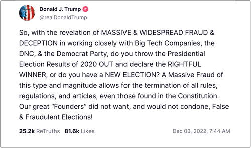
Fig. 2 Votes in each county.

Note: One bar per county. Counties are ordered on the x-axis by the number of voters in each county. Most counties have very few voters (long tail on the left of the plot). Among small and modestly populated counties, Trump won a majority in most; among those with the largest populations, Biden won a majority. Even in the largest counties, there are plenty of Trump voters, and in the smallest counties, there are some Biden voters. The bottom panel shows the cumulative vote across all counties, ordered the same way as the top panel.

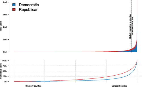
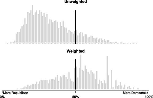
Errors in using unweighted averages when it is appropriate to use a weighted average can be plotted in several ways. Figure 2 presents a dual perspective in a single plot. The upper section illustrates the distribution of votes across counties, arranged on the x-axis from the county with the least to the most votes. It displays the total votes garnered by each candidate, depicted in a stacked manner. Concurrently, Figure 2 traces the progressive accumulation of votes for each candidate, highlighting how Trump is amassing his total vote count at a swifter pace compared to Biden. Also consider histograms that shows the 2020 presidential vote share for each county. When plotted without any reference to the number of voters in each county (Figure 3, top plot; “Unweighted”), it appears that Trump won an overwhelming landslide in the 2020 election. However, if you represent the number of voters by making the height of the bar reflect the number of votes in each county (Figure 3 bottom plot; “Weighted”), we can now see how Biden received a larger share of the total vote.

Fig. 3 Histogram of the 2020 presidential election results, by county.

Note: Both histograms consist of one bin (x-axis) each representing the Democratic share of the vote, from 0% to 100%. The top histogram shows that the majority of counties preferred Trump to Biden. (Bars include the count of counties in each bin) The bottom histogram corrects the bars so that they reflect both the number of counties in each bin, and the number of votes in each county.²⁰ The skew is much more pronounced in the top histogram (giving the incorrect assumption that the country was heavily pro-Trump) and more approximately normal in the bottom (reflecting the true nature of the close election).²⁰The top panel is a simple histogram. To create the bottom panel, line heights are adjusted such that the vote percentage in a county is repeated for each voter in the county, so larger counties are reflected with larger bins.

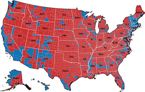
Next, consider a choropleth map of election results by county (Figure 4). As Chief Justice Earl Warren famously quipped in Reynolds v. Sims (1964), “legislators represent people, not trees or acres.” Trump certainly won more acres, but he did not win more voters. If you look at a map of U.S. counties showing those won by President Trump in red and those by Hillary Clinton (or Joe Biden) in blue, you will see a sea of red and only a relative handful of pockets of blues. But those pockets (mostly big cities) have lots of voters in them. Figure 4 depicts the 2020 election with an overwhelming number of counties colored red, indicating Trump won those counties. It does not indicate the number of votes each county, or the margin the winning candidate won.

Fig. 4 Choropleth plot, 2020 presidential election by county.

Note: This choropleth map shows the 2020 Presidential election results by county. Each county is shown using the Albers projection.

Biden won 556 counties (receiving 59,019,426 votes in those counties). In those same 556 counties, Trump received 25,455,244 fewer votes (Trump received 33,564,182 votes in those counties).¹⁶ Trump won 2595 counties (received 40,644,014 votes in counties). In those 2595 counties, Biden received 18,398,446 fewer votes (Biden received 22,245,568 votes in those counties). Thus, Biden had 25,455,244 more votes in counties he won, versus Trump’s 18,398,446 vote advantage in counties he carried (see Table 2). Moreover, to further confound simple calculations, it is helpful to remember that the county with the most Republican votes anywhere in the United States was Los Angeles County, California. Trump received 1,145,530 votes there, although that number was dwarfed by Biden’s 3,028,885.¹⁷ In fact, Trump’s 10 largest county vote totals in 2020 come in counties won by Biden.

Table 2 Popular vote in counties carried by each candidate.

	Biden counties	Trump counties
Biden votes	59,019,426	22,245,568
Trump votes	33,564,182	40,644,014
Difference (pro-Trump)	$-25,455,244$	$+18,398,446$

NOTE: Each candidate received many votes in counties they did not carry. Still, in aggregate, Biden received far more votes overall.

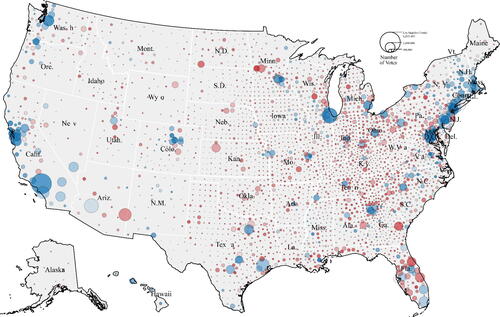
When counties are instead represented on a map in proportion to their votes, such as with a cartogram—a map that has been resized so the units’ area is weighted to its population or some other numeric quantity—it becomes clear that the 2020 election was close, and certainly not an overwhelmingly “red” country shown by a county-level election map.¹⁸ Similarly, in the context of unequally sized units, a “bubble map” can be especially useful (see Figure 5). But it is still virtually impossible to visually sum-total results from a cartogram or bubble map to determine an election winner, especially when the number of units (say counties) is large.¹⁹

Fig. 5 Bubble plot, 2020 presidential election by county.

NOTE: This bubble map shows a vote-weighted representation of the 2020 election. It describes three simultaneous variables: the winner of the county, the number of votes cast, and the number of votes the county was won by. Counties colored in blue were won by Joe Biden, and those colored in red were won by Donald Trump. The size of the circle indicates the number of votes cast. The opacity indicates what the margin of victory was. Because the bubbles overlap, it can be hard to see the densest areas with many counties.

Exit polls suggest an improvement in Trump’s performance from 2016 to 2020 (see Table 3). Despite this apparent enhancement, Trump transitioned from a victorious 2016 campaign to a loss in 2020, with a notable decline in his share of the popular vote. In the 2020 election, Biden garnered 81.2 million votes, accounting for 51.3% of the popular vote, a significant increase from Clinton’s 65.8 million votes (48.2%) in 2016. Trump, on the other hand, secured 74.2 million votes (46.8% of the popular vote) in 2020, up from his 63 million votes (46.1%) in 2016. To understand Trump’s loss despite ostensibly improved exit poll results, we examine three key factors: (a) shifts in the electorate’s composition, (b) the impact of a decrease in third- and fourth-party voting, and (c) changes in geographic support influencing the electoral college outcome.

Table 3 2016 and 2020 exit polls, by race.

2016	White	Black	Latino	Asian	Other racial/ethnic groups
	70%^21	12%	11%	4%	3%
Clinton	37%	89%	66%	65%	56%
Trump	57%	8%	28%	27%	36%
24,537 total respondents
2020	White	Black	Latino	Asian	Other racial/ethnic groups
	67%	13%	13%	4%	4%
Biden	41%	87%	65%	61%	55%
Trump	58%	12%	32%	34%	41%
15,590 total respondents

NOTE: Exit Polls conducted by Edison Research for the National Election Pool.

2.1.3 Changes in Support among Demographic Subgroups

Analyzing the distribution of votes across major political parties and various demographic groups reveals key insights into President Trump’s support patterns. In the 2020 election, Trump saw an increase in support from all racial groups, including Whites, Blacks, Hispanics, Asians, and Others, compared to 2016. These increases are in both raw votes (absolute) and in terms of percentages (relative). Notably, his share of the Black vote rose to 12% in 2020 from 8% in 2016, while his Hispanic vote share grew by four percentage points, reaching 32%, and the Asian share increased from 27% in 2016 to 34% in 2020. Trump also gained a slightly greater share of the White vote in 2020 (58%) than he did in 2016 (57%).

Despite these gains, Trump lost the 2020 election, a larger defeat than his 2016 loss to Clinton. This outcome prompts the question: why did Trump not perform better in 2020 if his 2020 performance is superior to his 2016 performance in each racial/ethnic category? This puzzle has the same form as a well-known result in statistics called Simpson’s Paradox. As explained in the Stanford Encyclopedia of Philosophy “Simpson’s Paradox is a statistical phenomenon where an association between two variables in a population emerges, disappears or reverses when the population is divided into subpopulations.”²⁰ Here we get one result overall (Biden doing better), but opposite results (Trump doing better) when we look at results in each racial/ethnic category, where these form a set of logically exhaustive and mutually exclusive groups. However, the explanation for this puzzle has one element distinct from those used to explain occurrences of Simpson’s. In addition to the need to weight averages by the size of the group—with the relative sizes of the groups changing between 2016 and 2020, we also have the need to distinguish share of the total votes cast from shares of the two-party vote.

To understand Biden’s victory over Trump, it’s crucial to unpack the changes in the electorate’s composition (see Table 3). Notably, while Trump saw an increase in support from minority voters, both in absolute figures and in percentage terms, Biden’s significant advances among White voters, a larger demographic, effectively offset Trump’s gains among minorities. Additionally, despite Trump’s relative increase among minority voters, Biden surpassed Clinton’s absolute performance among these groups. This was due in part to the expanded pool of minority voters in 2020.

According to exit polls, White voters comprised 67% of the electorate in the 2020 election, a decrease from 70% in the previous election. In the 2016 election, non-Hispanic Whites contributed 54.3 million votes to Trump’s tally (57% of his total votes), while Clinton garnered 35.2 million votes from this group (37% of her total vote). By 2020, Trump’s support among White voters had risen to 61.6 million (58% his total votes). In contrast, Biden received 43.5 million votes from White voters (41% of his total votes). This change marked a notable shift, with Biden gaining more White votes than Trump compared to their 2016 performance (as detailed in Table 4). Notably, White voters were Trump’s strongest demographic in both elections, despite their shrinking share of the electorate.

Table 4 Change in non-Hispanic White votes between 2016 and 2020.

	2016	2020	Difference
Trump	54,531,026 (57%)	61,565,755 (58%)	$+7,034,729$
Clinton/Biden	35,397,332 (37%)	43,520,620 (41%)	$+8,123,288$
Other	5,740,108 (6%)	1,061,479 (1%)	$-4,678,629$
Non-Hispanic White votes	95,668,466 (70%)	106,147,853 (67%)	$+10,479,387$
Minority botes	41,000,771 (30%)	52,281,778 (33%)	$+11,281,007$
All votes	136,669,237	158,429,631	+21,760,394

NOTE: The White proportion of the total votes cast was 70%. In 2020, it was 67%. Data from CNN Exit Polls, 2016, 2020. Data are estimated.

Another critical factor was the overall increase in voter turnout in 2020. The number of non-Hispanic White voters rose from approximately 95 million in 2016 to about 106 million in 2020, while minority voter numbers grew from 40.8 million to 52.2 million (see Table 4). This change resulted in the proportion of minority voters within the electorate increasing from roughly 30% in 2016 to 33% in 2020, and a decrease of the White proportion of the electorate. Although Trump improved his performance among White voters compared to Clinton in 2016, Biden’s gain within this demographic was more significant, underscoring the pivotal role of voter demographics and turnout in the 2020 election outcome.

In sum, Trump’s support among minority voters increased both in absolute numbers and proportionally. However, Biden’s gains among the larger group of White voters, and the shrinking overall size of the White electorate, counterbalanced Trump’s improvements. Moreover, despite Trump’s gains among minority voters, Biden outperformed Clinton in this demographic due to the increased number of minority voters in 2020.

2.1.4 Two-Party Vote Share versus Shares of Total Votes Cast

Two-party vote share is distinct from total vote shares, and this is crucial for understanding changes in electoral support. Exit polls and other sources of election results often do not display data in terms of the two-party vote share, leading to the combined Democratic and Republican shares not necessarily totaling 100%. This distinction is key in understanding the shift from 2016 to 2020, especially in the context of votes for minor party candidates. The shift in voter support for major party candidates significantly contributed to Biden’s improved performance over Clinton. It also sheds light on Biden’s increased share of the White vote, a trend that occurred alongside Trump’s gains within the same demographic subgroup.

In the 2016 election, third-party candidates garnered a notable portion of the popular vote, amassing over 7 million votes, which represented nearly 5% of the electorate. By contrast, in 2020, no candidate outside of Trump or Biden secured more than 1.25% of the national vote. The collective vote share for minor party candidates fell below 2% of the total electorate (as detailed in Table 5). The 2020 election, which saw the electorate expand by 22 million voters, witnessed a significant decline in support for nonmajor party candidates, with over 4 million fewer votes cast for them compared to the 2016 election. Although these statistics are available in official election reports, they are often presented in ways that lead to potential confusion or misinterpretation.²²

Table 5 2016 And 2020 popular vote totals.

	2016	2020	Difference
Trump	62,984,825 (46.3%)	74,223,975 (46.8%)	$+11,239,150$
Clinton/Biden	65,853,516 (48.4%)	81,283,501 (51.3%)	$+15,429,985$
Others	7,160,821 (5.3%)	2,922,155 (1.8%)	$-4,238,666$
All votes	135,999,162	158,429,631	+22,430,469

2.1.5 Electoral College

Ultimately, what truly matters for Electoral College outcomes is where these changes occur (see Box 2). Since presidential elections consist of 51 separate elections (except for two states awarding votes by congressional districts), winning a surplus of votes in states where the majority has already been secured results in “wasted” votes that do not contribute to winning additional electors. Furthermore, national aggregated data on demographic shifts may hide potential local or state-level dynamics that could significantly impact popular vote trends. Considering all these factors makes clear how Biden benefited from changes that occurred between 2016 and 2020, which played a decisive role in propelling him to the presidency, including narrow victories in several states that Trump had won by slim margins in 2016.

Box 2. The Electoral College

There are other types of statistical confusions related to the Electoral College that we simply mention in passing because they are not directly linked to issues of fraud. Many voters have trouble understanding how the Electoral College works. It can most simply be thought of an example of weighted voting, where the weights are the number of electors each state is allocated; namely the sum of the number of representatives the state has in the U.S. House plus two, the number of U.S. Senators from the state. A common fallacy is to believe that a reversal of the popular vote outcome in the Electoral College occurs simply because of the two-seat “federal bonus” favoring small states. But Donald Trump would have won the Electoral College in 2016 even without the two-seat bonus (Cervas and Grofman, 2019). The vote in an Electoral College with only 438 members (538 minus 100 for the senate bonus) in 2016 would have been 248/438 (56.6%) as compared to the actual EC, 306/538 (56.9%); while Biden’s percentage of the Electoral College of 438 members in 2020 would only have gone up from 256/438 (58.4%) from the actual result of 306/538 (56.9%). Because the Electoral College is a state-based weighted voting game (except for the two states where seats are allocated at the congressional district level as well), once a unit is won by a candidate, the margin of victory is irrelevant for Electoral College seat share but is relevant in terms of the popular vote share. Thus, we can have a candidate winning some states by very close margins in such a fashion that there is a discrepancy between the popular vote winner and Electoral College winner. Of the four instances post-Civil War examples of such a discrepancy, two of the four, 1888 and 2016, would still have happened without the bonus. But, in 2000, without the bonus, Al Gore would have been elected president, and in 1876 there also would have been no inversion had the two-seat bonus been eliminated. (Cervas and Grofman, 2019; Table 2, pp. 1328–1329). Of course, we must be careful in asserting counterfactuals. For example, had there been no two-seat bonus in 2000, Gore and Bush might have deployed campaign resources differently.

2.2 Misinterpreting Statistical Significance

In statistics, warnings about misinterpreting statistical significance are legion. One point frequently made is that statistical significance can only be interpreted in the context of the specific null hypothesis being tested. Another is a reminder that p-values are very strongly linked to sample sizes. A third point is a warning not to confuse statistical significance with substantive importance.

2.2.1 False Causality

Our first example of misuse of statistical significance falls into the second and third categories. Our second example involves the misinterpretation of causality. Both are found in the expert witness testimony of Dr. Charles Cicchetti in the lawsuit brought by Texas Attorney General Ken Paxton challenging election results in Georgia, Michigan, Pennsylvania, and Wisconsin (Texas v. Pennsylvania, 592 U.S. ___, 2020).²³ Dr. Charles Cicchetti’s calculations were picked up and widely spread on the internet.

First, in comparisons between what was found in 2020 and what was found in 2016, Dr. Cicchetti noted that he could demonstrate beyond any possibility of error that the vote share distribution for Joe Biden in 2020 differed from that of Hillary Clinton to a statistically improbable degree. He is certainly right about that fact.

But what that shows about election fraud is—exactly nothing! The hypothesis Dr. Cicchetti proposes was “the performance of the two Democrat candidates were statistically similar by comparing Clinton to Biden.” (Cicchetti Declaration, p. 3). He tests this by examining the county-level election results in 2016 and 2020. And indeed, Dr. Cicchetti does show that the vote share distribution for Donald Trump in 2016 was not the same as in 2020. But we could have picked ANY two adjacent presidential election years and showed that the vote shares of the Democratic candidates in those two elections at the level of states or counties or precincts differed from one another. With a large enough sample size, such comparisons are virtually certain to generate statistically significant differences with an incredibly low p-statistic and thus a high level of statistical significance.

2.2.2 Timing Mirage

Second, in a comparison of partisan voting patterns in ballots in 2020 among ballots that are tallied early in the counting process and those that are tallied later, Dr. Cicchetti pointed out that, in some states, President Trump’s share of the vote declined relative to those first reported as polls closed on election night as more ballots were tabulated, while in other states he found the reverse pattern. Here, the proposed hypothesis was “the votes tabulated in the two time periods [were from] random samples from the same population of all votes cast.” (Cicchetti Declaration, p. 4). He found the difference between the early vote share for Trump and later vote share for Trump to be statistically significant beyond any reasonable doubt, though of course, the directionality of the difference was not uniform. Though technically correct, what that shows about election fraud is—once again, exactly nothing! Indeed, for those familiar with elections, it shows a pattern that was predicted in advance (Foley and Stewart Iii, 2020).²⁴

While once it was believed that mail-in (absentee) ballots were disproportionately Republican, for the last two decades or so the evidence has shifted, suggesting that mail-in ballots are more Democratic-leaning than is the case for ballots cast in person.²⁵ In some states in 2020, mail-in ballots were tallied as they came in; thus, they were the first ballot results to be reported; in other states, the tallying of mail-in ballots did not begin until after the polls were closed; and in select states, they were the last to be tallied. Thus, we would expect that there would be differences across states that would be in part predictable by when mail-in ballots were tallied. This could account for why, in some states, the early vote was more Democratic than the later vote, while the reverse was true in other states. Thirty-seven states allow election officials to begin processing mail-in ballots as they arrive prior to election day. Another ten states allow processing to begin on election day, but prior to polls closing. Only Maryland does not permit counting mail-in ballots until after polls close.²⁶ Battleground states Michigan, Wisconsin, and Pennsylvania are among the ten states that do not allow counting mail-in ballots until election day.

But there is also another reason why late ballot tallies and early ballot tallies might be expected to be different in their partisan outcomes. Ballots tallies come in from counties and then get tallied statewide. When ballots get reported depends upon the efficiency of the county officials doing the tallying. But it is often easier to complete in-person voting tallies in small rural counties where there are few polling stations than in counties with large cities. But rural counties differ from urban counties in their partisan propensities. So, it is essentially guaranteed that there will be differences in partisan vote share as county reports come in at different times on election night. In the end, only the final count of all ballots is valid.

In sum, when the null hypothesis is nonsensical (such as a hypothesis that there is no difference in the vote share distribution in 2016 and the 2020 distribution), there is nothing at all surprising about it being rejected at a high level of statistical significance, especially when the sample size is high.

2.3 Meretricious Probabilistic Reasoning

2.3.1 Double Voting

It has been noted that Joe Frazier voted in Pittsburgh in 2020 even though he had died in 2011 (Sadeghi, 2020). This fact was taken as evidence of fraud. But of course, not all Joe Fraziers’ are the famous (and now dead) boxer. Similarly, instances where individuals with the same name and same birthday, and/or same birth year were found on voter rolls, have been taken as evidence of fraud.

It should be noted that some states record a default birth date (or a code for missing data) if none is provided, particularly if no date was provided when this information was collected on paper. This will, of course, if not corrected for, increase the likelihood of the appearance of voters who appear on the voter rolls multiple times. But the likelihood of occurrence of voters appearing on voting lists who have identical names, or identical years of birth, and even identical birth dates, is dramatically underestimated by virtually everybody, except for those who have truly understood the famous “Birthday Paradox.” The Birthday Paradox in its basic form is about how the number of people in a group affects the probability that some pair of them have the same birthday.

When first confronted with the question of how the number of people in a group affects the probability that some pair of them have the same birthday, students in statistics classes (or at least those in the undergraduate statistics classes taught by one of the present authors) think that, since any given birthday has a probability of only 1/365, it would take around 183 people (half of 365) before you would get a probability of 50% that two people in the group had the same birthday. The Birthday Paradox is called a paradox because it only takes a group of size 23 for the probability of two people in the group to have the same birthday to exceed 50%.

The probability that two people in a group of size n do NOT share the same birthday can be written as $1\ast \left(1-\frac{1}{365}\right)\ast \left(1-\frac{2}{365}\right)\ast \dots \ast \left(1-\frac{n}{365}\right)$. This product goes down much faster than one might think, and thus the probability that at least two people in the group share the same birthday, which is one minus this product, goes up much faster than one might think. With only 23 people, the probability that two share a birthday is over 50%. With only 75 people, the probability of a birthday match rises to 99.95%. The most sophisticated study of double voting of which we are aware (McDonald and Levitt, 2008) investigates complaints of election fraud in New Jersey in 2004 that were based on apparent observance of thousands of instances of double voting.²⁷

The difficulty in appreciating how the increasing number of possible pairs that could share a birthday (and other attributes) increases in a nonlinear way with increasing n is relevant to claims made in 2020 (and earlier) that find examples of people with the same name and same date of birth on the voting rolls was evidence of “double-voting” fraud (Weiser, Levitt, and Munoz, 2006; Hasen, 2020). For any given name, it is harder to find someone with the same name, born on the same day, and in the same year as it is merely to find people with the same name and the same birthday (but not the same year of birth). The logic of figuring out the probability of such a match happening is the same as the simple product formula given above, but now the divisor is larger than 365 (and thus probability lower) since we need to consider the years in which a person might have been born (though we may reasonably assume that everyone who votes was born at least 18 years ago).²⁸ But if we take name, birthday, and birth year as mutually independent factors,²⁹ then we can simply multiply probabilities.³⁰

Of course, multiplying probabilities for three different factors gives us low probability values, but not as low as one might think.³¹ For example, if a randomly chosen person has a 0.000074% chance of sharing both a first and a last name with the next randomly chosen person, as estimated by McDonald and Levitt (2008; p. 119, fn. 26),³² a total electorate of only 21,071 is enough to bring the probability of finding two people with the same name and the same birthday and the same birth year above 50%. And an n of 57,314 brings that probability to 99.5%. Moreover, as McDonald and Levitt (2008) demonstrate with their detailed analyses of New Jersey electoral rolls, there are other reasons why we see some identical data among individuals, including flaws in the data such as the same individual simply being entered twice or individuals with missing data birth data (assigned a particular missing data code) being treated as having identical records.

2.3.2 Benford’s Law

There have been many attempts to use statistical tools to detect election fraud. One of these involve looking at suspicious data, for example, vote tallies that disproportionately end in 0’s or 5’s since, in “inventing” data, there can be a human tendency to call these numbers to mind more often than would be expected from a purely uniform distribution (“Russian Elections Once Again Had a Suspiciously Neat Result,” 2021). While it makes no sense to look at the first digits of election returns since these will be obviously contingent on the mean size of the units,³³ in investigating fraud, the frequency of digits other than the last or first digit has also been investigated.

Benford’s Law, which is a hypothesized frequency distribution of kth digits, is an example of one tool that has been used to assess prima facie evidence of voter fraud. The political scientist Walter Mebane applied this tool to elections in multiple countries (Mebane and Kalinin, 2009). In the 2020 presidential election, analyses based on Benford’s Law were provided in videos and tweets as evidence that, in various locales, elections had been rigged (Jenny, 2020). We will make no attempt to repeat the logic that leads to Benford’s Law (see the discussion of the supposed Law in Wikipedia and references therein);³⁴ we simply note that almost all of those who have investigated it empirically are dubious about its application to elections.³⁵

According to Mebane (2011), Benford’s Law implies that the mean value of the second digit of a distribution of votes at the precinct or other unit-level should equal 4.187. But a little reflection will show that the frequency of even second digits will be linked both to the size of units and their variance.

Imagine, for example, that the mean Democratic votes cast in a set of precincts is 1650 voters, with a variance of 200. The second digit will have disproportionately many more 4’s, 5’s, 6’s, 7’s and 8’s than it has other numbers. If we change either the mean or the standard deviation of that distribution, then the expected mean value of the second digit will also change. Thus, there cannot be some fixed value that is the expectation of the mean value of the second digit in all distributions. And the same point applies to whichever digit we focus on, or whether we look at all of them since the scale of units will affect which digits are most likely to deviate from Benford’s Law expectation. But perhaps even more importantly, it is quite possible for Benford’s Law to work well for some candidates and badly for others since different candidates will have different means and variances in their vote distribution across units.

The next two examples of meretricious probabilistic reasoning are more about human psychology than they are about statistics, per se.

2.3.3 Tip of the Iceberg Fallacy

No one who studies elections thinks that the level of election fraud in 2020 was zero. In an election with over 150 million voters, there will be some irregularities such as voting when not entitled to do so, voting twice, ballots lost, some mail ballots that are stolen and cast by others, some who mis-interpreted the laws (like returning an absentee ballot for their spouse), and some who voted while dead (perhaps having died after casting a ballot). And there will be some election officials who (at least initially) reported inaccurate results. But while fraud in any given state may have cases in the tens, or perhaps even hundreds, this level is not enough to change presidential election outcomes (see below).

One fallacy of probabilistic inference is to infer from the indubitable fact of some electoral wrongdoing in most states that electoral fraud is massive in both magnitude and geographic spread. The careful studies of fraud, such as the one of the 2020 election undertaken by the Ohio Secretary of State, reveals fraud at a miniscule level of fraud: 27 cases out of nearly 6 million ballots cast in Ohio (McDade, 2022). However, findings such as those of the Ohio Secretary of State, rather than being taken as evidence that the fraud level was trivial, are sometimes (rather remarkably) interpreted as support for a high probability of massive fraud. There is also a belief in conservative internet circles that, if there is fraud, it will be fraud committed by Democrat officials and found among the kinds of voters (such as racial minorities) who are most likely to vote Democratic. But is it notable that one of the first documented examples of actual fraud in 2020, so-called “voting the graveyard,” was committed by a Republican “in an attempt to further President Trump’s campaign” (Vella, 2020).

The implicit and quite wrong-headed probabilistic argument is that any examples of fraud that are found should be presumed to be “only the tip of the iceberg.” As Andrew Gelman (2021) points out, some people say things like “who’s to say” when they hear claims that are patently implausible but respond in a way suggesting that they believe that claim might be true. Here, possibility is confounded with probability. A common aphorism also relates to this confusion, for example, “Where there is smoke there is fire.” The size of the fire remains unspecified. In the context of election fraud, confusing possibility with probability is likely to be more prevalent among those who see the world in conspiratorial terms. Gelman (2021) quotes one person who accepts the claim that Barack Obama is a Muslim as saying: “We see what they want us to see, I mean anything could be anything.”

2.3.4 Straw Man Fallacy

On the other hand, the claim that there was no massive fraud can be rhetorically equated to the claim that there was no fraud, and the latter claim rebutted as a straw man, as if successfully rebutting the claim of no fraud demonstrated the truth of the claim of massive fraud. Straw man arguments can be used to perpetuate a big lie, as has been the case following the 2020 presidential election.

Now let us turn to a set of other claims that have as their general form: “The only way these election results could have happened is if there was massive fraud.”

2.4 Logically Invalid Arguments with a True Premise Involving Historical Election Results Comparisons

2.4.1 Spoiled Ballots

There is an empirically accurate observation that the spoiled ballot rate of mail-in ballots in 2020 was much lower (in some states remarkably lower) than in 2016. This fact is taken to be evidence of mail-ballot fraud by Trump supporters. Presumably the theory is that the lowered spoilage rate came about either because more ballots were illegally cast in 2020 than in 2016 and that those stealing unfilled-in or incomplete mail ballots and submitting them knew how to properly fill out the forms, or that ballot workers in polling stations where the mail ballots were likely to be Democratic ones deliberately allowed improperly filled out mail ballots to pass muster in a way that they had not in 2016.

We can write the argument as

If there is ballot fraud involving mail-in ballots (A),

then the spoilage rate among mail-in ballots will be lower than in the past (B).

The spoilage rate among mail-in ballots was lower than in the past. (B)

Therefore, there was ballot fraud involving mail-in ballots (A).

Here we have the fallacy of affirming the consequent.

There are good reasons why ballot spoilage was lower in 2020 than in 2016 that have nothing to do with fraud, namely much greater effort on the part of election administrators to inform voters of what they needed to do to cast a valid ballot. For instance, popular late night comedy Stephen Colbert created a rather sophisticated website aimed at informing those in all 50 states about the specifics for casting a ballot in each of those states (Better Know a Ballot, 2021). His “Better Know a Ballot” also aired many times in the months before the elections on his highly rated “The Late Show.” Ads developed by the states themselves aired on television channels and as ads on streaming services.³⁶ The Democratic National Committee spent millions of dollars on television ads with information about returning mail-in ballots (DNC Launches New Digital Ads in PA Reaching Vote-By-Mail Voters: “How to Return Your Ballot!” 2020). There was furthermore ample coverage in newspapers about properly filing out and mailing a ballot so that it would not be rejected (Lai, 2020).

Likewise, in some states, there were greater efforts to prevent mail-in ballots from being rejected. County election offices, which usually administer elections, ensured that those who submitted a mailed-in ballot in a secrecy envelope which had some correctable error that would prevent the ballot inside the still unopened envelope from being counted were informed of the error and given the opportunity to correct it. Eighteen states allowed voters to “cure” their ballots if there is a discrepancy (NCSL, 2022: Table 15). These states are disproportionately Democratic; Trump won just 5 of the 18. But in our federal system, absent genuine issues of potential voting rights violations, states can and do differ in the details of their election administration. Moreover, counties themselves sometimes have discretion about whether to allow individuals to correct deficiencies in their cast mail-in ballots (Farley, 2020).³⁷

2.5 Logically Valid Arguments with a False Premise Involving Historical Election Results Comparisons

Now we turn to claims about election fraud that fall into the category of valid arguments with one or more false premises.

2.5.1 Presidential Coattails

One claim about election fraud was based on the observation that winning presidential candidates have coattails that aid members of their party in the House of Representatives to gain seats. The Democrats lost 13 seats in the House of Representatives in 2020, which violates this expectation, and so the claim goes that the implication is that there must have been massive multi-state fraud.

The structure of this argument is

If a presidential candidate wins election (A),

then there will be a gain in the number of members of his party in the U.S. House of Representative (B).

There was no gain for the Democrats in the House in 2020 (not B)

Therefore, Biden must have lost the election (not A)

This is a valid argument. It is an example of denying the consequent. However, the premise on which is built, that presidential coattails are inevitable, is false.

By coattails, we are referring to an increase in the number of members in the U.S. House of Representatives that share the incoming president’s party (Campbell, 1986). Negative coattails are not uncommon, and in contemporary politics, have become more likely.³⁸ Since 1868, there have been thirteen elections where a president has had negative coattails (including 2016 and 2020). Negative coattails are more likely when (a) elections are close in popular vote (b) there is substantial partisan bias against the party of the presidential winner in the House, (c) a substantial portion of the votes for the winning presidential candidate are wasted in states that are won by large margins, and (d) the winning president’s party picked up a significant number of seats in the previous midterm election. All four of these features are found in 2020.

Biden’s share of the major party vote was only 52.27%; the estimated partisan bias in 2020 in the House of Representatives in 2020 was 2.7%.³⁹ Congressional districts have become far less competitive in recent elections, leaving fewer chances for a president to provide coattails large enough to flip seats (Engstrom, 2020). If we were to eliminate the states that gave the widest raw margin to Biden (California and New York and Massachusetts) from the calculations, Trump won a majority of the total vote in the remaining states—hence, we would not expect to see Biden coattails in those remaining states.⁴⁰ Democratic gains in the House in the 2018 midterm were significant, and turnout was a level not seen before universal adult franchise (Jacobson, 2019). Moreover, up through 2016 there is a time trend of decreasing presidential coattails which, when projected onto 2020, would create an expectation of a negative coattail in the 2020 election.⁴¹ But perhaps most importantly, there were 35 House constituencies carried by Trump in 2016 but with a Democratic House member elected in 2018,⁴² and only 5 House constituencies lost by Trump in 2016 but with a Republican House member elected in 2018.⁴³ Thus, Democrats in 2020 had many more vulnerable House seats than did the Republicans.

2.5.2 Bellwether Counties

An argument of a similar form is that Biden lost most of the counties that had been bellwether counties, and therefore since bellwether counties predict presidential elections, Biden must really have lost the election.

Again, we can write this argument as

If a presidential candidate wins the election (A)

then they can be expected to carry almost all the bellwether counties (B),

Biden lost almost all the bellwether counties (not B)

Therefore, Biden must have lost the election (not A)

This, too, is a valid argument—another example of denying the consequent. However, even though “not B” is empirically accurate, the premise on which the argument is built, namely that bellwethers predict elections, is false.

Many decades ago, the political scientist Edward Tufte (1974; chap. 3) wrote a devastating rebuttal to work on the power of bellwethers. Tufte showed that, over the period 1916–1968, there were no real state-level bellwethers and, most importantly, the U.S. counties identified as presidential bellwethers at time t had no better track record at the next presidential election than the non-bellwether counties. Hopkins (2017) showed the same result for much more recent data. Yet, belief in bellwether units of geography, more particularly in the existence of bellwether counties, refuses to die.

Grofman and Chen (2022) explain the predictive failures of bellwethers partly in terms of classic work of Deutsch and Madow (1961). A simple binomial model shows that by chance alone, in large groups, some individuals can appear to have repeated (predictive) success even though, for any given event, the probability of success of any actor is only 0.5. This is true when we are dealing with independent trials where past success tells us exactly nothing about future success. But Grofman and Chen also elaborate on the conditional probability model that generates the likelihood of bellwethers by showing that as partisan polarization increases, and presidential politics nationally is competitive, the Electoral College sometimes have Democrats winning and sometimes Republican winning (three each in the 21st century), the likelihood of bellwethers declines.

The intuition here—which they examine at the level of counties—is a very simple one: in order to be a bellwether county, a county must vote for the winner both when the winner is a Democrat and when the winner is a Republican, but ceteris paribus, the increasingly polarized patterns of voting have by now put virtually all counties firmly into one partisan camp or the other. In the 21st century, Grofman and Chen show that more than 70%+ of all counties vote consistently Republican, and another portion are dependably Democrat (see also Bishop and Cushing, 2008). These counties make great bellwethers only when their party is always winning, but awful bellwethers otherwise. Indeed, Eggers, Garro, and Grimmer (2021; Figure 2) show that only 2% of counties had a different party winner in 2020 than they did in 2016. Thus, bellwether performance has been falling. Moreover, if inter-election changes in vote propensities vary across types of voters (or geographic units) than bellwethers can perform particularly dismally in a subsequent election. As a graph from the website FiveThirtyEight shows, counties that previously served as bellwethers have been shifting rightward (Matsumoto, 2021). Thus, when the Republican candidate loses, they will not serve as bellwethers.

2.5.3 Other Cross-Election Comparisons

Other arguments with specious premises supposedly demonstrating that Biden could not have won in 2020 also make use of differences between the 2020 election and patterns found in previous elections. For instance, advocates like Shurk (2020) pointed out that no sitting president who garnered over 75% of the primary vote has ever lost a subsequent election.⁴⁴ Given that President Trump received 94% of the primary vote, they argue it was improbable for him to lose the reelection. Furthermore, Shurk notes, “no incumbent in over 100 years who has gained votes in his reelection bid has lost his quest for reelection.” This assertion overlooks key political science theories indicating that competitive elections boost voter turnout (Downs, 1957), and ignores the trend of modern elections being increasingly competitive nationally (Lipsitz, 2011; Lee, 2016).

Conversely, one could argue that incumbents with low approval ratings among independents, like President Trump’s, are destined to lose reelection. However, historical precedents are not definitive predictors of future outcomes.

Moreover, these historical analogies suffer from a small sample size, particularly when confined to scenarios with an incumbent seeking reelection. A similar line of reasoning could have suggested that neither Trump nor Hillary Clinton stood a chance of winning the 2016 election due to their high disapproval rates. However, it’s possible for one candidate to be more disliked than the other, and the distribution of this disapproval can significantly impact a candidate’s chances in the Electoral College. While relative likability is a factor in voting decisions, it’s just one of many. Relying solely on historical data to predict future events often leads to finding statistics that label an occurrence as improbable.

2.6 Logically Valid Arguments with False Statistical Premises Using Comparisons Based on Features or Components of the Same Presidential Election

2.6.1 Matching Design (Split Ticket Voting versus Straight Ticket Voting)

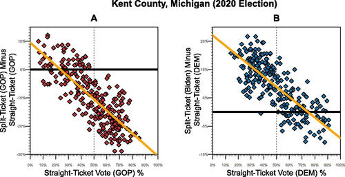
In the United States, the voting experience varies widely. Some jurisdictions offer a ’straight ticket’ option, enabling voters to choose all candidates from one party with a single checkbox. Alternatively, voters can select individual candidates for each office. An observed trend, as noted by Ayyadurai (2020), suggests a correlation between Trump’s voter support in precincts with a high proportion of straight-ticket voting and a decrease in his appeal among split-ticket voters, who select individual candidates from different parties.⁴⁵ He hypothesizes that when support levels between straight and split ticket votes are similar, it points to regular voting behavior; deviations might suggest anomalies like voter fraud. But this premise is wrong.

Ayyadurai’s analysis involves a scatterplot with one axis showing the difference in Trump’s support between non-straight-ticket and straight-ticket voters, and the other axis displaying Trump’s straight-ticket vote percentage. His hypothesis anticipates no correlation, indicating normal voting behavior. This study uses data from four Michigan counties where voters had the option of straight-ticket voting. A negative correlation, according to Ayyadurai, could imply manipulation of split-ticket votes, potentially affecting Trump’s vote share. Ayyadurai’s hypothesis assumes that in the absence of fraud, the relationship’s slope should be zero.

We can write this argument as

If the difference between straight ticket vote share for the candidate of a given party and split ticket vote share for the candidate of that party is negatively correlated with total votes for that candidate (A),

then there is vote fraud in favor of the other party (B).

The difference between straight ticket vote Republican share and split ticket Republican vote share in four Michigan counties is negatively correlated with straight ticket Republican vote share (A).

Therefore, there must have been vote fraud favoring the Democrats in those counties (B).

Although structurally sound, the argument has statistical and logical shortcomings.

Figure 6A replicates Ayyadurai’s plot for Kent County, revealing a noticeable negative correlation. However, this correlation does not indicate fraud. It reveals that in precincts with higher straight-ticket voting for a party, fewer split-ticket voters choose Trump. Figure 6B, mirroring Ayyadurai’s approach but from a Democratic perspective, also shows a negative correlation. Since fraud cannot disfavoring both candidates, this pattern is not about fraud at all. Indeed, the negative correlation Ayyadurai highlights is expected anytime the proportion of split-ticket votes for a candidate is less than the party’s straight-ticket vote share. And, in 2020, both Trump and Biden received fewer votes among split ticket voters when compared to those who voted straight ticket. Thus, the key question is not the negative correlation itself but why Trump (or Biden) secures a lower split-ticket vote share relative to their straight-ticket share. This trend can be explained by conditional probability, not fraud.⁴⁶

Fig. 6 Kent County, Michigan 2020 election data plotted as Ayyadurai shows it.

NOTE: Plot A shows the same data and scatterplot showing Ayyadurai’s YouTube video. Plot B shows the pattern when using Biden’s share of the vote plotted in the same manner. Each point is a precinct in Kent County, Michigan, one of the four counties analyzed in Ayyadurai’s video. 252 total precincts. The slope of the regression line in plot A is–0.40 and plot B is–0.36.

Data: https://electionreporting.com/4539283c-3f09-4fdf-ad93-0bfd82d32be1/county/db3f9865-656b-4704-9429-bd38e726ab42

We observe two types of split-ticket voters: those who vote for Trump and at least one Democrat for another office and those who choose Biden and at least one Republican for another offices. We expected a strong positive correlation between the candidate’s straight-ticket and split-ticket vote in precincts (Figure 7). But we should not expect a perfect correlation. Take for instance a precinct where among the straight ticket vote, 100% are choosing Trump. Unless the split ticket voters are all choosing Trump and voting Democrat down ticket, the percent for Trump among this set of voters will be less than 100%. Thus, in Ayyadurai’s plots, one would find a negative correlation! Ayyadurai also notes that Trump’s vote share among split-ticket voters is higher in precincts with predominantly Democratic straight-ticket votes. This is for exactly the same reason; when Biden is receiving 100% of the straight-ticket votes, its only possible for him to receive less than 100% of the split-ticket vote!

Fig. 7 Kent county, Michigan precinct comparison between Trump straight-ticket and Trump split-ticket support.

NOTE: Each point is a precinct in Kent County, Michigan, one of the four counties analyzed in Ayyadurai’s video. 252 total precincts. The slope of the regression line in plot A is 0.60 and plot B is 0.64.

Data: https://electionreporting.com/4539283c-3f09-4fdf-ad93-0bfd82d32be1/county/db3f9865-656b-4704-9429-bd38e726ab42

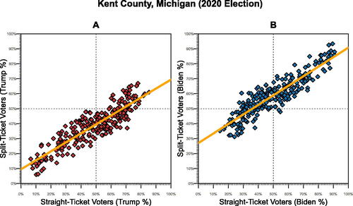
In sum, in heavily Republican precincts (via straight-ticket, since all straight-ticket voters are choosing Trump), split-ticket voters tend to vote against Trump, and vice versa in Democratic precincts. Therefore, a precinct’s dominant party affiliation can influence the direction of split-ticket voting. This phenomenon, rooted in politics and conditional probabilities, can result in the negative correlation seen in Ayyadurai’s data.

2.6.2 Comparison of Differences Involving Samples with Different Means

There’s a second type of fallacy involved with the examples shown in Ayyadurai. It is claimed that in Wayne County the pattern is different than the other four counties (no correlation), and therefore the algorithm that transferred votes to Biden was not used. However, one need only look at the x-axis to see that in Wayne County the most Republican precinct has only about 30% Trump support.⁴⁷ In the other counties, some precincts have 80% Trump support. In the range of the Wayne County plot, the pattern is like the other counties. One must be careful when presenting or consuming information from graphs that may mislead, even if done in ways that are not intentional. In this case, the data simply does not exist such that there are heavily Republican precincts in Wayne County to compare to the other counties.

2.6.3 Matching Design (within-Election Comparisons of Areas with and without Fraud Claims)

Lott (2020) offers various apparently sophisticated attempts to prove election fraud via statistical analysis.⁴⁸ One analysis looks at what are intended to be matched (adjacent) pairs of units in different states with one of the two in a county having allegations of vote fraud and the other not, with a further comparison to differences between adjacent units in areas where there was no allegation of fraud. The differences he examines are dissimilarities between pairs of units in the share of the Trump vote that comes from ballots that were cast in-person versus those that were cast in the form of absentee ballots. This is a difference-in-differences analysis. The basic claims are that such differences between otherwise matched units can provide evidence bearing on whether fraud claims are genuine.

The research design for such a claim appears to be plausible on its face, but the matching was flawed. As Eggers, Garro, and Grimmer (2021, pp. 24–26) point out, in matching units in adjacent counties where Trump won, it is arbitrary which unit we list first, and they show that reversing the order overturns the conclusion that there was fraud benefiting Biden. Second, they show that when one runs a more straightforward statistical test on the same data, the conclusions about fraud again fail to be supported.

Moreover, differences in Trump share of in-person and not in-person votes can be expected to vary with the size of the Trump vote in the unit, since Trump strongly discouraged voting absentee or by mail. Thus, the more Trump supporters in the unit, the more likely it is that Trump’s support will be higher among the in-person voters than among those who do not vote in-person. This fact makes it absurd to conclude that the differences between in-person and not in-person voting that Lott found demonstrate fraud, since the units being compared differ in their vote for Trump and thus can be expected to differ in the relative levels of in-person and not in-person support for Mr. Trump.

The second test Lott (2020) runs involves national data on units within battleground states. The claim is that, controlling for relevant factors, turnout in units where fraud was alleged are marginally higher than turnout predicted by a set of covariates. One key problem is that, as Eggers, Garro, and Grimmer (2021, pp. 31–38) show, this claim does not survive reanalysis of the data. They show that we would get the same conclusions of fraud if we randomly chose counties from the set of states Lott examines, since the purported fraud differences can be linked to state-wide differences in change in turnout. A more basic problem is that small turnout differences on the order of magnitude of those found in Lott (2020) are not in any way direct evidence of fraud, since there are factors not controlled for, such as mobilization efforts.

3 Conclusions

To paraphrase Jeremy Bentham, claims of massive fraud based on aggregate level statistical features of the 2020 election are not just nonsense, but “nonsense on stilts” (Bentham, 2002). While it is impossible to address all the misleading claims and specious arguments made on the internet or even by President Trump himself, we believe the compendium of statistical fallacies given above can be useful to those interested in the misuse of statistics. And, as noted earlier, this essay is deliberately written in a nontechnical way to be comprehensible to beginning students in statistics. We anticipate that this essay will serve journalists and educators in several key ways: first, by presenting targeted rebuttals to current assertions, and offering easily accessible corrections; second, by clarifying different statistical fallacies, aiding in the identification and indexing of claims that use scientific terminology yet lack theoretical or statistical robustness; and third, by delivering original data analysis that counters claims of widespread fraud in the 2020 election.

There are many reasons that can be offered about why beliefs about massive election fraud in 2020 persist (see e.g., Douglas et al., 2019; Holman and Lay, 2019; Berlinski et al., 2021; Edsall, 2022). While explaining why these repeated lies about the 2020 election having been stolen have been believed by so many voters is not the topic of this essay, there are a few points made by others that bear repetition.

One obvious key factor is the level of present-day polarization, in which partisan identities shape beliefs (Abramowitz and Webster, 2018; Iyengar et al., 2019). Strongly embedded partisan identities mean that the public polarizes on the fraud claim based on partisanship. Relatedly, Lenz (2012), among others, has shown that the public changes its policy views to match the politicians they support (e.g., attitudes toward Russia among Republicans track Trump’s changing views about Putin). The fraud claims are echoed as indisputable by a multiplicity of sources that some voters trust (see above about Dominion and Fox News). Also, sources supporting the claim of Trump’s having won the 2020 election denigrate the reliability of the mainstream media which refute the fraud claim and insist that the mainstream media are simply partisan mouthpieces for the Democrats. Relatedly, we have a siloization of communication channels along partisan and ideological lines (Prior, 2013; Robertson et al., 2023). When attitudes are polarized, the importance of siloization of voter information patterns as an explanation for voter beliefs may, however, be overemphasized.

In this essay, our focus has largely been on countering assertions made by Republicans. However, it’s important to note that the misuse of statistics transcends partisanship. Indeed, individuals from all political affiliations can and do fall prey to statistical errors. Our emphasis on former President Trump and his associates stems from the extensive nature and repeated circulation of their claims, despite substantial counterarguments. This pattern suggests either a remarkable level of credulity or a concerted effort to mislead. Given the significant harm caused by these falsehoods, we stress the importance of ongoing efforts to combat misinformation.

Supplementary Materials

Supplementary material includes all data and replication code needed to reproduce tables, figures, and statistical analyses in this paper. Supplementary materials for this article are available online. Please go to www.tandfonline.com/r/JSPP.

Acknowledgments

This research received partial support from the Peltason Chair of Democracy Studies at the University of California, Irvine. The opinions presented are exclusively those of the authors. We extend our gratitude to Sean Birch for his invaluable assistance, and to Dan Silverman and John Chin for their meticulous line-by-line revisions. Our thanks also go to the reviewers and editor for their constructive suggestions. The article benefited significantly from insights gained at the Carnegie Mellon Institute for Strategy & Technology’s Political Science Research Workshop. Additionally, the European Political Science Association panel, especially discussant Jeff Gill, provided crucial feedback.

Disclosure Statement

No potential conflict of interest was reported by the author(s).

Notes

1 For example, see Figure 3. Donald Trump has a history of making claims about fraud in elections. After the 2016 election in which he was victorious, he claimed that millions of non-citizens voted, preventing him from winning the popular vote. Those claims were also false (Cottrell, Herron, and Westwood, 2018). Before that, Trump promoted the claim that President Obama was not born in the United States, and thus not eligible to be president (Reeve, 2012; Jardina and Traugott 2019). This, too, is a false claim.

2 Evidence suggests that these voters sincerely hold these beliefs (Cuthbert and Theodoridis, 2022; Fahey, 2023. See Peterson and Iyengar, 2021).

3 Over 170 federal or statewide candidates who denied the legitimacy of the 2020 U.S. presidential election won their general election contests in November 2022. Thus, although many of the over 291 election denying candidates for these offices that emerged from the primary lost in the general election, some won their elections, and some can exert direct or indirect influence on future election administration. See for example Blanco, Wolfe, and Gardner (2022).

4 Nearly three in 10 Americans reacted positively to the statement “If elected leaders will not protect America, the people must do it themselves even if it requires taking violent actions” (Cox, 2021).

5 “Of the 64 cases brought by Trump and his supporters, twenty were dismissed before a hearing on the merits, fourteen were voluntarily dismissed by Trump and his supporters before a hearing on the merits, and 30 cases included a hearing on the merits. Only in one Pennsylvania case involving far too few votes to overturn the results did Trump and his supporters prevail (Danforth et al., 2022; p. 3).

6 Former President Trump and some of his supporters are now indicted in two cases, one if federal court, one in state court. The first of these cases is in federal court in Washington D.C. and includes four counts. Prosecutors argue that the claims made by Trump “were false, and [Trump] the defendant knew that they were false” (Indictment, p. 7). They also charge that he “deliberatively disregarded the truth.” A second case is in state court in Georgia (Sullivan, Ax, and Lynch, 2023). The indictment details various alleged offenses by Trump and his associates, encompassing giving false testimony to legislators about election fraud and pressuring state officials to breach their official duties by nullifying the election outcomes.

7 In April of 2023, Dominion, a company who manufactures voting machines, reached a settlement of $787.5 million in a defamation lawsuit again Fox News for the propagation of claims that Dominion machines changed votes from Trump to Biden (Poniewozik, 2023). To prove defamation, one must show “’actual malice’–that the statement was made with knowledge of its falsity or with reckless disregard of whether it was true or false.” New York Times v. Sullivan 376 U.S. 254 (1964). In documents that were revealed during the discovery phase of the trial, Fox News host admitted that they did not believe the claims they were making on television but repeated them because “[o]ur viewers are good people and they believe it” (Poniewozik, 2023).

8 We hold the view that statements supported by statistical evidence can be especially pernicious. This is demonstrated by how challenging established scientific consensus can sway public opinion, as indicated in the study by Lewandowsky, Gignac, and Vaughan (2013).

9 Describing the Russian model of propaganda, RAND has coined the phrase “firehose of falsehood.” It is called this because of the distinctive pattern of a “high numbers of channels and messages and a shameless willingness to disseminate partial truths or outright fictions” (Paul and Matthews, 2016). We prefer to think of them as a hydra-headed monster, for every piece of misinformation corrected, multiple new ones are created (“Since the Hydra could replace old heads with multiple new ones…logic requires that the creature boasted different numbers of heads at different times.” Ogden, 2013).

10 We would also note that, in the four years before the election, the claim that the 2020 election would be stolen by the Democrats was also repeatedly asserted by President Trump and his supporters, thus preparing the way for the post-election claims of fraud.

11 See, for example, Bump (2022). We will, however, make a few points about misperceptions and misinformation in the concluding section of this article.

12 We do, however, believe that the framework of classifying election-related statistical fallacies that we offer may prove useful to other scholars.

13 We would call particular attention to the excellent survey and analysis of 2020 presidential election fallacies by Eggers, Garro, and Grimmer (2021). We began writing our own essay before we were familiar with this article in its on-line form, but we have learned a lot from it and cite to it herein. Their detailed rebuttal of fallacies is more technical than ours, and we cover some fallacies that they do not. There are also various journalistic surveys of election fraud claims (Corasaniti, Epstein, and Rutenberg, 2020; Feldman, 2020; Alba and Frenkel, 2021), but these primarily include claims that do not fall within the scope of this essay.

14 Moreover, in understanding Electoral College outcomes, we need also to look at the geographic location of each candidate’s support. See Box 2.

15 As of 2020, there were 3143 total counties and county equivalents. In our data, we have 3153 because Alaska reports election results from Electoral Districts, of which there were 10 more than their county equivalents.

16 Data is estimated, as no official national election results are compiled. Dave Leip’s Atlas of Presidential Elections, a well-reputed compiler of election results, reports totals that do not match the certified, official federal elections results produced by the FEC. The Brookings Institute reports the differential to be 2588 Trump counties to 551 Biden counties (Frey, 2021).

17 The number of votes cast in Los Angeles County surpassed the total votes in 39 states!

18 For a nice overview of political graphics of different kinds, including a cartogram of the 2020 presidential election at the county level, see Bliss and Patino (2020). See also Cartographic Views of the 2020 US Presidential Election - Worldmapper (2020).

19 The bubble size gradations on a bubble map make this task easier than the color variations on a cartogram that usually have a limited number of victory margin categories. Though, note that the circle size in our map is scaled using the square root of the vote total, so the circle size itself is not a linear scale.

20 https://plato.stanford.edu/entries/paradox-simpson//#:∼:text=Simpson’s%20Paradox%20is%20a%20statistical,population%20is%20divided%20into%20subpopulations.

21 Top row is the proportion of the electorate for each demographic group.

22 Academics and journalists, including ourselves, often limit our analysis of election results to the two major parties. To do so, we convert results into the two-party vote share and eliminate all non-major party candidates. But, doing so can shield important insights, such as those highlighted in this section.

23 As we noted earlier, we are providing a compendium; this and other claims of Dr. Cicchetti have already been rebutted elsewhere (see e.g., http://web.archive.org/web/20220416221931/, https://reason.com/volokh/2020/12/09/more-on-statistical-stupidity-at-scotus/, and http://web.archive.org/web/20220416221815/https://statmodeling.stat.columbia.edu/2020/12/08/the-p-value-is-4-76x10%E2%88%92264-1-in-a-quadrillion/. That report has been devastatingly critiqued in the expert witness report of Gary King in the same case. Claims about election fraud in Texas v. Pennsylvania, including Dr. Cicchetti’s report, can be found here: https://www.supremecourt.gov/DocketPDF/22/22O155/163048/20201208132827887_TX-v-State-ExpedMot%202020-12-07%20FINAL.pdf

24 In the hearings by the House Select Committee investigating January 6, this discrepancy between the patterns in early and late votes was referred to as a “red mirage.”

25 Perhaps because states with more Democrats allow for more wide-spread use of mail-in balloting, for example, eight states conduct general elections entirely by mail. They include California, Colorado, Hawaii, Nevada, Oregon, Utah, Vermont, and Washington. See (Voting Outside the Polling Place: Absentee, All-Mail and Other Voting at Home Options, 2022). All of these, except Utah, voted their electors to both Democratic nominees Clinton (2016) and Biden (2020).

26 Two states, Connecticut (Conn. Gen. Stat. §9-150a) and Ohio (Ohio Rev. Code §3509.06), do not specify when counting may begin. For more information, see Voting Outside the Polling Place: Absentee, All-Mail and Other Voting at Home Options (2022; Table 16).

27 This study includes a comparison of the assumption of uniform distribution of year of birth and name distribution to actual data and show that assuming a uniform distribution over a 64-year interval and over the names in the dataset tends to underestimate the prevalence of birth year matching by about $12\%\cong \frac{(487\text{-}433)}{433}$ (see p. 119). The more there are birth bulges (as in the post-WWII baby boom), the more likely it is that two randomly chosen individuals will share the same year of birth, and some names are much more prevalent than others.

28 Moreover, as a further complication, we must consider the degree of heterogeneity in the distribution of names. Calculating this probability from the name distribution in the population requires calculating an average based on name and surname. Names vary greatly in their frequency and vary geographically. The U.S. Bureau of the Census publishes a list of surname frequencies based on national values, but the distribution of names (and their degree of heterogeneity) will vary with the racial/ethnic composition of the political unit (Grofman and Garcia, 2014, 2015).

29 Birth year and name are not fully independent of one another. Changing patterns of immigration affect the relative surname shares in different generations, and some rather dramatic changes over time in the popularity of first names mean that first name probabilities are not independent of the year of birth. Also, first and last names are far from independent since both are linked to ethnicity. Indeed, we could, in principle, estimate birth decade probabilities just by looking at the prevalence of first and last names of those born during the decade (see, Grofman and Garcia, 2014, 2015)

30 Note that the probability of finding such a match from among a set of n voters must not be confused with the probability of any specific name + birthday + birthyear combination being repeated. For obvious reasons, the likelihood of a given combination being repeated will depend, ceteris paribus, on how common is the name. We can further simplify by assuming a uniform distribution across the first two factors and assess the likelihood of two randomly chosen individuals bearing the same name from the name distribution in empirical data.

31 And, of course, this assumes that the probabilities are independent of each other.

32 For further compatibility with the McDonald and Levitt (2008) study, in the model presented below, we also took our birth year time-period as a 64-year span.

33 Mebane (2020) notes that “It is widely understood that the first digits of precinct vote counts are not useful for trying to diagnose election frauds.”

34 Wikipedia entry on Benford’s Law: https://en.wikipedia.org/wiki/Benford%27s/_law/#cite/_note-37

35 See for example, Deckert, Myagkov, and Ordeshook (2011). Even Mebane, who has been a repeated applicant of the Law as a fraud detector in elections in multiple countries, has reiterated that while its violation might be taken as suggesting an anomaly, a violation of the supposed law does not prove fraud. Fraud would need to be directly investigated (Mebane, 2020).

36 In Pennsylvania, this included pointing viewers to a website developed by the Department of State. Ads featured prominent actors and athletes from the state explained how to find a location to cast a ballot or how to cast a ballot by mail.

37 Trump’s White House Press Secretary Kayleigh McEnany falsely claimed that “[a] mere survey of the facts shows that voters in blue counties like Philadelphia County were given certain privileges that voters in red counties were not afforded. The Constitution’s equal protection clause requires uniform standards, but Democrat election officials created disparities depending on where citizens lived and where they voted in the state.” However, the PA Department of State gave guidance to all counties that they could allow voters to make corrections to rejected mail-in ballots. Some counties, predominantly Trump-majority in their partisanship, choose not to.

38 See Morris Fiorina (2017) “Unstable Majorities”, and Frances Lee (2016) “Insecure Majorities”. Modern elections are very likely to result in divided government, and control of any branch of government is often won or lost in the margins. Partisan bias, such as that introduced by malapportionment or gerrymandering, can also affect the ability to carry marginal House or Senate seats.

39 For more details on Biden’s overperformance compared to U.S. House Democratic candidates, see William A. Galston (2020).

40 House Democrats nationally underperformed their 2018 performance, which accounts for the fourteen net seats gained by the Republicans. Relative to the 115th Congress (2016–2018), the 177th Congress (2021–2023) has 28 more Democrats.

41 Figure omitted for space reasons.

42 An increase of 22 from 2016.

43 A decrease by 19 from 2016.

44 This “thread” is filled with statistics purportedly showing how Biden is the historic underdog going into the 2020 election (by this account, Trump should have been heavily favored), for example, “Incumbents are 6/6 when facing re-election during civil unrest”. See more: https://twitter.com/davidchapman141/status/1315440579485069314?s=20 Internal links to this claim on Twitter say that the first primary was in 1912 and that Trump had received a higher percentage of the primary vote than Eisenhower, Nixon, Clinton, and Obama. And it is noted that only five incumbents have received at least 90% of their primary vote.

45 He unnecessarily complicates this by plotting on the y-axis the difference between the split-ticket vote and the straight-ticket vote, as explained in the following paragraphs.

46 This rebuttal to Ayyadurai (2020) is presented in Eggers, Garro, and Grimmer (2021), acknowledging its previous elucidation by Kabir (2020) and Parker (2020), each of whom show empirical evidence of the party-independence of results. However, the Eggers, Garro, and Grimmer main rebuttal to the Ayyadurai (2020) claim uses the logic of latent variable analysis by demonstrating how regression to the mean effects lead to negatively sloped regression lines in the situation posited by Ayyadurai.

47 Not shown due to space constraints. Can be seen at the 39 min mark in his original video.

48 For more information about Lott’s research in his own words, see a blog post he wrote himself at RealClear Politics, titled “New Peer-Reviewed Research Finds Evidence of 2020 Voter Fraud.” (Lott, 2020). To the best of our knowledge, this research has not yet been published in a peer-reviewed journal.

References

- Abramowitz, A. I., and Webster, S. W. (2018), “Negative Partisanship: Why Americans Dislike Parties but Behave like Rabid Partisans: Negative Partisanship and Rabid Partisans,” Political Psychology, 39, 119–135. DOI: 10.1111/pops.12479.
- Alba, D., and Frenkel, S. (2021), “Watch Out for This Misinformation When Congress Meets to Certify the Election.” The New York Times. Available at https://www.nytimes.com/2021/01/06/business/election-fraud.html (Accessed November 25, 2023).
- Ayyadurai, S. (2020), “Dr.SHIVA LIVE: MIT PhD Analysis of Michigan Votes Reveals Unfortunate Truth of U.S. Voting Systems,” November 10. Available at https://www.youtube.com/watch?v=Ztu5Y5obWPk
- Bentham, J. (2002), “Rights, Representation, and Reform: Nonsense upon Stilts and Other Writings on the French Revolution,” in The Collected Works of Jeremy Bentham (1st ed.), eds. P. Schofield, C. Pease-Watkin, and C. Blamires, pp. 317–401, Oxford: Oxford University Press.
- Berlinski, N., Doyle, M., Guess, A. M., Levy, G., Lyons, B., Montgomery, J. M., Nyhan, B., and Reifler, J. (2021), “The Effects of Unsubstantiated Claims of Voter Fraud on Confidence in Elections,” Journal of Experimental Political Science, 10, 34–49. DOI: 10.1017/XPS.2021.18.
- Better Know a Ballot. (2021), “A Late Show with Stephen Colbert,” Available at https://www.betterknowaballot.com/
- Bishop, B., and Cushing, R. G. (2008), The Big Sort: Why the Clustering of Like-minded America is Tearing Us Apart, New York: Houghton Mifflin. https://books.google.com/books?id=NXN2AAAAMAAJ.
- Blanco, A., Wolfe, D., and Gardner, A. (2022), “Tracking which 2020 Election Deniers are Winning, Losing in the Midterms.” Washington Post. Available at https://www.washingtonpost.com/politics/interactive/2022/election-deniers-midterms/
- Bliss, L., and Patino, M. (2020), “How to Spot Misleading Election Maps,” Bloomberg CityLab. Available at https://www.bloomberg.com/news/articles/2020-11-03/a-complete-guide-to-misleading-election-maps
- Bump, P. (2022), “We have Reached the Apex of Election-Fraud Debunking,” The Washington Post, July 14. Available at https://www.washingtonpost.com/politics/2022/07/14/we-have-reached-apex-election-fraud-debunking/
- Campbell, J. E. (1986), “Presidential Coattails and Midterm Losses in State Legislative Elections,” American Political Science Review, 80, 45–63. DOI: 10.2307/1957083.
- Cartographic Views of the 2020 US Presidential Election - Worldmapper (2020), World Mapper November 27. Available at https://worldmapper.org/us-presidential-election-2020/
- Cervas, J. R., and Grofman, B. (2019), “Are Presidential Inversions Inevitable? Comparing Eight Counterfactual Rules for Electing the U.S. President*,” Social Science Quarterly, 100, 1322–1342. DOI: 10.1111/ssqu.12634.
- Corasaniti, N., Epstein, L., and Rutenberg, J. (2020), “Election Officials Nationwide Find No Fraud,” The New York Times, A1, November 11, Available at https://www.nytimes.com/2020/11/10/us/politics/voting-fraud.html
- Cottrell, D., Herron, M. C., and Westwood, S. J. (2018), “An Exploration of Donald Trump’s Allegations of Massive Voter Fraud in the 2016 General Election,” Electoral Studies, 51, 123–142. https://www.sciencedirect.com/science/article/pii/S026137941730166X DOI: 10.1016/j.electstud.2017.09.002.
- Cox, D. A. (2021), “After the Ballots are Counted: Conspiracies, Political Violence, and American Exceptionalism.” The Survey Center on American Life. https://www.americansurveycenter.org/research/after-the-ballots-are-counted-conspiracies-political-violence-and-american-exceptionalism/
- Cuthbert, L., and Theodoridis, A. (2022), “Do Republicans really believe Trump won the 2020 election? Our Research Suggests that they do.” Washington Post. Available at https://www.washingtonpost.com/politics/2022/01/07/republicans-big-lie-trump/
- Danforth, J., et al. (2022), “Lost, Not Stolen: The Conservative Case that Trump Lost and Biden Won the 2020 Presidential Election,” Available at https://lostnotstolen.org
- Deckert, J., Myagkov, M., and Ordeshook, P. C. (2011), “Benford’s Law and the Detection of Election Fraud,” Political Analysis, 19, 245–268. https://www.cambridge.org/core/journals/political-analysis/article/benfords-law-and-the-detection-of-election-fraud/3B1D64E822371C461AF3C61CE91AAF6D (Accessed November 25, 2023).
- Deutsch, K. W., and Madow, W. G. (1961), “A Note on the Appearance of Wisdom in Large Bureaucratic Organizations,” Behavioral Science, 6, 72–78. DOI: 10.1002/bs.3830060108.
- “DNC Launches New Digital Ads in PA Reaching Vote-By-Mail Voters: ‘How To Return Your Ballot!”’ (2020), Democratic National Committee. Available at https://democrats.org/news/dnc-launches-new-digital-ads-in-pa-reaching-vote-by-mail-voters-how-to-return-your-ballot/ (Accessed November 25, 2023).
- Douglas, K. M., Uscinski, J. E., Sutton, R. M., Cichocka, A., Nefes, T., Ang, C. S., and Deravi, F. (2019), “Understanding Conspiracy Theories,” Political Psychology, 40, 3–35. DOI: 10.1111/pops.12568.
- Downs, A. (1957), An Economic Theory of Democracy. New York: Harper & Row.
- Edlin, R., and Norden, L. (2023), “Poll of Election Officials Shows High Turnover Amid Safety Threats and Political Interference.” Brennan Center for Justice. Available at https://www.brennancenter.org/our-work/analysis-opinion/poll-election-officials-shows-high-turnover-amid-safety-threats-and
- Edsall, T. B. (2022), “Why Conspiracy Theories Flourish in Trump’s America,” The New York Times, June 22. Available at https://www.nytimes.com/2022/06/22/opinion/trump-conspiracy-theories.html
- Eggers, A. C., Garro, H., and Grimmer, J. (2021), “No Evidence for Systematic Voter Fraud: A Guide to Statistical Claims about the 2020 Election,” Proceedings of the National Academy of Sciences, 118, e2103619118. DOI: 10.1073/pnas.2103619118.
- Engstrom, E. J. (2020), “Congressional Elections: Electoral Structure and Political Representation,” in New Directions in American Politics, eds. J. L. Carson and M. S. Lynch, pp. 9–29, New York: Taylor & Francis. https://books.google.com/books?id=-CnZDwAAQBAJ
- Fahey, J. J. (2023), “The Big Lie: Expressive Responding and Misperceptions in the United States,” Journal of Experimental Political Science, 10, 267–278. https://www.cambridge.org/core/journals/journal-of-experimental-political-science/article/big-lie-expressive-responding-and-misperceptions-in-the-united-states/BCD84FDE078F10B9E87335A061EBDE85
- Farley, R. (2020), “Ballot “Curing” in Pennsylvania - FactCheck.org,” FactCheck.Org, November 13. Available at https://www.factcheck.org/2020/11/ballot-curing-in-pennsylvania/
- Feldman, M. (2020), “10 Voter Fraud Lies Debunked,” Available at https://www.brennancenter.org/our-work/research-reports/10-voter-fraud-lies-debunked
- Fiorina, M. P. (2017), Unstable Majorities. Stanford, CA: Hoover Institution Press.
- Foley, E. B., and Stewart Iii, C. (2020), “Explaining the Blue Shift in Election Canvassing,” Journal of Political Institutions and Political Economy, 1, 239–265. https://www.nowpublishers.com/article/Details/PIP-0010 (Accessed November 25, 2023). DOI: 10.1561/113.00000010.
- Frey, W. H. (2021), “Biden-Won Counties are Home to 67 Million More Americans than Trump-Won Counties,” Brookings, January 21. Available at https://www.brookings.edu/blog/the-avenue/2021/01/21/a-demographic-contrast-biden-won-551-counties-home-to-67-million-more-americans-than-trumps-2588-counties/
- Galston, W. A. (2020), “Why Did House Democrats Underperform Compared to Joe Biden?” Brookings, December 21. Available at https://www.brookings.edu/blog/fixgov/2020/12/21/why-did-house-democrats-underperform-compared-to-joe-biden/.
- Gardner, A. (2021), “In Ramp-Up to 2022 Midterms, Republican Candidates Center Pitches on Trump’s False Election Claims - The Washington Post,” The Washington Post, July 5. Available at https://www.washingtonpost.com/politics/republican-trump-2022-midterms-election-falsehoods/2021/07/04/3a43438c-d36f-11eb-ae54-515e2f63d37d/_story.html
- Gelman, A. (2021), August 21). Alex Jones and the fallacy of the one-sided bet. Statistical Modeling, Causal Inference, and Social Science. Available at https://statmodeling.stat.columbia.edu/2021/08/21/alex-jones-and-the-fallacy-of-the-one-sided-bet/
- Gray, J. (2020), “Georgia Election Officials Show Frame-by-Frame What Happened in Fulton Surveillance Video–WSB-TV Channel 2–Atlanta,” WSB-TV 2 Atlanta, December 4. Available at https://www.wsbtv.com/news/politics/georgia-election-officials-show-frame-by-frame-what-really-happened-fulton-surveillance-video/T5M3PYIBYFHFFOD3CIB2ULDVDE/
- Grofman, B. (2022), “Prospects for Democratic Breakdown in the United States: Bringing the States Back In,” Perspectives on Politics, 20, 1040–1047. DOI: 10.1017/S1537592721003285.
- Grofman, B., and Chen, H. (2022), “Understanding the Factors That Affect the Incidence of Bellwether Counties: A Conditional Probability Model,” Political Research Quarterly, 76, 119–126. DOI: 10.1177/10659129211057601.
- Grofman, B., and Garcia, J. R. (2014), “Using Spanish Surname to Estimate Hispanic Voting Population in Voting Rights Litigation: A Model of Context Effects Using Bayes’ Theorem,” Election Law Journal: Rules, Politics, and Policy, 13, 375–393. DOI: 10.1089/elj.2013.0190.
- Grofman, B., and Garcia, J. R. (2015), “Using Spanish Surname Ratios to Estimate Proportion Hispanic in California Cities via Bayes Theorem*,” Social Science Quarterly, 96, 1511–1527. DOI: 10.1111/ssqu.12214.
- Hasen, R. L. (2020), Election Meltdown: Dirty Tricks, Distrust, and the Threat to American Democracy, New Haven, CT: Yale University Press. https://www.amazon.com/Election-Meltdown-Distrust-American-Democracy/dp/0300248199
- Holman, M. R., and Lay, J. C. (2019), “They See Dead People (Voting): Correcting Misperceptions about Voter Fraud in the 2016 U.S. Presidential Election,” Journal of Political Marketing, 18, 31–68. (Accessed November 25, 2023). DOI: 10.1080/15377857.2018.1478656.
- Homans, C., and Peterson, M. (2022), “How ‘Stop the Steal’ Captured the American Right,” The New York Times, July 24. Available at https://www.nytimes.com/2022/07/19/magazine/stop-the-steal.html
- Hopkins, D. A. (2017), Red Fighting Blue, Cambridge: Cambridge University Press. DOI: 10.1017/9781108123594.
- Hsu, T., and Thompson, S. A. (2022), “Hunting for Voter Fraud, Conspiracy Theorists Organize ‘Stakeouts’,” The New York Times, August 10. Available at https://www.nytimes.com/2022/08/10/technology/voter-drop-box-conspiracy-theory.html
- Iyengar, S., Lelkes, Y., Levendusky, M., Malhotra, N., and Westwood, S. J. (2019), “The Origins and Consequences of Affective Polarization in the United States,” Annual Review of Political Science, 22, 129–146. DOI: 10.1146/annurev-polisci-051117-073034.
- Jacobson, G. C. (2019), “Extreme Referendum: Donald Trump and the 2018 Midterm Elections,” Political Science Quarterly, 134, 9–38. DOI: 10.1002/polq.12866.
- Jacobson, G. C. (2023), “The Dimensions, Origins, and Consequences of Belief in Donald Trump’s Big Lie,” Political Science Quarterly, 138, 133–166. DOI: 10.1093/psquar/qqac030.
- Jardina, A., and Traugott, M. (2019), “The Genesis of the Birther Rumor: Partisanship, Racial Attitudes, and Political Knowledge,” The Journal of Race, Ethnicity, and Politics, 4, 60–80. https://www.cambridge.org/core/journals/journal-of-race-ethnicity-and-politics/article/genesis-of-the-birther-rumor-partisanship-racial-attitudes-and-political-knowledge/8C13EDF7D45A475E97B5D2B35BC8979E/#
- Jenny. (2020), November 7), “Joe Biden’s votes violate Benford’s Law. 0–1,” November 7. Available at https://web.archive.org/web/20220417144342/https://gnews.org/534248/
- Kabir, N. (2020), “The Fraud Of Dr. Shiva Ayyadurai: Oakland County, Michigan |by Naim Kabir |Medium,” Medium, November 14. Available at https://naim-kabir.medium.com/the-fraud-of-dr-shiva-ayyadurai-oakland-county-michigan-1bc51bcebf1b
- Kessler, G. (2020), “The Biggest Pinocchios of 2020,” The Washington Post, December 18. Available at https://www.washingtonpost.com/politics/2020/12/18/biggest-pinocchios-2020
- Lai, J. (2020), “How ‘Naked Ballots’ in Pennsylvania Could Cost Joe Biden the Election,” The Philadelphia Inquirer, September 21.
- Lee, F. E. (2016), Insecure Majorities: Congress and the Perpetual Campaign. Chicago, IL: University of Chicago Press.
- Lenz, G. S. (2012), Follow the Leader? How Voters Respond to Politicians’ Policies and Performance. Chicago, IL: University of Chicago Press. Available at https://press.uchicago.edu/ucp/books/book/chicago/F/bo11644533.html
- Leonhardt, D. (2022), “Bigger than Trump: Election Conspiracy Theories Have Become Central to the Republican Party,” The New York Times, July 19. Available at https://www.nytimes.com/2022/07/19/briefing/stop-the-steal-anti-democracy.html
- Lewandowsky, S., Gignac, G. E., and Vaughan, S. (2013), “The Pivotal Role of Perceived Scientific Consensus in Acceptance of Science,” Nature Climate Change, 3, 399–404. https://www.nature.com/articles/nclimate1720 DOI: 10.1038/nclimate1720.
- Lipsitz, K. (2011), Competitive Elections and the American Voter, Philadelphia: University of Pennsylvania Press. https://books.google.com/books?id=rJ8s5RFA/_akC.
- Lott, J. R. (2020), “A Simple Test for the Extent of Voter Fraud with Absentee Ballots in the 2020 Presidential Election: Georgia and Pennsylvania Data,” DOI: 10.2139/ssrn.3756988.
- Lott, J. R. (2022), “New Peer-Reviewed Research Finds Evidence of 2020 Voter Fraud.” RealClear Politics. Available at https://www.realclearpolitics.com/articles/2022/03/28/new/_peer-reviewed/_research/_finds/_evidence/_of/_2020/_voter/_fraud/_147378.html
- Matsumoto, R. (2021), “Where Did All The Bellwether Counties Go?” FiveThirtyEight, February 1. Available at https://fivethirtyeight.com/features/where-did-all-the-bellwether-counties-go/
- McClallen, S. (2021), “Over 7,000 Affidavits Delivered to Michigan Lawmakers Claim Election Fraud |Michigan |thecentersquare.com,” The Center Square, June 17. Available at https://www.thecentersquare.com/michigan/over-7-000-affidavits-delivered-to-michigan-lawmakers-claim-election-fraud/article/_78b6812c-cf98-11eb-868e-734c5e3a51de.html
- McDade, A. (2022), “Ohio Secretary of State Touts Security of Election Process After Referring 27 Fraud Cases,” Newsweek, February 1. Available at https://www.newsweek.com/ohio-secretary-state-touts-security-election-process-after-referring-27-fraud-cases-1675215
- McDonald, M. P., and Levitt, J. (2008), “Seeing Double Voting: An Extension of the Birthday Problem,” Election Law Journal: Rules, Politics, and Policy, 7, 111–122. DOI: 10.1089/elj.2008.7202.
- Mebane, W. R. (2011), “Comment on “Benford’s Law and the Detection of Election Fraud,” Political Analysis, 19, 269–272. DOI: 10.1093/pan/mpr024.
- Mebane, W. R. (2020), Inappropriate Applications of Benford’s Law Regularities to Some Data from the 2020 Presidential Election in the United States *. 1045. Available at https://github.com/cjph8914/2020/_benfords
- Mebane, W. R., and Kalinin, K. (2009), Comparative Election Fraud Detection. APSA 2009 Toronto Meeting Paper, 1045. Available at https://papers.ssrn.com/Sol3/papers.cfm?abstract/_id=1450078
- Medina, J., Epstein, R. J., and Corasaniti, N. (2022), “In 4 Swing States, G.O.P. Election Deniers Could Oversee Voting,” The New York Times, August 4. Available at https://www.nytimes.com/2022/08/03/us/politics/gop-election-deniers-trump-arizona-michigan.html
- National Conference of State Legislatures (NCSL). (2022), “Voting Outside the Polling Place: Absentee, All-Mail and Other Voting at Home Options.” National Conference of State Legislatures. Available at https://www.ncsl.org/elections-and-campaigns/voting-outside-the-polling-place (Updated July 12, 2022).
- Norris, P. (2023), “Big Little Election Lies: Cynical and Credulous Evaluations of Electoral Fraud,” Parliamentary Affairs. Available at DOI: 10.1093/pa/gsad022.
- Ogden, D. (2013), Drakon: Dragon Myth and Serpent Cult in the Greek and Roman Worlds, Oxford: Oxford University Press.
- Parker, M. (2020), “Do These Scatter Plots Reveal Fraudulent Vote-Switching in Michigan?” YouTube, November 14. Available at https://www.youtube.com/watch?v=aokNwKx7gM8
- Paul, C., and Matthews, M. (2016), 16 The Russian “Firehose of Falsehood” Propaganda Model Why It Might Work and Options to Counter It, RAND Corporation. Available at https://www.rand.org/pubs/perspectives/PE198.html (Accessed October 30, 2023).
- Pennycook, G., Cannon, T. D., and Rand, D. G. (2018), “Prior Exposure Increases Perceived Accuracy of Fake News,” Journal of Experimental Psychology. General, 147, 1865–1880. DOI: 10.1037/xge0000465.
- Peterson, E., and Iyengar, S. (2021), “Partisan Gaps in Political Information and Information-Seeking Behavior: Motivated Reasoning or Cheerleading?,” American Journal of Political Science, 65, 133–147. https://www.jstor.org/stable/45415617 DOI: 10.1111/ajps.12535.
- Poniewozik, J. (2023), “Everybody Knows What Fox News Is Now.” The New York Times. Available at https://www.nytimes.com/2023/04/19/arts/television/fox-news-settlement.html (Accessed May 24, 2023).
- Prior, M. (2013), “Media and Political Polarization,” Annual Review of Political Science, 16, 101–127. (Accessed October 18, 2022). DOI: 10.1146/annurev-polisci-100711-135242.
- Reality Check team. (2020), “US Election 2020: Fact-checking Trump Team’s Main Fraud Claims - BBC News,” BBC News, November 23. Available at https://www.bbc.com/news/election-us-2020-55016029
- Reeve, E. (2012), “A Case Study in the Evolution of Birtherism: Donald Trump.” The Atlantic. Available at https://www.theatlantic.com/politics/archive/2012/05/slow-evolution-birther-donald-trump-case-study/327629/
- Robertson, R. E., Green, J., Ruck, D. J., Ognyanova, K., Wilson, C., and Lazer, D. (2023), “Users Choose to Engage with More Partisan News than They Are Exposed to on Google Search,” Nature, 618, 342–348. https://www.nature.com/articles/s41586-023-06078-5 (Accessed May 24, 2023). DOI: 10.1038/s41586-023-06078-5.
- Russian elections once again had a suspiciously neat result. (2021), The Economist, October 11. Available at https://www.economist.com/graphic-detail/2021/10/11/russian-elections-once-again-had-a-suspiciously-neat-result
- Sadeghi, M. (2020), “Fact Check: No Evidence Vote Was Cast in Joe Frazier’s Name,” USA Today, November 14. Available at https://www.usatoday.com/story/news/factcheck/2020/11/14/fact-check-no-evidence-late-joe-frazier-voted-2020-election/6283956002/
- Sganga, N. (2022), “U.S. Finds No Evidence Flaws in Dominion Voting Machines Were Ever Exploited - CBS News,” CBS News, June 3. Available at https://www.cbsnews.com/news/dominion-voting-machines-2020-election-cisa/
- Shurk, J. B. (2020), “5 More Ways Joe Biden Magically Outperformed Election Norms,” The Federalist, November 23. Available at https://thefederalist.com/2020/11/23/5-more-ways-joe-biden-magically-outperformed-election-norms/
- Solender, A. (2020), “These Are The Republicans Who Have Acknowledged Biden’s Victory,” Forbes, December 10. Available at https://www.forbes.com/sites/andrewsolender/2020/12/10/these-are-the-republicans-who-have-acknowledged-bidens-victory/?sh=7e71eaea417b
- Sullivan, A., Ax, J., and Lynch, S. N. (2023), “Georgia Charges Trump, Former Advisers in 2020 Election Case.” Reuters. Available at https://www.reuters.com/legal/us-state-georgia-appears-set-file-charges-against-donald-trump-court-document-2023-08-14/
- Swenson, A. (2020), “There Were Not More Votes than Voters in Pennsylvania,” AP News, December 29. Available at https://apnews.com/article/fact-checking-afs:Content:9887147615
- Swenson, A. (2021), “Winning More Counties Doesn’t Translate to an Election Win for Trump,” Associated Press, December 21.
- Thompson, B. G., et al. (2022), “Final Report of the Select Committee to Investigate the January 6th Attack on the United States Capitol,” in Washington: 117th Congress Second Session. Available at https://www.govinfo.gov/content/pkg/GPO-J6-REPORT/pdf/GPO-J6-REPORT.pdf.
- Tufte, E. R. (1974), Data Analysis for Politics and Policy, ed. R. A. Dahl, Englewood Cliffs: Prentice-Hall.
- UMass Amherst. (2021), “Presidential Election & Jan 6th Insurrection at the US Capitol,” UMass Amherst, December 28. Available at https://polsci.umass.edu/toplines-and-crosstabs-december-2021-national-poll-presidential-election-jan-6th-insurrection-us
- Vella, V. (2020), “Delaware County Man Charged with Registering Dead Relatives to Vote in Presidential Election,” The Philadelphia Inquirer, December 21. Available at https://www.inquirer.com/news/bruce-bartman-election-fraud-delaware-county-20201221.html
- Vellani, V., Zheng, S., Ercelik, D., and Sharot, T. (2023), “The Illusory Truth Effect Leads to the Spread of Misinformation,” Cognition, 236, 105421. https://www.sciencedirect.com/science/article/pii/S0010027723000550 DOI: 10.1016/j.cognition.2023.105421.
- Waldman, M. (2023), “Mike Johnson Is Now the Most Powerful Election Denier in Washington.” Brennan Center for Justice. Available at https://www.brennancenter.org/our-work/analysis-opinion/mike-johnson-now-most-powerful-election-denier-washington
- Weiser, W. R., Levitt, J., and Munoz, A. (2006), “Making the List: Database Matching and Verification Processes for Voter Registration.” Brennan Center for Justice. Available at https://www.brennancenter.org/our-work/research-reports/making-list-database-matching-and-verification-processes-voter
- Yourish, K., Buchanan, L., and Denise, L. (2021), “The 147 Republicans Who Voted to Overturn Election Results,” The New York Times. Available at https://www.nytimes.com/interactive/2021/01/07/us/elections/electoral-college-biden-objectors.html
- Zorn, E. (2017), “Polls Reveal Sobering Extent of Nation’s Fact Crisis - Chicago Tribune,” Chicago Tribune, January 5. Available at https://www.chicagotribune.com/columns/eric-zorn/ct-polling-ignorance-facts-trump-zorn-perspec-0106-md-20170105-column.html