Two-sided bounds on some output-related quantities in linear stochastically excited vibration systems with application of the differential calculus of norms

Abstract

A linear stochastic vibration model in state-space form, $\dot{x}(t)=Ax(t)+b(t),x(0)=x_0,$ with output equation $x_S(t)=Sx(t)$ is investigated, where A is the system matrix and b(t) is the white noise excitation. The output equation $x_S(t)=Sx(t)$ can be viewed as a transformation of the state vector x(t) that is mapped by the rectangular matrix S into the output vector x(t). It is known that, under certain conditions, the solution x(t) is a random vector that can be completely described by its mean vector, $m_x(t):=m_{x(t)}$, and its covariance matrix, $P_x(t):=P_{x(t)}$. If matrix A is asymptotically stable, then $m_x(t)\to 0(t\to \infty )$ and $P_{x_S}(t)\to P_S(t\to \infty )$, where $P_S$ is a positive (semi-)definite matrix. Similar results will be derived for some output-related quantities. The obtained results are of special interest to applied mathematicians and engineers.

Keywords:

• linear stochastic vibration system excited by white noise with output equation
• output-related mean vector
• output-related covariance matrix
• two-sided bounds
• differential calculus of norms

AMS Subject Classifications:

• 34D05
• 34F05
• 65L05

Public Interest Statement

When a dynamical system with solution vector x of length n describes an engineering problem, only a few components of x are needed, as a rule. But, nevertheless, the whole pertinent initial value problem must be solved. In order to obtain only the components of interest, one defines an output matrix, say S, that selects them from x by defining the new output vector $x_S:=Sx$ showing its importance. This equation is called output equation. For example, if the engineer wants to apply only the first, second, and nth component, then one defines S as $S={[e_1,e_2,e_n]}^T$ where $e_i$ means the ith unit vector for $i=1,2,n$.

In the present paper, new two-sided estimates on the mean vector and covariance matrix pertinent to the output vector $x_S$ in linear stochastically excited vibration systems are derived that parallel those associated with x obtained recently.

1. Introduction

In order to make the paper more easily readable for a large readership, we first introduce the notions of output vector and output equation common to engineers. When a dynamical system with solution vector x of length n describes an engineering problem, only a few components of x are needed, as a rule. But, nevertheless, the whole pertinent initial value problem must be solved. In order to obtain only the components of interest, one defines an output or transformation matrix, say S, that selects them from x by defining the output $x_S:=Sx$. This equation is called output equation. For example, if the engineer wants to use only the first, second, and nth component, then one defines S as $S={[e_1,e_2,e_n]}^T$ where $e_i$ means the ith unit vector for $i=1,2,n$. In other words, by employing the output equation $x_S=Sx$, a subset of components can be selected from the whole set of degrees of freedom which is usually necessary in practice. Of course, one can also define S such that it forms linear combinations of components of x. Whereas, in the preceding paper Kohaupt (2015b), the whole vector x was analyzed, in the present paper, it is replaced by the output $x_S$. The given comments on $x_S$ show why this is important.

In this paper, a linear stochastic vibration model of the form $\dot{x}(t)=Ax(t)+b(t),x(0)=x_0,$ with output equation $x_S(t)=Sx(t)$ is investigated, where A is a real system matrix, b(t) white noise excitation, and $x_0$ an initial vector that can be completely characterized by its mean vector $m_0$ and its covariance matrix $P_0$. Likewise, the solution x(t), also called response, is a random vector that can be described by its mean vector $m_x(t):=m_{x(t)}$, and its covariance matrix, $P_x(t):=P_{x(t)}$. For asymptotically stable matrices A, it is known that $m_x(t)\to 0(t\to \infty )$ and $P_x(t)\to P(t\to \infty )$, where P is a positive (semi-)definite matrix. Similarly, for the output or transformed quantity $x_S(t)$, one has $m_{x_S}(t)\to 0(t\to \infty )$ and $P_{x_S}(t)\to P_S(t\to \infty )$ with a positive (semi-)definite matrix $P_S$. The asymptotic behavior of $m_x(t)$ and $P_x(t)-P$ was studied in Kohaupt (2015b).

In this paper, we investigate the asymptotic behavior of $m_{x_S}(t)$ and $P_{x_S}(t)-P_S$. As appropriate norms for the investigation of this problem, again the Euclidean norm for $m_{x_S}(t)$and the spectral norm for $P_{x_S}(t)-P_S$ is the respective natural choice; both norms are denoted by ${\Vert ·\Vert }_2$.

The main new points of the paper are

• the determination of two-sided bounds on $m_{x_S}(t)$ and $P_{x_S}(t)-P_S$,

• the derivation of formulas for the right norm derivatives $D_{+}^k{\Vert P_{x_S}(t)-P_S\Vert }_2,k=0,1,2$, and

• the application of these results to the computation of the best constants in the two-sided bounds.

• Special attention is paid to conditions ensuring the positiveness of the constants in the lower bounds when S is only rectangular and not square regular.

The paper is structured as follows.

In Section 2, the linear stochastically excited vibration model with output equation is presented. Then, in Section 3, the transformed quantities $m_{x_S}(t)$ and $P_{x_S}(t)-P_S$ are determined from $m_x(t)$ and $P_x(t)-P$, respectively, by appropriate use of the output matrix S as transformation matrix. Section 4 derives two-sided bounds on $x_S(t)=Sx(t)$ with $\dot{x}(t)=Ax(t),x(0)=x_0,$ as a preparation to derive two-sided bounds on $m_{x_S}(t)$ in Section 6. Section 5 determines two-sided bounds on ${\mathrm{\Phi }}_S(t):=S\mathrm{\Phi }(t)$ with $\dot{\mathrm{\Phi }}(t)=A\mathrm{\Phi }(t),\mathrm{\Phi }(0)=E,$ as a preparation to derive two-sided bounds on $P_{x_S}(t)-P_S$ in Section 7. Section 8 studies the local regularity of $P_{x_S}(t)-P_S$. Then in Section 9, as the main result, formulas for the right norm derivatives $D_{+}^k{\Vert P_{x_S}(t)-P_S\Vert }_2,k=0,1,2$ are obtained. Section 10, for the specified data in the stochastically exited model, presents applications, where the differential calculus of norms is employed by computing the best constants in the new two-sided bounds on $m_{x_S}(t)$ and $P_{x_S}(t)-P_S$. In Section , conclusions are drawn. The Appendix A contains sufficient algebraic conditions that ensure the positiveness of the constants in the lower bounds when S is only rectangular and not square regular. Finally, we comment on the References. The author’s papers on the differential calculus of norms are contained in Kohaupt (1999,2001,2002,2003,2004a,2004b,2005,2006,2007a,2007b,2007c,2008a,2008b,2008c,2008d,2009a,2009b,2009c,2010a,2010b,2011,2012,2013,2015a,2015b). The articles Bhatia and Elsner (2003), Benner, Denißen, and Kohaupt (2013,2016), and Whidborne and Amer (2011) refer to some of the author’s works. The publications Coppel (1965), Dahlquist (1959), Desoer and Haneda (1972), Hairer, Nørset, and Wanner (1993), Higueras and García-Celayeta (1999,2000), Hu and Hu (2000), Lozinskiǐ (1958), Pao (1973a,1973b), Söderlind and Mattheij (1985), Ström (1972,1975) contain subjects on the logarithmic norm which was the starting point of the author’s development of the differential calculus of norms. The References Bickley and McNamee (1960), Kučera (1974), and Ma (1966) were important for the author’s article on the equation $VA+A^{\ast }V=\mathit{\mu }V$ in Kohaupt (2008a). The publications Achieser and Glasman (1968), Heuser (1975), Kantorovich and Akilov (1982), Kato (1966), and Taylor (1958) are textbooks on functional analysis useful, for instance, in the proofs of the theorems in Section 5. The books Golub and van Loan (1989), Niemeyer and Wermuth (1987), and Stummel and Hainer (1980) contain chapters on Matrix Theory and Numerical Mathematics valuable in connection with the subject of the present paper. The books Müller (1985), Thomson and Dahleh (1998), and Waller (1975) are on engineering dynamical systems. In paper Guyan (1965), a reduction method for stiffness and mass matrices is discussed, a method that is still in use nowadays. Last, but not least, Kloeden and Platen (1992) is a standard book on the numerical solution of stochastic differential equations.

2. The linear stochastically excited vibration system with output equation

In order to make the paper as far as possible self-contained, we summarize the known facts on linear stochastically excited systems. In the presentation, we closely follow the line of Müller ((MSch, Sections 9.1 and 9.2).

So, let us depart from the deterministic model in state-space form (1) $$\begin{array}{cc}& \dot{x}(t)=Ax(t)+b(t),t>0,x(0)=x_0,\hfill \end{array}$$(1) (2) $$\begin{array}{cc}& x_S(t)=Sx(t)\hfill \end{array}$$(2)

with system matrix $A\in I{R}^{n\times n}$, the state vector $x(t)\in I{R}^n$ and the excitation vector $b(t)\in I{R}^n,t\ge 0$, the output matrix $S\in I{R}^{l\times n}$, and the output vector $x_S(t)$. We call (2) output equation. It can be understood as a transformation making of x(t) the transformed quantity $x_S(t)$ by applying the transformation matrix S to x(t).

Now, we replace the deterministic excitation b(t) by a stochastic excitation in the form of white noise. Thus, b(t) can be completely described by the mean vector $m_b(t)$ and the central correlation matrix $N_b(t,\mathit{\tau })$ with(3) $$\begin{array}{cc}& m_b(t)=0,\hfill \\ \hfill & N_b(t,\mathit{\tau })=Q\mathit{\delta }(t-\mathit{\tau }),\hfill \end{array}$$(3)

where $Q=Q_b$ is the $n\times n$intensity matrix of the excitation and $\mathit{\delta }(t-\mathit{\tau })$ the $\mathit{\delta }$-function (more precisely, the $\mathit{\delta }$-functional).

From the central correlation matrix, for $\mathit{\tau }=t$ one obtains the positive semi-definite covariance matrix (4) $$\begin{array}{c}\hfill P_b(t):=N_b(t,t).\end{array}$$(4)

At this point, we mention that the definition of a real positive semi-definite matrix includes its symmetry.

When the excitation is white noise, the deterministic initial value problem (1) can be formally maintained as the theory of linear stochastic differential equations shows. However, the initial state $x_0$ must be introduced as Gaussian random vector,(5) $$\begin{array}{c}\hfill x_0\sim (m_0,P_0),\end{array}$$(5)

which is to be independent of the excitation; here, the sign $\sim$ means that the initial state $x_0$ is completely described by its mean vector $m_0$ and its covariance matrix $P_0$. More precisely: $x_0$ is a Gaussian random vector whose density function is completely determined by $m_0$ and $P_0$ alone.

The stochastic response of the system (1) is formally given by(6) $$\begin{array}{c}\hfill x(t)=\mathrm{\Phi }(t)x_0+{\int }_0^t\mathrm{\Phi }(t-\mathit{\tau })b(\mathit{\tau })d\mathit{\tau },\end{array}$$(6)

where $-$ besides the fundamental matrix $\mathrm{\Phi }(t)=e^{At}$ and the initial vector $x_0$$-$ a stochastic integral occurs.

It can be shown that the stochastic response x(t) is a non-stationary Gauss–Markov process that can be described by the mean vector $m_x(t):=m_{x(t)}$ and the correlation matrix $N_x(t,\mathit{\tau }):=N_{(x(t),x(\mathit{\tau }))}$. For $\mathit{\tau }=t$, we get the covariance matrix $P_x(t):=P_{x(t)}$.

If the system is asymptotically stable, the properties of first and second order for the stochastic response x(t) we need are given by(7) $$\begin{array}{cc}& m_x(t)=\mathrm{\Phi }(t)m_0,\hfill \end{array}$$(7) (8) $$\begin{array}{cc}& P_x(t)=\mathrm{\Phi }(t)(P_0-P){\mathrm{\Phi }}^T(t)+P,\hfill \end{array}$$(8)

where the positive semi-definite $n\times n$ matrix P satisfies the Lyapunov matrix equation $$AP+P{A}^T+Q=0.$$

This is a special case of the matrix equation $AX+XB=C$, whose solution can be obtained by a method of Ma (1966). For the special case of diagonalizable matrices A and B, this is shortly described in Kohaupt (2015b, Appendix A.1).

For asymptotically stable matrices A, one has ${lim}_{t\to \infty }\mathrm{\Phi }(t)=0$ and thus by (7) and (8),(9) $$\begin{array}{c}\hfill \underset{t\to \infty }{lim}{m}_x(t)=0\end{array}$$(9)

and(10) $$\begin{array}{c}\hfill \underset{t\to \infty }{lim}{P}_x(t)=P.\end{array}$$(10)

In Kohaupt (2015b), we have investigated the asymptotic behavior of $m_x(t)$ and $P_x(t)-P$.

In this paper, we want to derive formulas for $m_{x_S}(t)$ and $P_{x_S}(t)$ corresponding to those of (7) and (8) and study their asymptotic behavior. This will be done in the next five sections, that is, in Sections 3–7.

3. The output-related quantities $m_{x_S}(t)$ and $P_{x_S}(t)$

In this section, we determine the output-related quantities $m_{x_S}(t)$ and $P_{x_S}(t)$ from the corresponding quantities $m_x(t)$ and $P_x(t)$ by appropriate use of the output matrix S as the transformation matrix.

The results of this section are known to mechanical engineers, but are added for the sake of completeness, especially for mathematicians.

One obtains the following lemma.

Lemma 1

(Formulas for $m_{x_S}(t)$ and $P_{x_S}(t)$)

Let $S\in I{R}^{l\times n}$ and x(t) the solution vector of (1). Further, let $x_S(t)$ be given by (2), i.e.$$x_S(t)=Sx(t).$$

Then, one has(11) $$\begin{array}{cc}& m_{x_S}(t)={\mathrm{\Phi }}_S(t)m_0,\hfill \end{array}$$(11) (12) $$\begin{array}{cc}& P_{x_S}(t)=S{P}_x(t)S^T={\mathrm{\Phi }}_S(t)(P_0-P){\mathrm{\Phi }}_S^T(t)+P_S,\hfill \end{array}$$(12)

with(13) $$\begin{array}{c}\hfill {\mathrm{\Phi }}_S(t):=S\mathrm{\Phi }(t)\end{array}$$(13)

and(14) $$\begin{array}{c}\hfill P_S:=SP{S}^T.\end{array}$$(14)

Proof

(i)

One has $$m_{x_S}(t)=E(x_S(t))=E(Sx(t))=S(E(x(t))=S{m}_x(t),$$ where here E denotes the expectation of a random vector. Using (7), this leads to (11).

(ii)

Next, we show that, for the central correlation matrices $N_x(t,\mathit{\tau })$ and $N_{x_S}(t,\mathit{\tau })$, the identity (15) $$\begin{array}{c}\hfill N_{x_S}(t,\mathit{\tau })=S{N}_x(t,\mathit{\tau })S^T\end{array}$$(15) holds. This is because $$\begin{array}{cc}\hfill N_{x_S}(t,\mathit{\tau })& =E\{[x_S(t)-m_{x_S}(t)]{[x_S(\mathit{\tau })-m_{x_S}(\mathit{\tau })]}^T\}\hfill \\ \hfill & =E\{S[x(t)-m_x(t)]{[S(x(\mathit{\tau })-m_x(\mathit{\tau }))]}^T\}\hfill \\ \hfill & =E\{S[x(t)-m_x(t)]{[x(\mathit{\tau })-m_x(\mathit{\tau })]}^T{S}^T\}\hfill \\ \hfill & =SE\{[x(t)-m_x(t)]{[x(\mathit{\tau })-m_x(\mathit{\tau })]}^T\}{S}^T\hfill \\ \hfill & =S{N}_x(t,\mathit{\tau })S^T.\hfill \end{array}$$

Thus, (15) is proven. Setting $\mathit{\tau }=t$, this implies(16) $$\begin{array}{c}\hfill P_{x_S}(t)=S{P}_x(t)S^T.\end{array}$$(16)

Taking into account (8), this leads to (12).

Remark Let the system matrix A be asymptotically stable. Then, $\mathrm{\Phi }(t)\to 0,(t\to \infty )$ and thus from (12) and (13),$${\displaystyle \underset{t\to \infty }{lim}{\mathrm{\Phi }}_S(t)=0}$$

as well as$${\displaystyle \underset{t\to \infty }{lim}{P}_{x_S}(t)=P_S.}$$$\square$

4. Two-sided bounds on $x_S(t)=Sx(t)$ with $\dot{x}(t)=Ax(t),x(t_0)=x_0,$

In this section, we discuss the deterministic case $x_S(t)=Sx(t)$ with $\dot{x}(t)=Ax(t),x(t_0)=x_0,$ as a preparation for Section 6. There, two-sided bounds on $m_{x_S}(t)$ will be given based on those for $x_S(t)$ here.

For the positiveness of the constants in the lower bounds, we discuss two cases: the special case when matrix A is diagonalizable and the case of a general square matrix A.

Let $S\in I{C}^{l\times n}$ and(17) $$\begin{array}{c}\hfill x_S(t)=Sx(t).\end{array}$$(17)

We obtain

Theorem 1

(Two-sided bound on $x_S(t)=Sx(t)$ by $e^{{\mathit{\nu }}_{x_0}[A](t-t_0)}$)

Let $A\in I{C}^{n\times n}$, $0\ne x_0\in I{C}^n$, and x(t) be the solution of the initial value problem $\dot{x}(t)=Ax(t),x(t_0)=x_0$. Let $\Vert ·\Vert$ be any vector norm.

Then, there exists a constant $X_{S,0}\ge 0$ and for every $\mathit{\epsilon }>0$ a constant $X_{S,1}(\mathit{\epsilon })>0$ such that(18) $$\begin{array}{c}\hfill X_{S,0}{e}^{{\mathit{\nu }}_{x_0}[A](t-t_0)}\le \Vert x_S(t)\Vert \le X_{S,1}(\mathit{\epsilon })e^{({\mathit{\nu }}_{x_0}[A]+\mathit{\epsilon })(t-t_0)},t\ge t_0,\end{array}$$(18)

where ${\mathit{\nu }}_{x_0}[A]$ is the spectral abscissa of A with respect to $x_0$.

If A is diagonalizable, then $\mathit{\epsilon }=0$ may be chosen, and we write $X_{S,1}$ instead of $X_{S,1}(\mathit{\epsilon }=0)$.

If S is square and regular, then $X_{S,0}>0$.

Proof

One has(19) $$\begin{array}{c}\hfill 0\Vert x(t)\Vert \le \Vert x_S(t)\Vert \le \Vert S\Vert \Vert x(t)\Vert .\end{array}$$(19)

Further, according to Kohaupt (2006, Theorem 8), there exists a constant $X_0>0$ and for every $\mathit{\epsilon }>0$ a constant $X_1(\mathit{\epsilon })>0$ such that(20) $$\begin{array}{c}\hfill X_0{e}^{{\mathit{\nu }}_{x_0}[A](t-t_0)}\le \Vert x(t)\Vert \le X_1(\mathit{\epsilon })e^{({\mathit{\nu }}_{x_0}[A]+\mathit{\epsilon })(t-t_0)},t\ge t_0.\end{array}$$(20)

Combining (19) and (20) leads to (18) with $X_{S,0}=0$.

Further, if S is square and regular, then instead of (19) we get(21) $$\begin{array}{c}\hfill 1/\Vert S^{-1}\Vert \Vert x(t)\Vert \le \Vert x_S(t)\Vert \le \Vert S\Vert \Vert x(t)\Vert .\end{array}$$(21)

Thus, apparently, $X_{S,0}=X_0/\Vert S^{-1}\Vert >0$ can be chosen in (18).

$\square$

An interesting and important question is under what conditions the constant $X_{S,0}$ is positive when S is only rectangular, but not necessarily square and regular. To assert that $X_{S,0}$ is positive, additional conditions have to be imposed. We consider two cases.

Case 1: Diagonalizable matrix A In this case, we need the following hypotheses on A from Kohaupt (2011, Section 3.1).

(H1)	$m=2n$ and $A\in I{R}^{m\times m}$,
(H2)	$T^{-1}AT=J=diag{({\mathit{\lambda }}_k)}_{k=1,\dots ,m}$, where ${\mathit{\lambda }}_k={\mathit{\lambda }}_k(A),k=1,\dots ,m$ are the eigenvalues of A,
(H3)	${\mathit{\lambda }}_i={\mathit{\lambda }}_i(A)\ne 0,i=1,\dots ,m$,
(H4)	${\mathit{\lambda }}_i\ne {\mathit{\lambda }}_j,i\ne j,i,j=1,\dots ,m$,
(HS)	the eigenvectors $p_1,\dots ,p_n;{\overline{p}}_1,\dots ,{\overline{p}}_n$ form a basis of $I{C}^m$.

As a preparation to the subsequent derivations, we collect some definitions resp. notations and representations for the solution vector x(t) from Kohaupt (2006,2011).

Representation of the basis $x_k^{(r)}(t),x_k^{(i)}(t),k=1,\dots ,n$

Under the hypotheses (H1), (H2), and (HS), from Kohaupt (2011), we obtain the following real basis functions for the ODE $\dot{x}=Ax$:(22) $$\begin{array}{cc}\hfill x_k^{(r)}(t)& =e^{{\mathit{\lambda }}_k^{(r)}(t-t_0)}\left[cos{\mathit{\lambda }}_k^{(i)}(t-t_0)p_k^{(r)}-sin{\mathit{\lambda }}_k^{(i)}(t-t_0)p_k^{(i)}\right],\hfill \\ \hfill x_k^{(i)}(t)& =e^{{\mathit{\lambda }}_k^{(r)}(t-t_0)}\left[sin{\mathit{\lambda }}_k^{(i)}(t-t_0)p_k^{(r)}+cos{\mathit{\lambda }}_k^{(i)}(t-t_0)p_k^{(i)}\right],\hfill \end{array}$$(22) $k=1,\dots ,n$, where$$\begin{array}{cc}\hfill {\mathit{\lambda }}_k& ={\mathit{\lambda }}_k^{(r)}+i{\mathit{\lambda }}_k^{(i)}=Re{\mathit{\lambda }}_k+iIm{\mathit{\lambda }}_k,\hfill \\ \hfill p_k& =p_k^{(r)}+i{p}_k^{(i)}=Re{p}_k+iIm{p}_k,\hfill \end{array}$$$k=1,\dots ,m=2n$ are the decompositions of ${\mathit{\lambda }}_k$ and $p_k$ into their real and imaginary parts. As in Kohaupt (2011), the indices are chosen such that ${\mathit{\lambda }}_{n+k}={\overline{\mathit{\lambda }}}_k,p_{n+k}={\overline{p}}_k,k=1,\dots ,n$.

The spectral abscissa of A with respect to the initial vector $x_0\in I{R}^n$ Let, $u_k^{\ast },k=1,\dots ,m=2n$ be the eigenvectors of $A^{\ast }$ corresponding to the eigenvalues ${\overline{\mathit{\lambda }}}_k,k=1,\dots ,m=2n$. Under (H1), (H2), and (HS), the solution x(t) of (1) has the form(23) $$\begin{array}{c}\hfill {\displaystyle x(t)=\sum _{k=1}^{m=2n}{c}_{1k}{p}_k{e}^{{\mathit{\lambda }}_k(t-t_0)}=\sum _{k=1}^n\left[c_{1k}{p}_k{e}^{{\mathit{\lambda }}_k(t-t_0)}+c_{2k}{\overline{p}}_k{e}^{{\overline{\mathit{\lambda }}}_k(t-t_0)}\right]}\end{array}$$(23)

with uniquely determined coefficients $c_{1k},k=1,\dots ,m=2n$. Using the relations(24) $$\begin{array}{c}\hfill c_{2k}=c_{1,n+k}={\overline{c}}_{1k},k=1,\dots ,n,\end{array}$$(24) (see Kohaupt, 2011, Section 3.1 for the last relation), then according to Kohaupt (2011), the spectral abscissa of A with respect to the initial vector $x_0\in I{R}^n$ is given by(25) $$\begin{array}{cc}\hfill {\mathit{\nu }}_0:={\mathit{\nu }}_{x_0}[A]& {\displaystyle :=\underset{k=1,\dots ,m=2n}{max}\left\{{\mathit{\lambda }}_k^{(r)}(A)|x_0\perp ̸u_k^{\ast }\right\}}\hfill \\ \hfill & {\displaystyle =\underset{k=1,\dots ,m=2n}{max}\{{\mathit{\lambda }}_k^{(r)}(A)|c_{1k}\ne 0\}}\hfill \\ \hfill & {\displaystyle =\underset{k=1,\dots ,n}{max}\{{\mathit{\lambda }}_k^{(r)}(A)|c_{1k}\ne 0\}}\hfill \\ \hfill & {\displaystyle =\underset{k=1,\dots ,n}{max}\{{\mathit{\lambda }}_k^{(r)}(A)|x_0\perp ̸u_k^{\ast }\}}\hfill \end{array}$$(25) Index sets In the sequel, we need the following index sets:(26) $$\begin{array}{c}\hfill J_{{\mathit{\nu }}_0}:=\{k_0\in IN|1\le k_0\le nand{\mathit{\lambda }}_{k_0}^{(r)}(A)={\mathit{\nu }}_0\}\end{array}$$(26)

and(27) $$\begin{array}{cc}\hfill J_{{\mathit{\nu }}_0}^{-}& :=\{1,\dots ,n\}\backslash J_{{\mathit{\nu }}_0}\hfill \\ \hfill & =\{k_0^{-}\in IN|1\le k_0^{-}\le nand{\mathit{\lambda }}_{k_0^{-}}^{(r)}(A)<{\mathit{\nu }}_0\}.\hfill \end{array}$$(27) Appropriate representation of x(t) We have(28) $$\begin{array}{c}\hfill {\displaystyle x(t)=\sum _{k=1}^n[c_k^{(r)}{x}_k^{(r)}(t)+c_k^{(i)}{x}_k^{(i)}(t)]}\end{array}$$(28)

with$$c_k^{(r)}=2Re{c}_{1k},c_k^{(i)}=-2Im{c}_{1k},k=1,\dots ,n$$(cf. Kohaupt, 2011). Thus, due to (28) and (22),(29) $$\begin{array}{c}\hfill {\displaystyle x(t)=\sum _{k=1}^n{e}^{{\mathit{\lambda }}_k^{(r)}(t-t_0)}{f}_k(t)}\end{array}$$(29)

with(30) $$\begin{array}{cc}\hfill f_k(t)& :=c_k^{(r)}[cos{\mathit{\lambda }}_k^{(i)}(t-t_0)p_k^{(r)}-sin{\mathit{\lambda }}_k^{(i)}(t-t_0)p_k^{(i)}]\hfill \\ \hfill & +c_k^{(i)}[sin{\mathit{\lambda }}_k^{(i)}(t-t_0)p_k^{(r)}+cos{\mathit{\lambda }}_k^{(i)}(t-t_0)p_k^{(i)}],\hfill \end{array}$$(30) $k=1,\cdots ,n$.

Appropriate representation of y(t) and $\dot{y}(t)$(needed in the Appendix) Let(31) $$\begin{array}{c}\hfill p_k:=\left[\begin{array}{c}{q}_k\\ r_k\end{array}\right]p_k^{(r)}:=\left[\begin{array}{c}{q}_k^{(r)}\\ r_k^{(r)}\end{array}\right],p_k^{(i)}:=\left[\begin{array}{c}{q}_k^{(i)}\\ r_k^{(i)}\end{array}\right],\end{array}$$(31)

with $q_k,r_k\in I{C}^n$, $q_k^{(r)},r_k^{(r)},q_k^{(i)},r_k^{(i)}\in I{R}^n$, $k=1,\dots ,m=2n$. Then, from (29), (30),(32) $$\begin{array}{c}\hfill {\displaystyle y(t)=\sum _{k=1}^n{e}^{{\mathit{\lambda }}_k^{(r)}(t-t_0)}{g}_k(t)}\end{array}$$(32)

with(33) $$\begin{array}{cc}\hfill g_k(t)& :=c_k^{(r)}[cos{\mathit{\lambda }}_k^{(i)}(t-t_0)q_k^{(r)}-sin{\mathit{\lambda }}_k^{(i)}(t-t_0)q_k^{(i)}]\hfill \\ \hfill & +c_k^{(i)}[sin{\mathit{\lambda }}_k^{(i)}(t-t_0)q_k^{(r)}+cos{\mathit{\lambda }}_k^{(i)}(t-t_0)q_k^{(i)}],\hfill \end{array}$$(33) $k=1,\dots ,n$ as well as(34) $$\begin{array}{c}\hfill {\displaystyle z(t)=\dot{y}(t)=\sum _{k=1}^n{e}^{{\mathit{\lambda }}_k^{(r)}(t-t_0)}{h}_k(t)}\end{array}$$(34)

with(35) $$\begin{array}{cc}\hfill h_k(t)& :=c_k^{(r)}[cos{\mathit{\lambda }}_k^{(i)}(t-t_0)r_k^{(r)}-sin{\mathit{\lambda }}_k^{(i)}(t-t_0)r_k^{(i)}]\hfill \\ \hfill & +c_k^{(i)}[sin{\mathit{\lambda }}_k^{(i)}(t-t_0)r_k^{(r)}+cos{\mathit{\lambda }}_k^{(i)}(t-t_0)r_k^{(i)}],\hfill \end{array}$$(35) $k=1,\dots ,n$.

Herewith, one obtains(36) $$\begin{array}{cc}\hfill \Vert x_S(t)\Vert =\Vert Sx(t)\Vert & {\displaystyle =\Vert \sum _{k=1}^n{e}^{{\mathit{\lambda }}_k^{(r)}(t-t_0)}S{f}_k(t)\Vert }\hfill \\ \hfill & {\displaystyle \ge \Vert \sum _{k\in J_{{\mathit{\nu }}_0}}{e}^{{\mathit{\lambda }}_k^{(r)}(t-t_0)}S{f}_k(t)\Vert -\Vert \sum _{k\in J_{{\mathit{\nu }}_0^{-}}}{e}^{{\mathit{\lambda }}_k^{(r)}(t-t_0)}S{f}_k(t)\Vert }\hfill \\ \hfill & {\displaystyle =\Vert \sum _{k\in J_{{\mathit{\nu }}_0}}S{f}_k(t)\Vert e^{{\mathit{\nu }}_0(t-t_0)}-\Vert \sum _{k\in J_{{\mathit{\nu }}_0^{-}}}{e}^{{\mathit{\lambda }}_k^{(r)}(t-t_0)}S{f}_k(t)\Vert ,t\ge t_0;}\hfill \end{array}$$(36)

for a corresponding estimate on x(t), compare Kohaupt (2011, (10)).

Now, let(37) $$\begin{array}{c}\hfill \sum _{k\in J_{{\mathit{\nu }}_0}}S{f}_k(t)\ne 0,t\ge t_0.\end{array}$$(37)

Then, similarly as in Kohaupt (2011, (12)),(38) $$\begin{array}{c}\hfill {\displaystyle \Vert \sum _{k\in J_{{\mathit{\nu }}_0}}S{f}_k(t)\Vert \ge \underset{t\ge t_0}{inf}\Vert \sum _{k\in J_{{\mathit{\nu }}_0}}S{f}_k(t)\Vert =:X_{S,{\mathit{\nu }}_0}>0,t\ge t_0.}\end{array}$$(38)

Together with (36), this entails(39) $$\begin{array}{c}\hfill \Vert x_S(t)\Vert \ge X_{S,0}{e}^{{\mathit{\nu }}_0(t-t_0)},t\ge t_1\ge t_0\end{array}$$(39)

with$${\displaystyle X_{S,0}:=\frac{X_{S,{\mathit{\nu }}_0}}{2}>0}$$

for sufficiently large $t_1$. Thus, we obtain

Theorem 2

(Positiveness of the constant $X_{S,0}$ in lower bound if A diagonalizable)

Let the hypotheses (H1), (H2), and (HS) for A be fulfilled, $0\ne x_0\in I{R}^m$, $S\in I{R}^{l\times m}$, A be diagonalizable as well as condition (37) be satisfied.

Then, there exists a positive constant $X_{S,0}$ such that(40) $$\begin{array}{c}\hfill X_{S,0}{e}^{{\mathit{\nu }}_{x_0}[A](t-t_0)}\le \Vert x_S(t)\Vert ,t\ge t_1\ge t_0.\end{array}$$(40)

for sufficiently large $t_1\ge t_0$.

If $x_S(t)\ne 0,t\ge t_0$, then $t_1=t_0$ can be chosen.

Proof

The last statement is proven similarly as in the proof of Kohaupt (2011, Theorem 2).

Remarks

• As opposed to (37), the relation ${\sum }_{k\in J_{{\mathit{\nu }}_0}}{f}_k(t)\ne 0,t\ge t_0,$ in Kohaupt (2011, (11)) could be proven there and thus needed not be assumed.

• We mention that the quantities $f_k(t)$ depend on the initial vector $x_0$ through their coefficients $c_k^{(r)}{c}_k^{(i)}$ (Kohaupt, 2011, (8)). To stress this fact, one can write $f_k(t)=f_k(t,x_0)$ or $f_k(t)=f_{k,x_0}(t)$.

$\square$

Case 2 General square matrix A In this case, we need the following hypotheses on A from Kohaupt (2011, Section 3.2).

(H1′)	$m=2n$ and $A\in I{R}^{m\times m}$,
(H2′)	$T^{-1}AT=J=diag{(J_i({\mathit{\lambda }}_i))}_{i=1,\dots ,r}$ where $J_i({\mathit{\lambda }}_i)\in I{C}^{m_i\times m_i}$ are the canonical Jordan forms,
(H3′)	${\mathit{\lambda }}_i={\mathit{\lambda }}_i(A)\ne 0,i=1,\dots ,r$,
(H4′)	${\mathit{\lambda }}_i\ne {\mathit{\lambda }}_j,i\ne j,i,j=1,\dots ,r$,
(HS′)	$r=2\mathit{\rho }$, and the principal vectors $p_1^{(1)},\dots ,p_{m_1}^{(1)};\dots ;p_1^{(\mathit{\rho })},\dots ,p_{m_{\mathit{\rho }}}^{(\mathit{\rho })};{\overline{p}}_1^{(1)},\dots ,{\overline{p}}_{m_1}^{(1)};\dots ;{\overline{p}}_1^{(\mathit{\rho })},\dots ,{\overline{p}}_{m_{\mathit{\rho }}}^{(\mathit{\rho })}$ form a basis of $I{C}^m$.

In the case of a general square matrix A, we also have to collect some definitions resp. notations and representations of x(t) from Kohaupt (2006,2011).

Representation of the basis $x_k^{(l,r)}(t),x_k^{(l,i)}(t),k=1,\dots ,m_l,l=1,\dots ,\mathit{\rho }$

Under the hypotheses $(H{1}^{\prime })$, $(H{2}^{\prime })$, and $(H{S}^{\prime })$, from Kohaupt (2011) we obtain the following real basis functions for the ODE $\dot{x}=Ax$:(41) $$\begin{array}{cc}\hfill x_k^{(l,r)}(t)& =e^{{\mathit{\lambda }}_l^{(r)}(t-t_0)}\left\{cos{\mathit{\lambda }}_l^{(i)}(t-t_0)\left[{\displaystyle p_1^{(l,r)}\frac{{(t-t_0)}^{k-1}}{(k-1)!}+\dots +p_{k-1}^{(l,r)}(t-t_0)+p_k^{(l,r)}}\right]\right.\hfill \\ \hfill & \left.-sin{\mathit{\lambda }}_l^{(i)}(t-t_0)\left[{\displaystyle p_1^{(l,i)}\frac{{(t-t_0)}^{k-1}}{(k-1)!}+\dots +p_{k-1}^{(l,i)}(t-t_0)+p_k^{(l,i)}}\right]\right\},\hfill \\ \hfill x_k^{(l,i)}(t)& =e^{{\mathit{\lambda }}_l^{(r)}(t-t_0)}\left\{sin{\mathit{\lambda }}_l^{(i)}(t-t_0)\left[{\displaystyle p_1^{(l,r)}\frac{{(t-t_0)}^{k-1}}{(k-1)!}+\dots +p_{k-1}^{(l,r)}(t-t_0)+p_k^{(l,r)}}\right]\right.\hfill \\ \hfill & \left.+cos{\mathit{\lambda }}_l^{(i)}(t-t_0)\left[{\displaystyle p_1^{(l,i)}\frac{{(t-t_0)}^{k-1}}{(k-1)!}+\dots +p_{k-1}^{(l,i)}(t-t_0)+p_k^{(l,i)}}\right]\right\},\hfill \end{array}$$(41) $k=1,\dots ,m_l,l=1,\dots ,\mathit{\rho }$, where$$p_k^{(l)}=p_k^{(l,r)}+i{p}_k^{(l,i)}$$

is the decomposition of $p_k^{(l)}$ into its real and imaginary part.

The spectral abscissa of A with respect to the initial vector $x_0\in I{R}^n$ Let ${u_k^{(l)}}^{\ast },k=1,\dots ,m_l$ be the principal vectors of stage k of $A^{\ast }$ corresponding to the eigenvalue ${\overline{\mathit{\lambda }}}_l,l=1,\dots ,r=2\mathit{\rho }$. Under $(H{1}^{\prime })$, $(H{2}^{\prime })$, and $(H{S}^{\prime })$, the solution x(t) of (1) has the form(42) $$\begin{array}{c}\hfill {\displaystyle x(t)=\sum _{l=1}^{r=2\mathit{\rho }}\sum _{k=1}^{m_l}{c}_{1k}^{(l)}{x}_k^{(l)}(t)=\sum _{l=1}^{\mathit{\rho }}\sum _{k=1}^{m_l}[c_{1k}^{(l)}{x}_k^{(l)}(t)+c_{2k}^{(l)}{\overline{x}}_k^{(l)}(t)].}\end{array}$$(42)

with uniquely determined coefficients $c_{1k}^{(l)},k=1,\dots ,m_l,l=1,\dots ,r=2\mathit{\rho }$. Using the relations(43) $$\begin{array}{cc}\hfill c_{1k}^{(l)}& =(x_0,{u_k^{(l)}}^{\ast }),k=1,\dots ,m_l,l=1,\dots ,\mathit{\rho }\hfill \\ \hfill c_{2k}^{(l)}& =c_{1k}^{(\mathit{\rho }+l)}={\overline{c}}_{1k}^{(l)},l=1,\dots ,\mathit{\rho }\hfill \end{array}$$(43) (see Kohaupt, 2011, Section 3.2 for the last relation), then the spectral abscissa of A with respect to the initial vector $x_0\in I{R}^n$ is(44) $$\begin{array}{cc}\hfill {\mathit{\nu }}_0:={\mathit{\nu }}_{x_0}[A]& {\displaystyle :=\underset{l=1,\dots ,r=2\mathit{\rho }}{max}\{{\mathit{\lambda }}_l^{(r)}(A)|x_0\perp ̸M_{{\overline{\mathit{\lambda }}}_l(A^{\ast })}:=[{u_1^{(l)}}^{\ast },\dots ,{u_{m_l}^{(l)}}^{\ast }]\}}\hfill \\ \hfill & {\displaystyle =\underset{l=1,\dots ,r=2\mathit{\rho }}{max}\{{\mathit{\lambda }}_l^{(r)}(A)|c_{1k}^{(l)}\ne 0foratleastonek\in \{1,\dots ,m_l\}\}}\hfill \\ \hfill & {\displaystyle =\underset{l=1,\dots ,\mathit{\rho }}{max}\{{\mathit{\lambda }}_l^{(r)}(A)|c_{1k}^{(l)}\ne 0foratleastonek\in \{1,\dots ,m_l\}\}}\hfill \\ \hfill & {\displaystyle =\underset{l=1,\dots ,\mathit{\rho }}{max}\{{\mathit{\lambda }}_l^{(r)}(A)|x_0\perp ̸M_{{\overline{\mathit{\lambda }}}_l(A^{\ast })}=[{u_1^{(l)}}^{\ast },\dots ,{u_{m_l}^{(l)}}^{\ast }]\}}\hfill \end{array}$$(44) Index sets For the sequel, we need the following index sets:(45) $$\begin{array}{c}\hfill J_{{\mathit{\nu }}_0}:=\{l_0\in IN|1\le l_0\le \mathit{\rho }and{\mathit{\lambda }}_{l_0}^{(r)}(A)={\mathit{\nu }}_0\}\end{array}$$(45)

and(46) $$\begin{array}{cc}\hfill J_{{\mathit{\nu }}_0}^{-}& :=\{1,\dots ,\mathit{\rho }\}\backslash J_{{\mathit{\nu }}_0}\hfill \\ \hfill & =\{l_0^{-}\in IN|1\le l_0^{-}\le \mathit{\rho }and{\mathit{\lambda }}_{l_0^{-}}^{(r)}(A)<{\mathit{\nu }}_0\}.\hfill \end{array}$$(46) Appropriate representation of x(t) We have(47) $$\begin{array}{c}\hfill {\displaystyle x(t)=\sum _{l=1}^{\mathit{\rho }}\sum _{k=1}^{m_l}[c_k^{(l,r)}{x}_k^{(l,r)}(t)+c_k^{(l,i)}{x}_k^{(l,i)}(t)]}\end{array}$$(47)

with$$c_k^{(l,r)}=2Re{c}_{1k}^{(l)},c_k^{(l,i)}=-2Im{c}_{1k}^{(l)},k=1,\dots ,m_l,l=1,\dots ,\mathit{\rho }$$(cf. Kohaupt, 2011). Thus, due (47),(48) $$\begin{array}{c}\hfill {\displaystyle x(t)=\sum _{l=1}^{\mathit{\rho }}{e}^{{\mathit{\lambda }}_l^{(r)}(t-t_0)}\sum _{k=1}^{m_l}{f}_k^{(l)}(t)}\end{array}$$(48)

with(49) $$\begin{array}{cc}\hfill f_k^{(l)}(t)& :=c_k^{(l,r)}\left\{cos{\mathit{\lambda }}_l^{(i)}(t-t_0)\left[{\displaystyle p_1^{(l,r)}\frac{{(t-t_0)}^{k-1}}{(k-1)!}+\dots +p_{k-1}^{(l,r)}(t-t_0)+p_k^{(l,r)}}\right]\right.\hfill \\ \hfill & \left.-sin{\mathit{\lambda }}_l^{(i)}(t-t_0)\left[{\displaystyle p_1^{(l,i)}\frac{{(t-t_0)}^{k-1}}{(k-1)!}+\dots +p_{k-1}^{(l,i)}(t-t_0)+p_k^{(l,i)}}\right]\right\}\hfill \\ \hfill & +c_k^{(l,i)}\left\{sin{\mathit{\lambda }}_l^{(i)}(t-t_0)\left[{\displaystyle p_1^{(l,r)}\frac{{(t-t_0)}^{k-1}}{(k-1)!}+\dots +p_{k-1}^{(l,r)}(t-t_0)+p_k^{(l,r)}}\right]\right.\hfill \\ \hfill & \left.+cos{\mathit{\lambda }}_l^{(i)}(t-t_0)\left[{\displaystyle p_1^{(l,i)}\frac{{(t-t_0)}^{k-1}}{(k-1)!}+\dots +p_{k-1}^{(l,i)}(t-t_0)+p_k^{(l,i)}}\right]\right\}\hfill \end{array}$$(49) $k=1,\dots ,m_l,l=1,\dots ,\mathit{\rho }$.

Appropriate representation of y(t) and $\dot{y}(t)$(needed in the Appendix) Set(50) $$\begin{array}{c}\hfill p_k^{(l)}:=\left[\begin{array}{c}{q}_k^{(l)}\\ r_k^{(l)}\end{array}\right],p_k^{(l,r)}:=\left[\begin{array}{c}{q}_k^{(l,r)}\\ r_k^{(l,r)}\end{array}\right],p_k^{(l,i)}(t):=\left[\begin{array}{c}{q}_k^{(l,i)}\\ r_k^{(l,i)}\end{array}\right],\end{array}$$(50)

with $q_k^{(l)},r_k^{(l)}\in I{C}^n$, $q_k^{(l,r)},r_k^{(l,r)},q_k^{(l,i)},r_k^{(l,i)}\in I{R}^n$, $k=1,\dots ,m_l,l=1,\dots ,\mathit{\rho }$.

Then, from (48), (49)(51) $$\begin{array}{c}\hfill {\displaystyle y(t)=\sum _{l=1}^{\mathit{\rho }}{e}^{{\mathit{\lambda }}_l^{(r)}(t-t_0)}\sum _{k=1}^{m_l}{g}_k^{(l)}(t)}\end{array}$$(51)

with(52) $$\begin{array}{cc}\hfill g_k^{(l)}(t)& :=c_k^{(l,r)}\left\{cos{\mathit{\lambda }}_l^{(i)}(t-t_0)\left[{\displaystyle q_1^{(l,r)}\frac{{(t-t_0)}^{k-1}}{(k-1)!}+\dots +q_{k-1}^{(l,r)}(t-t_0)+q_k^{(l,r)}}\right]\right.\hfill \\ \hfill & \left.-sin{\mathit{\lambda }}_l^{(i)}(t-t_0)\left[{\displaystyle q_1^{(l,i)}\frac{{(t-t_0)}^{k-1}}{(k-1)!}+\dots +q_{k-1}^{(l,i)}(t-t_0)+q_k^{(l,i)}}\right]\right\}\hfill \\ \hfill & +c_k^{(l,i)}\left\{sin{\mathit{\lambda }}_l^{(i)}(t-t_0)\left[{\displaystyle q_1^{(l,r)}\frac{{(t-t_0)}^{k-1}}{(k-1)!}+\dots +q_{k-1}^{(l,r)}(t-t_0)+q_k^{(l,r)}}\right]\right.\hfill \\ \hfill & \left.+cos{\mathit{\lambda }}_l^{(i)}(t-t_0)\left[{\displaystyle q_1^{(l,i)}\frac{{(t-t_0)}^{k-1}}{(k-1)!}+\dots +q_{k-1}^{(l,i)}(t-t_0)+q_k^{(l,i)}}\right]\right\}\hfill \end{array}$$(52) $k=1,\dots ,m_l,l=1,\dots ,\mathit{\rho }$

as well as(53) $$\begin{array}{c}\hfill {\displaystyle z(t)=\dot{y}(t)=\sum _{l=1}^{\mathit{\rho }}{e}^{{\mathit{\lambda }}_l^{(r)}(t-t_0)}\sum _{k=1}^{m_l}{h}_k^{(l)}(t)}\end{array}$$(53)

with(54) $$\begin{array}{cc}\hfill h_k^{(l)}(t)& :=c_k^{(l,r)}\left\{cos{\mathit{\lambda }}_l^{(i)}(t-t_0)\left[{\displaystyle r_1^{(l,r)}\frac{{(t-t_0)}^{k-1}}{(k-1)!}+\dots +r_{k-1}^{(l,r)}(t-t_0)+r_k^{(l,r)}}\right]\right.\hfill \\ \hfill & \left.-sin{\mathit{\lambda }}_l^{(i)}(t-t_0)\left[{\displaystyle r_1^{(l,i)}\frac{{(t-t_0)}^{k-1}}{(k-1)!}+\dots +r_{k-1}^{(l,i)}(t-t_0)+r_k^{(l,i)}}\right]\right\}\hfill \\ \hfill & +c_k^{(l,i)}\left\{sin{\mathit{\lambda }}_l^{(i)}(t-t_0)\left[{\displaystyle r_1^{(l,r)}\frac{{(t-t_0)}^{k-1}}{(k-1)!}+\dots +r_{k-1}^{(l,r)}(t-t_0)+r_k^{(l,r)}}\right]\right.\hfill \\ \hfill & \left.+cos{\mathit{\lambda }}_l^{(i)}(t-t_0)\left[{\displaystyle r_1^{(l,i)}\frac{{(t-t_0)}^{k-1}}{(k-1)!}+\dots +r_{k-1}^{(l,i)}(t-t_0)+r_k^{(l,i)}}\right]\right\}\hfill \end{array}$$(54) $k=1,\dots ,m_l,l=1,\dots ,\mathit{\rho }$.

Now, let(55) $$\begin{array}{c}\hfill {\displaystyle \sum _{l\in J_{{\mathit{\nu }}_0}}\sum _{k=1}^{m_l}S{f}_k^{(l)}(t)\ne 0,t\ge t_0.}\end{array}$$(55)

Then, similarly as in Kohaupt (2011, Section 3.2), there exists a constant $X_{S,0}>0$ such that(56) $$\begin{array}{c}\hfill \Vert x_S(t)\Vert \ge X_{S,0}{e}^{{\mathit{\nu }}_0(t-t_0)},t\ge t_1\ge t_0\end{array}$$(56)

for sufficiently large $t_1\ge t_0$.

Thus, we obtain

Theorem 3

(Positiveness of the constant $X_{S,0}$ in lower bound if A general square)

Let the hypotheses $(H{1}^{\prime })$, $(H{2}^{\prime })$, and $(H{S}^{\prime })$ for A be fulfilled, $0\ne x_0\in I{R}^m$, $S\in I{R}^{l\times m}$, A be a general square matrix as well as condition (55) be satisfied.

Then, there exists a positive constant $X_{S,0}$ such that(57) $$\begin{array}{c}\hfill X_{S,0}{e}^{{\mathit{\nu }}_{x_0}[A](t-t_0)}\le \Vert x_S(t)\Vert ,t\ge t_1\ge t_0.\end{array}$$(57)

for sufficiently large $t_1\ge t_0$.

If $x_S(t)\ne 0,t\ge t_0$, then $t_1=t_0$ can be chosen.

Remark Sufficient algebraic conditions for (37) resp. (55) will be given in the Appendix; they are independent of the initial vector $x_0$ and the time t.

5. Two-sided bounds on ${\mathrm{\Phi }}_S(t)=S\mathrm{\Phi }(t)$ with $\dot{\mathrm{\Phi }}(t)=A\mathrm{\Phi }(t)$, $\mathrm{\Phi }(0)=E,$

In this section, we discuss the deterministic case ${\mathrm{\Phi }}_S(t)=S\mathrm{\Phi }(t)$ with $\dot{\mathrm{\Phi }}(t)=A\mathrm{\Phi }(t)$, $\mathrm{\Phi }(0)=E,$ as a preparation for Section 7. There, two-sided bounds on $P_{x_S}(t)-P_S={\mathrm{\Phi }}_S(t)(P_0-P){\mathrm{\Phi }}_S^T(t)$ will be given based on those for ${\mathrm{\Phi }}_S(t)$ here.

Moreover, for the positiveness of the constant in the lower bound, we discuss two cases: the special case when matrix A is diagonalizable and the case when A is general square.

We obtain

Theorem 4

(Two-sided bound on $P_{x_S}(t)-P_S$ based on $\Vert {\mathrm{\Phi }}_S{(t)\Vert }_2^2$)

Let $A\in I{R}^{n\times n}$, let $\mathrm{\Phi }(t)=e^{At}$ be the associated fundamental matrix with $\mathrm{\Phi }(0)=E$ where E is the identity matrix. Further, let $P_0,P\in I{R}^{n\times n}$ be the covariance matrices from Section 2.

Then,(58) $$\begin{array}{c}\hfill q_0\Vert {\mathrm{\Phi }}_S{(t)\Vert }_2^2\le \Vert P_{x_S}(t)-P_S{\Vert }_2\le q_1{\Vert {\mathrm{\Phi }}_S(t)\Vert }_2^2,t\ge 0,\end{array}$$(58)

where(59) $$\begin{array}{c}\hfill q_0=\underset{{\Vert v\Vert }_2=1}{inf}|((P_0-P)v,v)|\end{array}$$(59)

and(60) $$\begin{array}{c}\hfill q_1=\underset{{\Vert v\Vert }_2=1}{sup}|((P_0-P)v,v)|=\Vert P_0{-P\Vert }_2.\end{array}$$(60)

If $P_0\ne P$, then $q_1>0$. If $P_0-P$ is regular, then(61) $$\begin{array}{c}\hfill q_0={\Vert {(P_0-P)}^{-1}\Vert }_2^{-1}>0.\end{array}$$(61)

Proof

The proof follows from Kohaupt (2015b, Lemmas 1 and 2) with $C=P_0-P$ and $\mathrm{\Psi }={\mathrm{\Phi }}_S^{\ast }(t)={\mathrm{\Phi }}_S^T(t)$ as well as $\Vert {\mathrm{\Psi }}^{\ast }{(t)\Vert }_2={\Vert {\mathrm{\Phi }}_S(t)\Vert }_2$.

$\square$

Next, we have to derive two-sided bounds on $\Vert {\mathrm{\Phi }}_S{(t)\Vert }_2$. For this, we write(62) $$\begin{array}{c}\hfill S\mathrm{\Phi }(t)=S[{\mathit{\phi }}_1(t),\dots ,{\mathit{\phi }}_n(t)]=[S{\mathit{\phi }}_1(t),\dots ,S{\mathit{\phi }}_n(t)],\end{array}$$(62)

where ${\mathit{\phi }}_1(t),\dots ,{\mathit{\phi }}_n(t)$ are the columns of the fundamental matrix $\mathrm{\Phi }(t)$, i.e.$$\mathrm{\Phi }(t)=[{\mathit{\phi }}_1(t),\dots ,{\mathit{\phi }}_n(t)].$$

Now, $\dot{\mathrm{\Phi }}(t)=A\mathrm{\Phi }(t)$, $\mathrm{\Phi }(0)=E,$ is equivalent to(63) $$\begin{array}{c}\hfill {\dot{\mathit{\phi }}}_j(t)=A{\mathit{\phi }}_j(t),\mathit{\phi }(0)=e_j.j=1,\dots ,n,\end{array}$$(63)

where $e_j$ is the jth unit column vector.

The two-sided bounds on ${\mathrm{\Phi }}_S(t)=S\mathrm{\Phi }(t)$ can be done in any norm. Let the matrix norm ${|·|}_{\infty }$ be given by$${\displaystyle {|B|}_{\infty }=\underset{i,j=1,\dots ,n}{max}|B_{i,j}|,B=(B_{i,j})\in I{C}^{n\times n}.}$$

Then,(64) $$\begin{array}{c}\hfill {\displaystyle |{\mathrm{\Phi }}_S{(t)|}_{\infty }={|S\mathrm{\Phi }(t)|}_{\infty }=\underset{j=1,\dots ,n}{max}{\Vert S{\mathit{\phi }}_j(t)\Vert }_{\infty }.}\end{array}$$(64)

Thus, the two-sided bound on ${\mathrm{\Phi }}_S(t)$ has been reduced to two-sided bounds on $\Vert S{\mathit{\phi }}_j{(t)\Vert }_{\infty },$$j=1,\dots ,n$.

Similarly to Theorem 2, we obtain

Theorem 5

(Two-sided bound on ${\mathrm{\Phi }}_S(t)=S\mathrm{\Phi }(t)$ by $e^{\mathit{\nu }[A]t}$) Let $A\in I{C}^{n\times n}$ and $\mathrm{\Phi }(t)$ be the fundamental matrix of A with $\mathrm{\Phi }(0)=E$, i.e. let $\mathrm{\Phi }(t)$ be the solution of the initial value problem $\dot{\mathrm{\Phi }}(t)=A\mathrm{\Phi }(t),\mathrm{\Phi }(0)=E$ and ${\mathrm{\Phi }}_S(t)=S\mathrm{\Phi }(t)$.

Then, there exists a constant ${\mathit{\phi }}_{S,0}\ge 0$ and for every $\mathit{\epsilon }>0$ a constant ${\mathit{\phi }}_{S,1}(\mathit{\epsilon })>0$ such that(65) $$\begin{array}{c}\hfill {\mathit{\phi }}_{S,0}{e}^{\mathit{\nu }[A]t}\le \Vert {\mathrm{\Phi }}_S(t)\Vert \le {\mathit{\phi }}_{S,1}(\mathit{\epsilon })e^{(\mathit{\nu }[A]+\mathit{\epsilon })t},t\ge 0,\end{array}$$(65)

where $\mathit{\nu }[A]$ is the spectral abscissa of A.

If A is diagonalizable, then $\mathit{\epsilon }=0$ may be chosen, and we write ${\mathit{\phi }}_{S,1}$ instead of ${\mathit{\phi }}_{S,1}(\mathit{\epsilon }=0)$.

If S is square and regular, then ${\mathit{\phi }}_{S,0}>0$.

Proof

From (18) and (63), there exist constants ${\mathit{\phi }}_{S,0,j}\ge 0$ and for every $\mathit{\epsilon }>0$ constants ${\mathit{\phi }}_{S,1,j}(\mathit{\epsilon })>0$ such that(66) $$\begin{array}{c}\hfill {\mathit{\phi }}_{S,0,j}{e}^{{\mathit{\nu }}_{e_j}[A]t}\le \Vert S{\mathit{\phi }}_j(t)\Vert \le {\mathit{\phi }}_{S,1,j}(\mathit{\epsilon })e^{({\mathit{\nu }}_{e_j}[A]+\mathit{\epsilon })t},t\ge 0.\end{array}$$(66)

Define$${\displaystyle {\mathit{\phi }}_{S,0}:=\underset{j=1,\dots ,n}{min}{\mathit{\phi }}_{S,0,j}}$$

and$${\displaystyle {\mathit{\phi }}_{S,1}(\mathit{\epsilon }):=\underset{j=1,\dots ,n}{max}{\mathit{\phi }}_{S,1,j}(\mathit{\epsilon }).}$$

Then, taking into account (64) and the relation(67) $$\begin{array}{c}\hfill {\displaystyle \underset{j=1,\dots ,n}{max}{\mathit{\nu }}_{e_j}[A]=\mathit{\nu }[A]}\end{array}$$(67) (cf. Kohaupt, 2006, Proof of Theorem 7) as well as the equivalence of norms in finite-dimensional spaces, the two-sided bound (65) follows. The rest is clear from Theorem 1.

$\square$

Corresponding to Theorems 2 and 3, we obtain the following two theorems.

Theorem 6

(Positiveness of the constant ${\mathit{\phi }}_{S,0}$ in lower bound if A diagonalizable) Let the hypotheses (H1), (H2), and (HS) for A be fulfilled, $S\in I{R}^{l\times m}$, A be diagonalizable as well as condition (37) be satisfied with $f_k(t)=f_{k,e_j}(t),j=1,\dots ,m$.

Then, there exists a positive constant ${\mathit{\phi }}_{S,0}$ such that(68) $$\begin{array}{c}\hfill {\mathit{\phi }}_{S,0}{e}^{\mathit{\nu }[A]t}\le \Vert {\mathrm{\Phi }}_S(t)\Vert ,t\ge t_1\ge t_0.\end{array}$$(68)

for sufficiently large $t_1\ge t_0$.

If ${\mathrm{\Phi }}_S(t)\ne 0,t\ge t_0$, then $t_1=t_0$ can be chosen.

Theorem 7

(Positiveness of the constant ${\mathit{\phi }}_{S,0}$ in lower bound if A general square) Let the hypotheses $(H{1}^{\prime })$, $(H{2}^{\prime })$, and $(H{S}^{\prime })$ for A be fulfilled, $S\in I{R}^{l\times m}$, A be a general square matrix as well as condition (55) be satisfied.

Then, there exists a positive constant ${\mathit{\phi }}_{S,0}$ such that(69) $$\begin{array}{c}\hfill {\mathit{\phi }}_{S,0}{e}^{\mathit{\nu }[A]t}\le \Vert {\mathrm{\Phi }}_S(t)\Vert ,t\ge t_1\ge t_0.\end{array}$$(69)

for sufficiently large $t_1\ge t_0$.

If ${\mathrm{\Phi }}_S(t)\ne 0,t\ge t_0$, then $t_1=t_0$ can be chosen.

6. Two-sided bounds on $m_{x_S}(t)$

According to Equation (11), we have$$m_{x_S}(t)={\mathrm{\Phi }}_S(t)m_0,t\ge 0.$$

Now, $x_S(t)=Sx(t)=S\mathrm{\Phi }(t)x_0={\mathrm{\Phi }}_S(t)x_0$ in Theorem 1. Assuming $m_0\ne 0$ and choosing the Euclidean norm $\Vert ·\Vert ={\Vert ·\Vert }_2$ as well as $m_0$ instead of $x_0$, we therefore obtain from Theorem 1 for every $\mathit{\epsilon }>0$ the two-sided bound(70) $$\begin{array}{c}\hfill {\mathit{\mu }}_{S,0}{e}^{{\mathit{\nu }}_{m_0}[A]t}\le {\Vert m_{x_S}(t)\Vert }_2\le {\mathit{\mu }}_{S,1}(\mathit{\epsilon })e^{({\mathit{\nu }}_{m_0}[A]+\mathit{\epsilon })t},t\ge 0,\end{array}$$(70)

for constants ${\mathit{\mu }}_{S,0}\ge 0$ and ${\mathit{\mu }}_{S,1}(\mathit{\epsilon })>0$. Sufficient conditions for ${\mathit{\mu }}_{S,0}>0$ are obtained by Theorems 2 and 3 when replacing there $x_0$ by $m_0$.

7. Two-sided bounds on $P_{x_S}(t)-P_S={\mathrm{\Phi }}_S(t)(P_0-P){\mathrm{\Phi }}_S^T(t)$

Based on Theorems 4 and 5, we obtain

Corollary 1

(Two-sided bounds on $P_{x_S}(t)-P_S$ based on $e^{2\mathit{\nu }[A]t}$) Let $A\in I{R}^{n\times n}$, let $\mathrm{\Phi }(t)=e^{At}$ be the associated fundamental matrix with $\mathrm{\Phi }(0)=E$, where E is the identity matrix, as well as $S\in I{R}^{l\times n}$ and ${\mathrm{\Phi }}_S(t)=S\mathrm{\Phi }(t)$. Further, let $P_0,P\in I{R}^{n\times n}$ be the covariance matrices from Section 2.

Then, there exists a constant $p_{S,0}\ge 0$ and for every $\mathit{\epsilon }>0$ a constant $p_{S,1}(\mathit{\epsilon })>0$ such that(71) $$\begin{array}{c}\hfill p_{S,0}{e}^{2\mathit{\nu }[A]t}\le {\Vert P_{x_S}(t)-P_S\Vert }_2\le p_{S,1}(\mathit{\epsilon })e^{2(\mathit{\nu }[A]+\mathit{\epsilon })t},t\ge 0.\end{array}$$(71)

If $P_0-P$ and S are regular, then $p_{S,0}>0$.

Remark If $S\in I{R}^{l\times n}$ is not square regular, under additional conditions stated in Theorems 6 and 7, it can also be asserted that $p_{S,0}>0$.

8. Local regularity of the function $\Vert P_{x_S}(t)-P_S{\Vert }_2$

We have the following lemma which states $-$ loosely speaking $-$ that for every $t_0\ge 0$, the function $t\mapsto \Vert \mathrm{\Delta }{P}_{x_S}{(t)\Vert }_2:=\Vert P_{x_S}(t)-P_S{\Vert }_2:={\Vert {\mathrm{\Phi }}_S(t)(P_0-P){\mathrm{\Phi }}_S^T(t)\Vert }_2$ is real analytic in some right neighborhood $[t_0,t_0+\mathrm{\Delta }{t}_0]$.

Lemma 2

(Real analyticity of $t\mapsto \Vert P_{x_S}(t)-P_S{\Vert }_2$ on $[t_0,t_0+\mathrm{\Delta }{t}_0]$) Let $t_0\in I{R}_0^{+}$. Then, there exists a number $\mathrm{\Delta }{t}_0>0$ and a function $t\mapsto \widehat{\mathrm{\Delta }{P}_{x_S}}(t)$, which is real analytic on $[t_0,t_0+\mathrm{\Delta }{t}_0]$ such that $\widehat{\mathrm{\Delta }{P}_{x_S}}(t)=\Vert \mathrm{\Delta }{P}_{x_S}{(t)\Vert }_2=\Vert P_{x_S}(t)-P_S{\Vert }_2={\Vert {\mathrm{\Phi }}_S(t)(P_0-P){\mathrm{\Phi }}_S^T(t)\Vert }_2,t\in [t_0,t_0+\mathrm{\Delta }{t}_0]$.

Proof

Based on $\Vert \mathrm{\Delta }{P}_{x_S}{(t)\Vert }_2=max\{|{\mathit{\lambda }}_{max}(\mathrm{\Delta }{P}_{x_S}(t))|,|{\mathit{\lambda }}_{min}(\mathrm{\Delta }{P}_{x_S}(t))\}|$, the proof is similar to that of Kohaupt (2002, Lemma 1). The details are left to the reader. $\square$

9. Formulas for the norm derivatives $D_{+}^k{\Vert P_{x_S}(t)-P_S\Vert }_2,k=0,1,2$

Let $A\in I{C}^{n\times n}$ and $C\in I{C}^{n\times n}$ with $C^{\ast }=C$. As in Kohaupt (2015b, Section 7), we set$$\mathrm{\Psi }(t):=\mathrm{\Phi }(t)C{\mathrm{\Phi }}^{\ast }(t),t\ge 0.$$

Let $S\in I{C}^{l\times n}$ and define$${\mathrm{\Psi }}_S(t):=S\mathrm{\Psi }(t)S^{\ast },t\ge 0.$$

Then,$${\mathrm{\Psi }}_S(t):=S\mathrm{\Phi }(t)C{\mathrm{\Phi }}^{\ast }(t)S^{\ast },t\ge 0.$$

Similarly as in Kohaupt (2015b, Section 7), for $t_0\in I{R}_0^{+}$,$${\displaystyle {\mathrm{\Psi }}_S(t):=S\mathrm{\Phi }(t)C{\mathrm{\Phi }}^{\ast }(t)S^{\ast }=\sum _{j=0}^{\infty }S\mathrm{\Phi }(t_0)B_j{\mathrm{\Phi }}^{\ast }(t_0)S^{\ast }\frac{{(t-t_0)}^j}{j!}}$$

with$${\displaystyle B_j=\sum _{k=0}^j\left(\genfrac{}{}{0pt}{}{j}{k}\right){A^{\ast }}^{j-k}C{A}^k,}$$$j=0,1,2,\dots$, and thus$$\mathrm{\Psi }(t)=T_S^{(0)}+T_S^{(1)}(t-t_0)+T_S^{(2)}{(t-t_0)}^2+\dots$$

with$$T_S^{(k)}=S{T}^{(k)}{S}^{\ast },k=0,1,2,\dots ,$$

where the quantities $T^{(k)},k=0,1,2,\dots$ are defined in Kohaupt (2015b, Section 7).

Consequently, one obtains the formulas for$$D_{+}^k{\Vert P_{x_S}(t)-P_S\Vert }_2,k=0,1,2,\dots$$

from those for $D_{+}^k{\Vert P_x(t)-P\Vert }_2,k=0,1,2,\dots$ when replacing $T^{(k)}$ by $T_S^{(k)},k=0,1,2,\dots$.

10. Applications

In this section, we apply the new two-sided bounds on $\Vert P_{x_S}(t)-P_S{\Vert }_2$ obtained in Section 7 as well as the differential calculus of norms developed in Sections 8 and 9 to a linear stochastic vibration model with output equation for asymptotically stable system matrix and white noise excitation vector.

In Section , the stochastic vibration model as well as its state-space form is given, in Subsection 10.2 the transformation matrix S in chosen and in Section 10.3 the data are specified. In Section 10.4, the positiveness of the constants $X_{S,0}$ and ${\mathit{\phi }}_{S,0}$ in the lower bounds is verified. In Section 10.5, computations with the chosen data are carried out, such as the computation of P and $P_0-P$ as well as the computation of the curves $y=D_{+}^k{\Vert P_{x_S}(t)-P_S\Vert }_2,k=0,1,2$ and of the curve $y=\Vert P_{x_S}(t)-P_S{\Vert }_2$ along with its best upper and lower bounds for the two ranges $t\in [0;5]$ and $t\in [5;26]$. In Section 10.6, computational aspects are shortly discussed.

10.1. The stochastic vibration model and its state-space form

Consider the multi-mass vibration model in Figure 1.

Figure 1. Multi-mass vibration model.

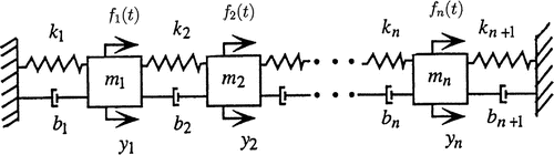
The associated initial-value problem is given by$$M\ddot{y}+B\dot{y}+Ky=f(t),y(0)=y_0,\dot{y}(0)={\dot{y}}_0$$

where $y={[y_1,\dots ,y_n]}^T$ and $f(t)={[f_1(t),\dots ,f_n(t)]}^T$ as well as$$M=\left[\begin{array}{cccc}{m}_1& & & \\ & m_2& & \\ & & m_3& & \\ & & \ddots \\ & & & m_n\end{array}\right],$$$$B=\left[\begin{array}{cccc}{b}_1+b_2& -b_2& & \\ -b_2& b_2+b_3& -b_3& & \\ & -b_3& b_3+b_4& -b_4& \\ & \ddots & \ddots & \ddots & \\ & & -b_{n-1}& b_{n-1}+b_n& -b_n\\ & & -b_n& b_n+b_{n+1}\end{array}\right],$$$$K=\left[\begin{array}{cccc}{k}_1+k_2& -k_2& & \\ -k_2& k_2+k_3& -k_3& & \\ & -k_3& k_3+k_4& -k_4& \\ & \ddots & \ddots & \ddots & \\ & & -k_{n-1}& k_{n-1}+k_n& -k_n\\ & & -k_n& k_n+k_{n+1}\end{array}\right].$$

Here, y is the displacement vector, f(t) the applied force, and M, B, and K are the mass, damping, and stiffness matrices, as the case may be.

In the state-space description, one obtains$$\dot{x}(t)=Ax(t)+b(t),x(0)=x_0,$$

with $x={[y^T,z^T]}^T,z=\dot{y}$, and $x_0={[y_0^T,z_0^T]}^T,z_0={\dot{y}}_0$, where the initial vector $x_0={[y_0^T,z_0^T]}^T$ is characterized by the mean vector $m_0$ and the covariance matrix $P_0$.

The system matrix A and the excitation vector b(t) are given by

respectively. The vector x(t) is called state vector.

The (symmetric positive semi-definite) intensity matrix $Q=Q_b$ is obtained from the (symmetric positive semi-definite) intensity matrix $Q_f$ by

See Muller and Schiehlen (1985, (9.65)) and the derivation of this relation in Kohaupt (2015b, Appendix A.5).

10.2. The transformation matrix S and the output equation $x_S(t)=Sx(t)$

We depart from the equation of motion in vector form, namely $M\ddot{y}+B\dot{y}+Ky=f(t)$, and rewrite it as$${\ddot{y}}_a(t):=\ddot{y}-M^{-1}f(t)=-M^{-1}Ky(t)-M^{-1}B\dot{y}(t).$$

Following Müller (1985, (9.56), (9.57)), for a one-mass model with base excitation, we call ${\ddot{y}}_a$ the absolute acceleration of our vibration system; it can be written as$${\ddot{y}}_a(t)=[-M^{-1}K,-M^{-1}B]\left[\begin{array}{c}y(t)\\ \dot{y}(t)\end{array}\right]=Sx(t)=:x_S(t),t\ge 0,$$

with the transformation matrix $$S=[-M^{-1}K,-M^{-1}B].$$

Our output equation therefore is$$x_S(t)=Sx(t),$$

where here $S\in I{R}^{n\times 2n}$ is a rectangular, but not a square regular matrix.

10.3. Data for the model

As of now, we specify the values as$$\begin{array}{cc}\hfill m_j& =1,j=1,\dots ,n\hfill \\ \hfill k_j& =1,j=1,\dots ,n+1\hfill \end{array}$$

and$$\begin{array}{c}\hfill b_j=\left\{\begin{array}{cc}1/2,\hfill & j\text{even}\hfill \\ 1/4,\hfill & j\text{odd}.\hfill \end{array}\right.\end{array}$$

Then,$$\begin{array}{cc}& M=E\hfill \\ \hfill & B=\left[\begin{array}{cccc}\frac{3}{4}\hfill & -\frac{1}{2}\hfill & \hfill & \\ -\frac{1}{2}\hfill & \frac{3}{4}\hfill & -\frac{1}{4}\hfill & \hfill & \\ \hfill & -\frac{1}{4}\hfill & \frac{3}{4}\hfill & -\frac{1}{2}\hfill & \\ \hfill & \hfill & \ddots \hfill & \ddots \hfill & \ddots \hfill \\ \hfill & \hfill & -\frac{1}{4}\hfill & \frac{3}{4}\hfill & -\frac{1}{2}\hfill \\ \hfill & \hfill & -\frac{1}{2}\hfill & \frac{3}{4}\hfill \end{array}\right]\hfill \end{array}$$(if n is even), and$$K=\left[\begin{array}{cccc}2\hfill & -1\hfill & \hfill & \\ -1\hfill & 2\hfill & -1\hfill & \hfill & \\ \hfill & -1\hfill & 2\hfill & -1\hfill & \\ \hfill & \hfill & \ddots \hfill & \ddots \hfill & \ddots \hfill \\ \hfill & \hfill & -1\hfill & 2\hfill & -1\hfill \\ \hfill & \hfill & -1\hfill & 2\hfill \end{array}\right].$$

We choose n = 5 in this paper so that the state-space vector x(t) has the dimension $m=2n=10$.

For $m_0$, we take$$m_0={[m_{y_0}^T,m_{z_0}^T]}^T$$

with$$m_{y_0}={[-1,1,-1,1,-1]}^T$$

and$$m_{z_0}=\left\{\begin{array}{cc}{\left[0,0,0,0,0,0\right]}^T\hfill & (\mathrm{Case}\mathrm{I})\hfill \\ {\left[-1,-1,-1,-1,-1\right]}^T\hfill & (\mathrm{Case}\mathrm{II})\hfill \end{array}\right.$$

similarly as in Kohaupt (2002) for $y_0$ and ${\dot{y}}_0$. For the $10\times 10$ matrix $P_0$, we choose$$P_0=0.01E.$$

The white-noise force vector f(t) is specified as$$f(t)={\left[0,\dots ,0;f_n(t)\right]}^T$$

so that its intensity matrix $Q_f\in I{R}^{n\times n}$ with $q_{f,nn}=:q$ has the form

We choose$$q=0.01.$$

With $M=E$, this leads to (see Kohaupt, 2015b, Appendix A.5)

10.4. Positiveness of the constants $X_{S,0}$ and ${\mathit{\phi }}_{S,0}$ (resp. $p_{S,0}$)

The eigenvalues of matrix A are given by

and$${\mathit{\lambda }}_{5+i}={\overline{\mathit{\lambda }}}_i,i=1,\dots ,5$$

where the numbering is chosen such that $Im{\mathit{\lambda }}_i>0,i=1,\dots ,5$. So,$${\mathit{\lambda }}_i\ne {\mathit{\lambda }}_j,i\ne j,i,j=1,\dots ,10.$$

Thus, matrix A is diagonalizable. Further, conditions (H1)-(H4), and (HS) are fulfilled. Moreover, we have $J_{{\mathit{\nu }}_0}=\{5\}$ and

Therefore, $q_5,{\overline{q}}_5$ are linearly independent. Thus, by Lemma A.1 and Theorem 2 resp. Theorem 6, the constants $X_{S,0}$ and ${\mathit{\phi }}_{S,0}$ are positive. Therefore, also the constant $p_{S,0}$ is positive.

10.5. Computations with the specified data

(i)	Bounds on $y={\mathrm{\Phi }}_S(t)m_0$in the vector norm ${\Vert ·\Vert }_2$Upper bounds on $y=\mathrm{\Phi }(t)m_0$ in the vector norm ${\Vert ·\Vert }_2$ for the two cases (I) and (II) of $m_0$ are given in Kohaupt (2002, Figures 2 and 3). There, we had a deterministic problem with $f(t)=0$ and the solution vector $x(t)=\mathrm{\Phi }(t)x_0$, where $x_0$ there had the same data as $m_0$ here. We mention that for the specified data, ${\mathit{\nu }}_{m_0}[A]=\mathit{\nu }[A]=\mathit{\alpha }$ in both cases (Kohaupt, 2006, p. 154) for a method to prove this. For the sake of brevity, we do not compute or plot the lower or upper bounds and thus the two-sided bounds on $y={\mathrm{\Phi }}_S(t)m_0$ but leave this to the reader.
(ii)	Computation of P and $P_0-P$ The computation of these matrices was already done in Kohaupt (2015b, Subsection 3). There, we saw that P is symmetric and $P_0-P$ symmetric and regular (but not positive definite). Matrix $P_0-P$ is needed to compute the curve $y=\Vert P_{x_S}(t)-P_S{\Vert }_2={\Vert {\mathrm{\Phi }}_S(t)(P_0-P){\mathrm{\Phi }}_S^T(t)\Vert }_2$.
(iii)	Computation of the curves $y=D_{+}^k\Vert P_{x_S}(t)-P_S{\Vert }_2=D_{+}^k{\Vert {\mathrm{\Phi }}_S(t)(P_0-P){\mathrm{\Phi }}_S^T(t)\Vert }_2$, $k=0,1,2$ The computation of $y=D_{+}^k{\Vert P_{x_S}(t)-P_S\Vert }_2$, $k=0,1,2$ for the given data is done according to Section 9 with $C=P_0-P$. The pertinent curves are illustrated in Figures 2–4. We have checked the results numerically by difference quotients. More precisely, setting $$\mathrm{\Delta }{P}_{x_S}(t):=P_{x_S}(t)-P_S,t>0,$$ and $$g(t):=\Vert \mathrm{\Delta }{P}_{x_S}{(t)\Vert }_2={\Vert P_{x_S}(t)-P_S\Vert }_2,t>0,$$ we have investigated the approximations $${\mathit{\delta }}_{h}g(t):=\frac{g(t+h)-g(t-h)}{2h}\approx D_{+}g(t),t-h\ge 0,$$ and $${\mathit{\delta }}_{\frac{h}{2}}^{2}g(t):={\mathit{\delta }}_{\frac{h}{2}}({\mathit{\delta }}_{\frac{h}{2}}g(t))=\frac{g(t+h)-2g(t)+g(t-h)}{h^2}\approx D_{+}^{2}g(t),t-h\ge 0,$$ as well as $${\mathit{\delta }}_{h}Dg(t):=\frac{Dg(t+h)-Dg(t-h)}{2h}\approx D_{+}^{2}g(t),t-h\ge 0.$$ For, e.g. $$\begin{array}{cc}\hfill t& =2.5,\hfill \\ \hfill h& ={10}^{-5},\hfill \end{array}$$ we obtain $$\begin{array}{cc}\hfill D_{+}g(t)& =D_{+}{\Vert P_{x_S}(t)-P_S\Vert }_2=-0.00789413206599,\hfill \\ \hfill {\mathit{\delta }}_{h}g(t)& ={\mathit{\delta }}_h{\Vert P_{x_S}(t)-P_S\Vert }_2=-0.00789413206470,\hfill \end{array}$$ as well as $$\begin{array}{cc}\hfill D_{+}^{2}g(t)& =D^2{\Vert P_{x_S}(t)-P_S\Vert }_2=0.00180394234645,\hfill \\ \hfill {\mathit{\delta }}_{\frac{h}{2}}^{2}g(t)& ={\mathit{\delta }}_{\frac{h}{2}}^2{\Vert P_x(t)-P\Vert }_2=0.00180268994177,\hfill \end{array}$$ and $$\begin{array}{cc}\hfill D_{+}^{2}g(t)& =D^2{\Vert P_{x_S}(t)-P_S\Vert }_2=0.00180394234645,\hfill \\ \hfill {\mathit{\delta }}_{h}Dg(t)& ={\mathit{\delta }}_{h}D{\Vert P_{x_S}(t)-P_S\Vert }_2=0.00180394235409,\hfill \end{array}$$ so that the computational results for $y=D_{+}^k{\Vert P_{x_S}(t)-P_S\Vert }_2$, $k=0,1,2$ with $t=2.5$ are well underpinned by the difference quotients. As we see, the approximation of $D_{+}^{2}g(t)=D_{+}^2{\Vert P_{x_S}(t)-P_S\Vert }_2$ by ${\mathit{\delta }}_{h}Dg(t)$ is much better than by ${\mathit{\delta }}_{\frac{h}{2}}^{2}g(t)$, which was to be expected, of course.
(iv)	Bounds on $y=P_{x_S}(t)-P_S={\mathrm{\Phi }}_S(t)(P_0-P){\mathrm{\Phi }}_S^T(t)$in the spectral norm ${\Vert ·\Vert }_2$ Let $\mathit{\alpha }:=\mathit{\nu }[A]$ be the spectral abscissa of the system matrix A. With the given data, we obtain $$\mathit{\alpha }:=\mathit{\nu }[A]=-0.05023936121946<0$$ so that the system matrix A is asymptotically stable. The upper bound on $y=\Vert P_{x_S}(t)-P_S{\Vert }_2={\Vert {\mathrm{\Phi }}_S(t)(P_0-P){\mathrm{\Phi }}_S^T(t)\Vert }_2$ is given by $y=p_{S,1}(\mathit{\epsilon })e^{2(\mathit{\alpha }+\mathit{\epsilon })t}$, $t\ge 0$. Here, $\mathit{\epsilon }=0$ can be chosen since matrix A is diagonalizable. But, in the programs, we have chosen the machine precision $\mathit{\epsilon }=eps=2^{-52}\doteq 2.2204\times {10}^{-16}$ of MATLAB in order not to be bothered by this question. With ${\mathit{\phi }}_{1,\mathit{\epsilon }}(t):=p_{S,1}(\mathit{\epsilon })e^{2(\mathit{\alpha }+\mathit{\epsilon })t},t\ge 0$, the optimal constant $p_{S,1}(\mathit{\epsilon })$ in the upper bound is obtained by the two conditions $$\begin{array}{cc}\hfill \Vert P_{x_S}(t_c)-P_S{\Vert }_2& ={\mathit{\phi }}_{1,\mathit{\epsilon }}(t_c)=p_{S,1}(\mathit{\epsilon })e^{2(\mathit{\alpha }+\mathit{\epsilon })t_c},\\ \hfill D_{+}{\Vert P_{x_S}(t_c)-P_S\Vert }_2& ={\mathit{\phi }}_{1,\mathit{\epsilon }}^{\prime }(t_c)=2(\mathit{\alpha }+\mathit{\epsilon }){\mathit{\phi }}_{1,\mathit{\epsilon }}(t_c),\end{array}$$ where $t_c$ is the place of contact between the curves. This is a system of two nonlinear equations in the two unknowns $t_c$ and $p_{S,1}(\mathit{\epsilon })$. By eliminating ${\mathit{\phi }}_{1,\mathit{\epsilon }}(t_c)$, this system is reduced to the determination of the zero of $$D_{+}\Vert P_{x_S}(t_c)-P_S{\Vert }_2-2(\mathit{\alpha }+\mathit{\epsilon }){\Vert P_{x_S}(t_c)-P_S\Vert }_2=0,$$ which is a single nonlinear equation in the single unknown $t_c$. For this, MATLAB routine fsolve was used. After $t_c$ has been computed from the above equation, the best constant $p_{S,1}(\mathit{\epsilon })$ is obtained from $$p_{S,1}(\mathit{\epsilon })={\Vert P_{x_S}(t_c)-P_S\Vert }_2{e}^{-2(\mathit{\alpha }+\mathit{\epsilon })t_c}.$$

Figure 2. Curve $y=\Vert P_{x_S}(t)-P_S{\Vert }_2,0\le t\le 5,\mathrm{\Delta }t=0.01$.

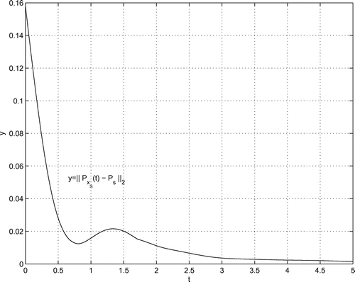
Figure 3. Right norm derivative $y=D_{+}{\Vert P_{x_S}(t)-P_S\Vert }_2,0\le t\le 5,\mathrm{\Delta }t=0.01$.

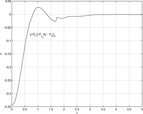
Figure 4. Second right norm derivative $y=D_{+}^2{\Vert P_{x_S}(t)-P_S\Vert }_2,0\le t\le 5,\mathrm{\Delta }t=0.01$.

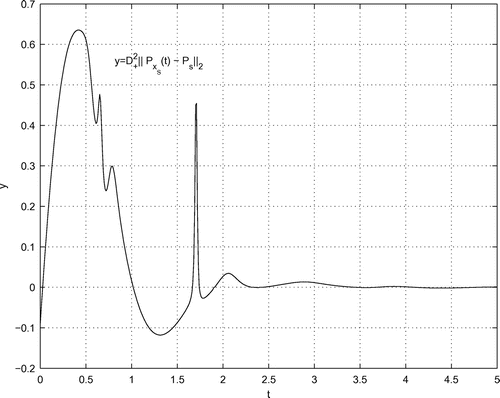
Numerical values for range [0;5] First, we consider the range [0;5]. From the initial guess $t_{c,0}=1.4$, the computations deliver the values$$\begin{array}{cc}& t_c=1.355984,\hfill \\ \hfill & p_{S,1}(\mathit{\epsilon })=0.024642.\hfill \end{array}$$

To compute the lower bound, we have to notice that the curve $y=\Vert P_{x_S}(t_c)-P_S{\Vert }_2$ has kinks like ${|t|}^{\frac{1}{2}}$ at $t=0$. This is not seen in Figures 2–5 in the range [0;5], but in Figure 6 in the range [5;25]. Therefore, the point of contact $t_s$ between the lower bound $y=M_{S,0}{e}^{2\mathit{\alpha }t}$ and the curve $y=\Vert P_{x_S}(t)-P_S{\Vert }_2$ cannot be determined by the calculus of norms, but must be computed from$${\displaystyle t_s=\underset{j=1,2,\dots }{min}{\Vert P_{x_S}(t_j)-P_S\Vert }_2,}$$

where $t_j,j=1,2,\dots$ are the local minima of $y=\Vert P_{x_S}(t_c)-P_S{\Vert }_2$. In this way, with the initial guess $t_{s,0}=3.0$, the results are$$\begin{array}{cc}& t_s=17.152006,\hfill \\ \hfill & p_{S,0}=9.403735\times {10}^{-5}.\hfill \end{array}$$

In Figure 5, the curve $y=\Vert P_{x_S}(t_c)-P_S{\Vert }_2$ along with the best upper and lower bounds are illustrated with stepsize $\mathrm{\Delta }t=0.01$. The upper bound is valid for $t\ge t_1\doteq 1.172$.

Numerical values for range [5;25] On the rage [5;25], the two-sided bounds can be better adapted to the curve $y=\Vert P_{x_S}(t)-P_S{\Vert }_2$. From the initial guess $t_{c,0}=14$, the computations deliver$$\begin{array}{cc}& t_c=14.876956,\hfill \\ \hfill & p_{S,1}(\mathit{\epsilon })=0.00164024.\hfill \end{array}$$

Further, with the initial guess $t_{s,0}=25$, we obtain$$\begin{array}{cc}& t_s=24.860534,\hfill \\ \hfill & p_{S,0}=3.548384.\hfill \end{array}$$

Figure 5. $y=\Vert P_{x_S}(t)-P_S{\Vert }_2$ along with the best upper and lower bounds on range [0;5].

In Figure 6, the curve $y=\Vert P_{x_S}(t)-P_S{\Vert }_2$ along with the best upper and lower bounds are illustrated with stepsize $\mathrm{\Delta }t=0.01$. The upper bound is valid for $t\ge t_1\doteq 6.031$.

Figure 6. $y=\Vert P_{x_S}(t)-P_S{\Vert }_2$ along with the best upper and lower bounds on range [5;25].

10.6. Computational aspects

In this subsection, we say something about the computer equipment and the computation time for some operations.

(i)

As to the computer equipment, the following hardware was available: an Intel Pentium D(3.20 GHz, 800 MHz Front-Side-Bus, 2x2MB DDR2-SDRAM with 533 MHz high-speed memories). As software package, we used MATLAB, Version 6.5.

(ii)

The computation time t of an operation was determined by the command sequence $t_i=clock;operation;t=etime(clock,t_i)$; it is put out in seconds rounded to two decimal places by Matlab. For the computation of the eigenvalues of matrix A, we used the command $[XA,DA]=eig(A)$; the pertinent computation time is less than 0.01 s. To determine $\mathrm{\Phi }(t)=e^{At}$, we employed Matlab routine expm. For the computation of the 501 values t, y, yu, yl in Figure 5, it took $t(TableforFigure5)=1.17s$. Here, t stands for the time value running from $t_0=0$ to $t_e=25$ with stepsize $\mathrm{\Delta }t=0.1$; y stands for the value of $\Vert P_{x_S}(t)-P_S{\Vert }_2$, yu for the value of the best upper bound $p_{S,1}(\mathit{\epsilon })e^{2(\mathit{\alpha }+\mathit{\epsilon })t}$ and yl for the value of the lower bound $p_{S,0}{e}^{2\mathit{\alpha }t}$. For the computation of the 2501 values t, y, yu, yl in Figure 6, it took $t(TableforFigure6)=6.35s$.

11. Conclusion

In the present paper, a linear stochastic vibration system of the form $\dot{x}(t)=Ax(t)+b(t),x(0)=x_0,$ with output equation $x_S(t)=Sx(t)$ was investigated, where A is the system matrix and b(t) white noise excitation. The output equation $x_S(t)=Sx(t)$ is viewed as a transformation of the state vector x(t) mapped by the rectangular matrix S into the output vector $x_S(t)$. If the system matrix A is asymptotically stable, then the mean vector $m_{x_S}(t)$ and the covariance matrix $P_{x_S}(t)$ both converge with $m_{x_S}(t)\to 0(t\to \infty )$ and $P_{x_S}(t)\to P_S(t\to \infty )$ for some symmetric positive (semi-)definite matrix $P_S$. This raises the question of the asymptotic behavior of both quantities. The pertinent investigations are made in the Euclidean norm ${\Vert ·\Vert }_2$ for $m_{x_S}(t)$ and in the spectral norm, also denoted by ${\Vert ·\Vert }_2$, for $P_{x_S}(t)-P_S$. The main new points are the derivation of two-sided bounds on both quantities, the determination of the right norm derivatives $D_{+}^k{\Vert P_{x_S}(t)-P_S\Vert }_2,k=0,1,2$ and, as application, the computation of the best constants in the bounds. In the presentation, the author exhibits the relations between the quantities $m_x(t)$, $P_x(t)-P$, and the formulas for $D_{+}^k{\Vert P_x(t)-P\Vert }_2$, on the one hand, and the corresponding output-related quantities $m_{x_S}(t)$, $P_{x_S}(t)-P_S$, and $D_{+}^k{\Vert P_{x_S}(t)-P_S\Vert }_2$, on the other hand. As a result, we obtain that there is a close relationship between these quantities. Special attention is paid to the positiveness of the constants in the lower bounds if the transformation matrix is only rectangular and not necessarily square and regular. In the Appendix, a sufficient algebraic condition for the positiveness of the constants in the lower bounds is derived that is independent of the initial vector and the time variable. To make sure that the (new) formulas for $D_{+}^k{\Vert P_{x_S}(t)-P_S\Vert }_2$ are correct, we have checked them by various difference quotients. They underpin the correctness of the numerical values for the specified data.

The computation time to generate the last figure with a $10\times 10$ matrix A is about 6 seconds. Of course, in engineering practice, much larger models occur. As in earlier papers, we mention that in this case engineers usually employ a method called condensation to reduce the size of the matrices.

We have shifted the details of the positiveness of the constants in the lower bounds to the Appendix in order to make the paper easier to comprehend.

The numerical values were given in order that the reader can check the results.

Altogether, the results of the paper should be of interest to applied mathematicians and particularly to engineers.

Acknowledgements

The author would like to give thanks to the anonymous referees for evaluating the paper and for comments that led to a better presentation of the paper.

Additional information

Funding

The author received no direct funding for this research.

Notes on contributors

L. Kohaupt

Ludwig Kohaupt received the equivalent to the master’s degree (Diplom-Mathematiker) in Mathematics in 1971 and the equivalent to the PhD (Dr.phil.nat.) in 1973 from the University of Frankfurt/Main. From 1974 until 1979, Kohaupt was a teacher in Mathematics and Physics at a Secondary School. During that time (from 1977 until 1979), he was also an auditor at the Technical University of Darmstadt in Engineering Subjects, such as Mechanics, and especially Dynamics. From 1979 until 1990, he joined the Mercedes-Benz car company in Stuttgart as a Computational Engineer, where he worked in areas such as Dynamics (vibration of car models), Cam Design, Gearing, and Engine Design. Then, in 1990, Dr. Kohaupt combined his preceding experiences by taking over a professorship at the Beuth University of Technology Berlin (formerly known as TFH Berlin). He retired on April 01, 2014.

Appendix 1

Algebraic conditions ensuring the positiveness of $X_{S,0}$ resp. ${\mathit{\phi }}_{S,0}$ for $S=[-M^{-1}K,-M^{-1}B]$.

We discuss two cases, namely the case of a diagonalizable matrix A and the case of a general square matrix A.

The corresponding Lemmas A.1 and A.2 will deliver sufficient algebraic criteria for the positiveness of $X_{S,0}$ and ${\mathit{\phi }}_{S,0}$, as the case may be, that are independent of the initial condition and the time, which is the important point.

The results are of interest on their own.

Case 1: Diagonalizable matrix A

Let the hypotheses (H1), (H2), and (HS) be fulfilled. Further, according to (37), we assume(A1) $$\begin{array}{c}\hfill \sum _{k\in J_{{\mathit{\nu }}_0}}S{f}_k(t)\ne 0,t\ge t_0,\end{array}$$(A1)

with$$f_k(t)=\left[\begin{array}{c}{g}_k(t)\\ h_k(t)\end{array}\right]$$

so that$$S{f}_k(t)=-M^{-1}K{g}_k(t)-M^{-1}B{h}_k(t)=-M^{-1}[K{g}_k(t)+B{h}_k(t)],k\in J_{{\mathit{\nu }}_0}.$$

Thus, (37) resp. (72) is equivalent to(A2) $$\begin{array}{c}\hfill \sum _{k\in J_{{\mathit{\nu }}_0}}[K{g}_k(t)+B{h}_k(t)]\ne 0,t\ge t_0.\end{array}$$(A2)

We have the following

Sufficient condition for ${\sum }_{k\in J_{{\mathit{\nu }}_0}}[K{g}_k(t)+B{h}_k(t)]\ne 0,t\ge t_0$:(A3) $$\begin{array}{c}\hfill K{q}_k^{(r)}+B{r}_k^{(r)},K{q}_k^{(i)}+B{r}_k^{(i)},k\in J_{{\mathit{\nu }}_0},linearlyindependent\end{array}$$(A3) (see Kohaupt, 2011, Section 5.1 for a similar case).

Lemma 3

(Some equivalences of the sufficient algebraic condition)

Let the conditions (H1), (H2), (H3), and (HS) be fulfilled. Further, let $M,B,K\in I{R}^{n\times n}$ and M be regular.

Then, the following equivalences are valid:(A4) $$\begin{array}{c}\hfill K{q}_k^{(r)}+B{r}_k^{(r)},K{q}_k^{(i)}+B{r}_k^{(i)},k\in J_{{\mathit{\nu }}_0},linearlyindependent\end{array}$$(A4) $⟺$(A5) $$\begin{array}{c}\hfill K{q}_k+B{r}_k,K{\overline{q}}_k+B{\overline{r}}_k,k\in J_{{\mathit{\nu }}_0},linearlyindependent\end{array}$$(A5) $⟺$(A6) $$\begin{array}{c}\hfill q_k{\overline{q}}_k,k\in J_{{\mathit{\nu }}_0},linearlyindependent\end{array}$$(A6) $⟺$(A7) $$\begin{array}{c}\hfill q_k^{(r)},q_k^{(i)},k\in J_{{\mathit{\nu }}_0},linearlyindependent\end{array}$$(A7)

Proof

The equivalences (75) $⟺$ (76) and (77) $⟺$ (78) are clear. Further, since(A8) $$\begin{array}{c}\hfill r_k={\mathit{\lambda }}_k{q}_k,\end{array}$$(A8) (76) is equivalent to(A9) $$\begin{array}{c}\hfill K{q}_k+{\mathit{\lambda }}_{k}B{q}_k,K{\overline{q}}_k+{\overline{\mathit{\lambda }}}_{k}B{\overline{q}}_k,k\in J_{{\mathit{\nu }}_0},linearlyindependent.\end{array}$$(A9)

Since$${\mathit{\lambda }}_k^{2}M{q}_k+{\mathit{\lambda }}_{k}B{q}_k+K{q}_k=0,{\overline{\mathit{\lambda }}}_k^{2}M{\overline{q}}_k+{\overline{\mathit{\lambda }}}_{k}B{\overline{q}}_k+K{\overline{q}}_k=0,k\in J_{{\mathit{\nu }}_0},$$(80) is equivalent to(A10) $$\begin{array}{c}\hfill -{\mathit{\lambda }}_k^{2}M{q}_k,-{\overline{\mathit{\lambda }}}_k^{2}M{\overline{q}}_k,k\in J_{{\mathit{\nu }}_0},linearlyindependent.\end{array}$$(A10)

Since ${\mathit{\lambda }}_k\ne 0$ due to (H3) and M is regular by assumption, (81) is equivalent to (77).

$\square$

Case 2: General square matrix A Let the hypotheses $(H{1}^{\prime })$, $(H{2}^{\prime })$, $(H{3}^{\prime })$, and $(H{S}^{\prime })$ be fulfilled. Further, according to (55), we assume(A11) $$\begin{array}{c}\hfill {\displaystyle \sum _{l\in J_{{\mathit{\nu }}_0}}\sum _{k=1}^{m_l}S{f}_k^{(l)}(t)\ne 0,t\ge t_0,}\end{array}$$(A11)

with$$f_k^{(l)}(t)=\left[\begin{array}{c}{g}_k^{(l)}(t)\\ h_k^{(l)}(t)\end{array}\right]$$

so that$$S{f}_k^{(l)}(t)=-M^{-1}K{g}_k^{(l)}(t)-M^{-1}B{h}_k^{(l)}(t)=-M^{-1}[K{g}_k^{(l)}(t)+B{h}_k^{(l)}(t)],k=1,\dots ,m_l,$$$l\in J_{{\mathit{\nu }}_0}$. Thus, (55) resp. (82) is equivalent to(A12) $$\begin{array}{c}\hfill {\displaystyle \sum _{l\in J_{{\mathit{\nu }}_0}}\sum _{k=1}^{m_l}[K{g}_k^{(l)}(t)+B{h}_k^{(l)}(t)]\ne 0,t\ge t_0.}\end{array}$$(A12)

We have the following

Sufficient condition for ${\displaystyle \sum _{l\in J_{{\mathit{\nu }}_0}}\sum _{k=1}^{m_l}[K{g}_k^{(l)}(t)+B{h}_k^{(l)}(t)]\ne 0,t\ge t_0}$:(A13) $$\begin{array}{c}\hfill K{q}_k^{(l,r)}+B{r}_k^{(l,r)},K{q}_k^{(l,i)}+B{r}_k^{(l,i)},k=1,\dots ,m_l,l\in J_{{\mathit{\nu }}_0},linearlyindependent\end{array}$$(A13) (see Kohaupt, 2011, Section 5.2 for a similar case).

Lemma 4

(Some equivalences of the sufficient algebraic condition) Let the hypotheses $(H{1}^{\prime })$, $(H{2}^{\prime })$, $(H{3}^{\prime })$, and $(H{S}^{\prime })$ be fulfilled. Further, let $M,B,K\in I{R}^{n\times n}$, and M be regular.

Then, the following equivalences are valid:(A14) $$\begin{array}{c}\hfill K{q}_k^{(l,r)}+B{r}_k^{(l,r)},K{q}_k^{(l,i)}+B{r}_k^{(l,i)},k=1,\dots ,m_l,l\in J_{{\mathit{\nu }}_0},linearlyindependent\end{array}$$(A14) $⟺$(A15) $$\begin{array}{c}\hfill K{q}_k^{(l)}+B{r}_k^{(l)},K{\overline{q}}_k^{(l)}+B{\overline{r}}_k^{(l)},k=1,\dots ,m_l,l\in J_{{\mathit{\nu }}_0},linearlyindependent\end{array}$$(A15) $⟺$(A16) $$\begin{array}{c}\hfill q_k^{(l)}{\overline{q}}_k^{(l)},k=1,\dots ,m_l,l\in J_{{\mathit{\nu }}_0},linearlyindependent\end{array}$$(A16) $⟺$(A17) $$\begin{array}{c}\hfill q_k^{(l,r)},q_k^{(l,i)},k=1,\dots ,m_l,l\in J_{{\mathit{\nu }}_0},linearlyindependent\end{array}$$(A17)

Proof

The equivalences (85) $⟺$ (86) and (87) $⟺$ (88) are clear.

Now we prove the equivalence of (86) and (87). From the relations(A18) $$\begin{array}{c}\hfill (A-{\mathit{\lambda }}_{l}E)p_k^{(l)}=p_{k-1}^{(l)}\end{array}$$(A18)

with(A19) $$\begin{array}{c}\hfill p_k^{(l)}=\left[\begin{array}{c}{q}_k^{(l)}\\ r_k^{(l)}\end{array}\right],\end{array}$$(A19) $k=1,\dots ,m_l,l\in J_{{\mathit{\nu }}_0}$, in a first step, we derive associated relations for $q_k^{(l)}$ and $r_k^{(l)}$, $k=1,\dots ,m_l,l\in J_{{\mathit{\nu }}_0}$. Now, (89) means

that is,(A20) $$\begin{array}{c}\hfill r_k^{(l)}={\mathit{\lambda }}_l{q}_k^{(l)}+q_{k-1}^{(l)}\end{array}$$(A20) $$-M^{-1}K{q}_k^{(l)}-M^{-1}B{r}_k^{(l)}={\mathit{\lambda }}_l{r}_k^{(l)}+r_{k-1}^{(l)}$$

or(A21) $$\begin{array}{c}\hfill K{q}_k^{(l)}+B{r}_k^{(l)}=-M[{\mathit{\lambda }}_l{r}_k^{(l)}+r_{k-1}^{(l)}],\end{array}$$(A21) $k=1,\dots ,m_l,l\in J_{{\mathit{\nu }}_0}$. Based on (93) and the assumed regularity of M, we see that (86) is equivalent to(A22) $$\begin{array}{c}\hfill {\mathit{\lambda }}_l{r}_k^{(l)}+r_{k-1}^{(l)},{\overline{\mathit{\lambda }}}_l{\overline{r}}_k^{(l)}+{\overline{r}}_{k-1}^{(l)},k=1,\dots ,m_l,l\in J_{{\mathit{\nu }}_0},linearlyindependent.\end{array}$$(A22) In the second step, we show the equivalence of (94) with the following condition:(A23) $$\begin{array}{c}\hfill r_k^{(l)}{\overline{r}}_k^{(l)},k=1,\dots ,m_l,l\in J_{{\mathit{\nu }}_0},linearlyindependent,\end{array}$$(A23)

and then in the third step, the equivalence of (95) with (87).

Equivalence of (94) and (95):

(94) $\Rightarrow$(95): So, let (94) be fulfilled. We write $r_k^{(l)}$ in the form(A24) $$\begin{array}{c}\hfill r_k^{(l)}={\mathit{\lambda }}_l{\tilde{r}}_k^{(l)}+{\tilde{r}}_{k-1}^{(l)}\end{array}$$(A24) $k=1,\dots ,m_l,l\in J_{{\mathit{\nu }}_0}$, where the ${\tilde{r}}_k^{(l)}$ are also principal vectors of stage k corresponding to the eigenvalue ${\mathit{\lambda }}_l$. This is done as follows:$$r_1^{(l)}={\mathit{\lambda }}_l{\tilde{r}}_1^{(l)}+{\tilde{r}}_0^{(l)}$$

where ${\tilde{r}}_1^{(l)}=\frac{1}{{\mathit{\lambda }}_l}{r}_1^{(l)}$ is a principal vector of stage 1 (or eigenvector) and ${\tilde{r}}_0^{(l)}=0$. Similarly,$$r_2^{(l)}={\mathit{\lambda }}_l{\tilde{r}}_2^{(l)}+{\tilde{r}}_1^{(l)}$$

where ${\tilde{r}}_2^{(l)}=\frac{1}{{\mathit{\lambda }}_l}(r_2^{(l)}-{\tilde{r}}_1^{(l)})$ is a principal vector of stage 2 corresponding to the eigenvalue ${\mathit{\lambda }}_l$.

Proceeding in this way, using induction, (96) is proven.

Therefore, apart from (94), also the following property must hold:(A25) $$\begin{array}{c}\hfill r_k^{(l)}={\mathit{\lambda }}_l{\tilde{r}}_k^{(l)}+{\tilde{r}}_{k-1}^{(l)},{\overline{r}}_k^{(l)}={\overline{\mathit{\lambda }}}_l{\overline{\tilde{r}}}_k^{(l)}+{\overline{\tilde{r}}}_{k-1}^{(l)}k=1,\dots ,m_l,l\in J_{{\mathit{\nu }}_0},linearlyindependent,\end{array}$$(A25)

which proves (95).

(95) $\Rightarrow$(94): Let (95) be fulfilled and$${\displaystyle \sum _{l\in J_{{\mathit{\nu }}_0}}\sum _{k=1}^{m_l}\left\{{\mathit{\alpha }}_k^{(l)}({\mathit{\lambda }}_l{r}_k^{(l)}+r_{k-1}^{(l)})+{\mathit{\beta }}_k^{(l)}({\overline{\mathit{\lambda }}}_l{\overline{r}}_k^{(l)}+{\overline{r}}_{k-1}^{(l)})\right\}=0.}$$

Fully written, we obtain with $r_0^{(l)}=0$,$$\begin{array}{cc}& {\displaystyle \sum _{l\in J_{{\mathit{\nu }}_0}}\left\{{\mathit{\alpha }}_1^{(l)}({\mathit{\lambda }}_l{r}_1^{(l)}+r_0^{(l)})+{\mathit{\beta }}_1^{(l)}({\overline{\mathit{\lambda }}}_l{\overline{r}}_1^{(l)}+{\overline{r}}_0^{(l)})\right.}\hfill \\ \hfill & +{\mathit{\alpha }}_2^{(l)}({\mathit{\lambda }}_l{r}_2^{(l)}+r_1^{(l)})+{\mathit{\beta }}_2^{(l)}({\overline{\mathit{\lambda }}}_l{\overline{r}}_2^{(l)}+{\overline{r}}_1^{(l)})\hfill \\ \hfill & +{\mathit{\alpha }}_3^{(l)}({\mathit{\lambda }}_l{r}_3^{(l)}+r_2^{(l)})+{\mathit{\beta }}_3^{(l)}({\overline{\mathit{\lambda }}}_l{\overline{r}}_3^{(l)}+{\overline{r}}_2^{(l)})+\dots \hfill \\ \hfill & +\left.{\mathit{\alpha }}_{m_l}^{(l)}({\mathit{\lambda }}_l{r}_{m_l}^{(l)}+r_{m_l-1}^{(l)})+{\mathit{\beta }}_{m_l}^{(l)}({\overline{\mathit{\lambda }}}_l{\overline{r}}_{m_l}^{(l)}+{\overline{r}}_{m_l-1}^{(l)})\right\}\hfill & \hfill =0\end{array}$$

or regrouping$$\begin{array}{c}\hfill {\displaystyle \sum _{l\in J_{{\mathit{\nu }}_0}}\left\{({\mathit{\alpha }}_1^{(l)}{\mathit{\lambda }}_l+{\mathit{\alpha }}_2^{(l)})r_1^{(l)}+({\mathit{\beta }}_1^{(l)}{\overline{\mathit{\lambda }}}_l+{\mathit{\beta }}_2^{(l)}){\overline{r}}_1^{(l)}\right.}\\ \hfill & +({\mathit{\alpha }}_2^{(l)}{\mathit{\lambda }}_l+{\mathit{\alpha }}_3^{(l)})r_2^{(l)}+({\mathit{\beta }}_2^{(l)}{\overline{\mathit{\lambda }}}_l+{\mathit{\beta }}_3^{(l)}){\overline{r}}_2^{(l)}+\dots \hfill \\ \hfill & +({\mathit{\alpha }}_{m_l-1}^{(l)}{\mathit{\lambda }}_l+{\mathit{\alpha }}_{m_l}^{(l)})r_{m_l-1}^{(l)}+({\mathit{\beta }}_{m_l-1}^{(l)}{\overline{\mathit{\lambda }}}_l+{\mathit{\beta }}_{m_l}^{(l)}){\overline{r}}_{m_l}^{(l)}\hfill \\ \hfill & +\left.({\mathit{\alpha }}_{m_l}^{(l)}{\mathit{\lambda }}_l)r_{m_l}^{(l)}+({\mathit{\beta }}_{m_l}^{(l)}{\overline{\mathit{\lambda }}}_l){\overline{r}}_{m_l}^{(l)}\right\}=0\hfill \end{array}$$

By assumption, from the last line, we get$${\mathit{\alpha }}_{m_l}^{(l)}{\mathit{\lambda }}_l=0,{\mathit{\beta }}_{m_l}^{(l)}{\overline{\mathit{\lambda }}}_l=0$$

or$${\mathit{\alpha }}_{m_l}^{(l)}={\mathit{\beta }}_{m_l}^{(l)}=0;$$

further,$${\mathit{\alpha }}_{m_l-1}^{(l)}{\mathit{\lambda }}_l+{\mathit{\alpha }}_{m_l}^{(l)}=0,{\mathit{\beta }}_{m_l-1}^{(l)}{\overline{\mathit{\lambda }}}_l+{\mathit{\beta }}_{m_l}^{(l)}=0,$$

leading to$${\mathit{\alpha }}_{m_l-1}^{(l)}={\mathit{\beta }}_{m_l-1}^{(l)}=0.$$

Continuing in this way, we ultimately obtain$${\mathit{\alpha }}_k^{(l)}={\mathit{\beta }}_k^{(l)}=0,k=1,\dots ,m_l,l\in J_{{\mathit{\nu }}_0},$$

so that (94) is proven.

Further, because of the representation (92), then (95) is equivalent to(A26) $$\begin{array}{c}\hfill {\mathit{\lambda }}_l{q}_k^{(l)}+q_{k-1}^{(l)},{\overline{\mathit{\lambda }}}_l{\overline{q}}_k^{(l)}+{\overline{q}}_{k-1}^{(l)},k=1,\dots ,m_l,l\in J_{{\mathit{\nu }}_0},linearlyindependent.\end{array}$$(A26)

Similarly as above, this is equivalent to (87).

On the whole, Lemma A.2 is proven.$\square$

Alternative proof for the positiveness of $X_{S,0}$ resp. ${\mathit{\phi }}_{S,0}$ when $S=[-M^{-1}K,-M^{-1}B]$

In the special case of $S=[-M^{-1}K,-M^{-1}B]$, there is an alternative proof for the positiveness of $X_{S,0}$. This alternative proof is simpler, but the foregoing one is applicable to more general forms of S.

We employ the vector resp. matrix norm ${\Vert ·\Vert }_2$ to obtain$$\begin{array}{cc}\hfill \Vert x_S{(t)\Vert }_2^2& ={\Vert Sx(t)\Vert }_2^2=\Vert -M^{-1}{Ky(t)\Vert }_2^2+{\Vert -M^{-1}B\dot{y}(t)\Vert }_2^2\hfill \\ \hfill & \ge \Vert K^{-1}{M\Vert }_2^{-2}{\Vert y(t)\Vert }_2^2+\Vert B^{-1}{M\Vert }_2^{-2}{\Vert \dot{y}(t)\Vert }_2^2\hfill \\ \hfill & \ge X_{S,2,0}^2{\Vert x(t)\Vert }_2^2\hfill \end{array}$$

with$$X_{S,2,0}^2=min\{\Vert K^{-1}{M\Vert }_2^{-2},\Vert B^{-1}M{\Vert }_2^{-2}\}$$

so that$$\Vert x_S{(t)\Vert }_2\ge X_{S,2,0}{\Vert x(t)\Vert }_2.$$

Due to the equivalence of norms in finite-dimensional spaces, this entails that for every vector norm $\Vert ·\Vert$ one has$$\Vert x_S(t)\Vert \ge X_{S,0}\Vert x(t)\Vert$$

with a positive constant $X_{S,0}$.

A similar proof for the positiveness of ${\mathit{\phi }}_{S,0}$ is possible. This is left to the reader.

References

- Achieser, N. I., & Glasman, I. M. (1968). Theorie der linearen Operatoren im Hilbert--Raum [Theory of linear operators in Hilbert space]. Berlin: Akademie-Verlag.
- Bhatia, R., & Elsner, L. (2003). Higher order logarithmic derivatives of matrices in the spectral norm. SIAM Journal on Matrix Analysis and Applications, 25, 662–668.
- Benner, P., Deni{\ss}en, J., & Kohaupt, L. (2013). Bounds on the solution of linear time-periodic systems. Proceedings in Applied Mathematics and Mechanics, 13, 447–448.
- Benner, P., Deni{\ss}en, J., & Kohaupt, L. (2016, January 12). Trigonometric spline and spectral bounds for the solution of linear time-periodic systems ( Preprint MPIMD/16-1). Magdeburg: Max Planck Institute for Dynamics of Complex Technical Systems. Retrieved from https://protect-us.mimecast.com/s/oXA1BRUQvnpoto
- Bickley, W. G., & McNamee, J. (1960). Matrix and other direct methods for the solution of linear difference equations. Philosophical Transactions of the Royal Society of London: Series A, 252, 69–131.
- Coppel, W. A. (1965). Stability and asymptotic behavior of differential equations. Boston, MA: D.C. Heath.
- Dahlquist, G. (1959). Stability and error bounds in the numerical integration of ordinary differential equations. Transactions of the Royal Institute of Technology, Stockholm, No. 130. Uppsala; Almqvist and Wiksells Boktryckeri AB.
- Desoer, Ch. A., & Haneda, H. (1972). The measure of a matrix as a tool to analyse computer algorithms for circuit analysis. IEEE Transaction on Circuit Theory, 19, 480–486.
- Golub, G. H., & van Loan, Ch F (1989). Matrix computations. Baltimore, MD: Johns Hopkins University Press.
- Guyan, R. J. (1965). Reduction of stiffness and mass matrices. AIAA Journal, 3, 380.
- Hairer, E., N{\o}rset, S. P., & Wanner, G. (1993). Solving ordinary differential equations I. Berlin: Springer-Verlag.
- Heuser, H. (1975). Funktionalanalysis [ Functional analysis]. Stuttgart: B.G. Teubner.
- Higueras, I., & García-Celayeta, B. (1999). Logarithmic norms for matrix pencils. SIAM Journal on Matrix Analysis and Applications, 20, 646–666.
- Higueras, I., & Garc\’{\i}a-Celayeta, B. (2000). How close can the logarithmic norm of a matrix pencil come to the spectral abscissa? SIAM Journal on Matrix Analysis and Applications, 22, 472–478.
- Hu, G.-D., & Hu, G.-D. (2000). A relation between the weighted logarithmic norm of a matrix and the Lyapunov equation. BIT, 40, 606–610.
- Kantorovich, L. V., & Akilov, G. P. (1982). Funktional analysis. Oxford: Pergamon Press.
- Kato, T. (1966). Perturbation theory for linear operators. New York, NY: Springer.
- Kloeden, P., & Platen, E. (1992). Numerical solution of stochastic differential equations. Springer-Verlag.
- Kohaupt, L. (1999). Second logarithmic derivative of a complex matrix in the Chebyshev norm. SIAM Journal on Matrix Analysis and Applications, 21, 382–389.
- Kohaupt, L. (2001). Differential calculus for some p-norms of the fundamental matrix with applications. Journal of Computational and Applied Mathematics, 135, 1–21.
- Kohaupt, L. (2002). Differential calculus for p-norms of complex-valued vector functions with applications. Journal of Computational and Applied Mathematics, 145, 425–457.
- Kohaupt, L. (2003). Extension and further development of the differential calculus for matrix norms with applications. Journal of Computational and Applied Mathematics, 156, 433–456.
- Kohaupt, L. (2004a). Differential calculus for the matrix norms and with applications to asymptotic bounds for periodic linear systems. International Journal of Computer Mathematics, 81, 81–101.
- Kohaupt, L. (2004b). New upper bounds for free linear and nonlinear vibration systems with applications of the differential calculus of norms. Applied Mathematical Modelling, 28, 367–388.
- Kohaupt, L. (2005). Illustration of the logarithmic derivatives by examples suitable for classroom teaching. Rocky Mountain Journal of Mathematics, 35, 1595–1629.
- Kohaupt, L. (2006). Computation of optimal two-sided bounds for the asymptotic behavior of free linear dynamical systems with application of the differential calculus of norms. Journal of Computational Mathematics and Optimization, 2, 127–173.
- Kohaupt, L. (2007a). New upper bounds for excited vibration systems with applications of the differential calculus of norms. International Journal of Computer Mathematics, 84, 1035–1057.
- Kohaupt, L. (2007b). Short overview on the development of a differential calculus of norms with applications to vibration problems (in Russian). Information Science and Control Systems, 13, 21–32. ISSN 1814-2400.
- Kohaupt, L. (2007c). Construction of a biorthogonal system of principal vectors of the matrices A and A* with applications to the initial value problem. Journal of Computational Mathematics and Optimization, 3, 163–192.
- Kohaupt, L. (2008a). Solution of the matrix eigenvalue problem with applications to the study of free linear systems. Journal of Computational and Applied Mathematics, 213, 142–165.
- Kohaupt, L. (2008b). Biorthogonalization of the principal vectors for the matrices and with application to the computation of the explicit representation of the solution of. Applied Mathematical Sciences, 2, 961–974.
- Kohaupt, L. (2008c). Solution of the vibration problem without the hypothesis or. Applied Mathematical Sciences, 2, 1989–2024.
- Kohaupt, L. (2008d). Two-sided bounds on the difference between the continuous and discrete evolution as well as on with application of the differential calculus of norms. In M. P. {\’A}lvarez (Ed.), Leading-edge applied mathematical modeling research (pp. 319–340). Nova Science. ISBN 978-1-60021-977-1.
- Kohaupt, L. (2009a, July 10--13). A short overview on the development of a differential calculus for norms with applications to vibration problems. In The 2nd International Multi-Conference on Engineering and Technological Innovation (Vol. II). Orlando, FL. ISBN-10: 1–934272-69-8, ISBN13: 978-1-934272-69-5
- Kohaupt, L. (2009b). On an invariance property of the spectral abscissa with respect to a vector. Journal of Computational Mathematics and Optimization, 5, 175–180.
- Kohaupt, L. (2009c). Contributions to the determination of optimal bounds on the solution of ordinary differential equations with vibration behavior (Habilitation Thesis, TU Freiberg, 91 pp.). Aachen: Shaker-Verlag.
- Kohaupt, L. (2010). Two-sided bounds for the asymptotic behavior of free nonlinear vibration systems with application of the differential calculus of norms. International Journal of Computer Mathematics, 87, 653–667.
- Kohaupt, L. (2010b, January). Phase diagram for norms of the solution vector of dynamical multi-degree-of-freedom systems. Lagakos, et al. (Eds.), Recent advances in applied mathematics (pp. 69–74, 27--29). American Conference on Applied Mathematics (American Math10), WSEAS Conference in Cambridge/USA at Harvard University. WSEAS Press. ISBN 978-960-474-150-2, ISSN 1790-2769.
- Kohaupt, L. (2011). Two-sided bounds on the displacement and the velocity of the vibration problem with application of the differential calculus of norms. The Open Applied Mathematics Journal, 5, 1–18.
- Kohaupt, L. (2012). Further investigations on phase diagrams for norms of the solution vector of multi-degree-of-freedom systems. Applied Mathematical Sciences, 6, 5453–5482. ISSN: 1312–885X.
- Kohaupt, L. (2013). On the vibration-suppression property and monotonicity behavior of a special weighted norm for dynamical systems. Applied Mathematics and Computation, 222, 307–330.
- Kohaupt, L. (2015a). On norm equivalence between the displacement and velocity vectors for free linear dynamical systems. Cogent Mathematics, 2, 1095699 (33 p.).
- Kohaupt, L. (2015b). Two-sided bounds on the mean vector and covariance matrix in linear stochastically excited vibration systems with application of the differential calculus of norms. Cogent Mathematics, 2, 1021603 ( 26 p).
- Kučera, V. (1974). The matrix equation A X+X B = C. SIAM Journal on Applied Mathematics, 26, 15–25.
- Lozinski\v{i}, S. M. (1958). Error estimates for the numerical integration of ordinary differential equations I (in Russian). Izv. Vys\v{s}. U\v{c}ebn. Zaved Matematika, 5, 52–90.
- Ma, E.-Ch. (1966). A finite series solution of the matrix equation A X - X B = C. SIAM Journal of Applied Mathematics, 14, 490–495.
- Müller, P. C., & Schiehlen, W. O. (1985). Linear vibrations. Dordrecht: Martinus Nijhoff.
- Niemeyer, H., & Wermuth, E. (1987). Lineare algebra [Linear algebra]. Braunschweig: Vieweg.
- Pao, C. V. (1973a). Logarithmic derivatives of a square matrix. Linear Algebra and its Applications, 6, 159–164.
- Pao, C. V. (1973b). A further remark on the logarithmic derivatives of a square matrix. Linear Algebra and its Applications, 7, 275–278.
- S{\"o}derlind, G., & Mattheij, R. M. M. (1985). Stability and asymptotic estimates in nonautonomous linear differential systems. SIAM Journal on Mathematical Analysis, 16, 69–92.
- Str{\"o}m, T. (1972). Minimization of norms and logarithmic norms by diagonal similarities. Computing, 10, 1–7.
- Str{\"o}m, T. (1975). On logarithmic norms. SIAM Journal on Numerical Analysis, 10, 741–753.
- Stummel, F., & Hainer, K. (1980). Introduction to numerical analysis. Edinburgh: Scottish Academic Press.
- Taylor, A. E. (1958). Introduction to functional analysis. New York, NY: Wiley.
- Thomson, W. T., & Dahleh, M. D. (1998). Theory of vibration with applications. Upper Saddle River, NJ: Prentice-Hall.
- Waller, H., & Krings, W. (1975). Matrizenmethoden in der Maschinen- und Bauwerksdynamik [Matrix methods in machine and building dynamics]. Mannheim: Bibliographisches Institut.
- Whidborne, J. F., & Amer, N. (2011). Computing the maximum transient energy growth. BIT Numerical Mathematics, 51, 447–457.