Picard’s iterative method for nonlinear multicomponent transport equations

Abstract

In this paper, we present a Picard’s iterative method for the solution of nonlinear multicomponent transport equations. The multicomponent transport equations are important for mixture models of the ionized and neutral particles in plasma simulations. Such mixtures deal with the so-called Stefan–Maxwell approaches for the multicomponent diffusion. The underlying nonlinearities are delicate and it is not necessary to be an analytical function of the dependent variables. The proposed solver method is based on Banach’s contraction fix-point principle that allows to solve such nonlinearities without making any use to Lagrange multipliers and constrained variations. Such an improvement allows to solve delicate nonlinear problems and we test the application to model with multicomponent transport equations.

Keywords:

• Picard’s iterative method
• variational iterative method
• multicomponent transport
• multilevel iterative method
• plasma models
• multidiffusion model
• nonlinear solver methods

AMS Subject Classifications:

• 35K25
• 35K20
• 74S10
• 70G65

Public Interest Statement

In this paper a multi component model is presented to simulate ionized and neutral particles in plasma simulations. An improved diffusion operator is presented based on the Stefan–Maxwell approach. Such nonlinear diffusion operators are solved with novel solver methods based on the Banach’s contraction fix-point principle. For higher accuracy, multilevel iterative methods are presented to solve the nonlinearities. An extension to exponential Picard’s iterative methods is discussed, which allows to split into linear and nonlinear parts. The novel schemes are tested in blow-up, Bernoulli examples.

A real-life example based on a multicomponent diffusion model is solved with the new methods. The paper also discusses future work to the novel iterative solvers.

1. Introduction

We are motivated to apply nonlinear multicomponent transport equations, which are given by delicate plasma processes.

We deal with problems of normal pressure, room temperature plasma applications, which are used for medical and technical processes. Here, the increasing importance of plasma chemistry based on the multicomponent plasma is a key factor for such a trend, see for low pressure plasma (Senega & Brinkmann, 2006) and for atmospheric pressure regimes (Tanaka, 2004). Due to the fact of the influence of the mass transfer in the multicomponent mixture, also the standard conservation laws have to be improved, such improvements are well-known in fusion research, see the modeling of in high-ionized plasmas (Igitkhanov, 2011), but only few works are done for weak-ionized plasma for atmospheric pressure regimes.

We concentrate on a diffusion reaction model for a mixture of $\text{H},{\text{H}}_2,{\text{H}}_2^{+}$ species. The model equation results in a delicate nonlinear multidiffusion equation. Such nonlinear equations are often solved with standard fix-point iteration schemes. Here, we propose a novel higher order Picard’s iterative method, which allows to accelerate the nonlinear solver based on intermediate level. Such a treatment allows to save computational time and we obtained higher order accurate results.

The paper is outlined as follows.

In Section 2, we present our mathematical model. The Picard’s iterative methods are discussed in Section 3. The numerical experiments are presented in Section 4. In the contents, that are given in Section 5, we summarize our results.

2. Mathematical model

In the following, a model is presented due to the motivation in Senega and Brinkmann (2006), which deals with a fluid dynamical description of a plasma model based on a small Knudsen number.

The Knudsen number is the ratio of the mean free path $\mathit{\lambda }$ over the typical domain size L of the apparatus. For small Knudsen numbers $Kn\approx 0.01-1.0$, we deal with a Navier–Stokes equation, where for large Knudsen numbers $Kn\ge 1.0$, we deal with the Boltzmann equations.

We deal with the following plasma model of a mixture of $\text{H},{\text{H}}_2,{\text{H}}_2^{+}$.

We take into account the dissociation and ionization reactions, which are given as: (1) $$\begin{array}{cc}& {\text{H}}_2+\text{e}{\mathit{\lambda }}_1{\text{H}}_2^{+}+2\text{e},\hfill \\ \hfill & {\text{H}}_2+\text{e}{\mathit{\lambda }}_{2}2H+\text{e},\hfill \end{array}$$(1)

where the electron temperature is given as $T_{\text{e}}=17,400$ K and the gas temperature values remain constant $T_{\text{h}}=600$ K.

Further, we have ${\mathit{\lambda }}_1=1.58{10}^{-15}{T}_{\text{e}}^{0.5}exp\left(\frac{-15.378}{T_{\text{e}}}\right)=2.082\times {10}^{-13}$ and ${\mathit{\lambda }}_2=1.413\times {10}^{-15}{T}_{\text{e}}^{2}exp\left(\frac{-4.48}{T_{\text{e}}}\right)=4.276\times {10}^{-7}$.

The diffusion coefficients are given as in the following formula:(2) $$\begin{array}{c}\hfill D_{ij}=\frac{3}{16}\frac{f_{ij}{k}_B^2{T}_i{T}_j}{p{m}_{ij}{\mathrm{\Omega }}_{ij}^{(1,1)}(T_{ij})},\end{array}$$(2)

where the parameters are: $f_{ij}$ is a correction factor of order unity, $m_{ij}=\frac{m_i{m}_j}{m_i+m_j}$ is the reduced mass, $m_i$ mass of species i, $m_j$ mass of species j, p pressure, $t_i,T_j$ the temperature of the corresponding species, and ${\mathrm{\Omega }}_{ij}^{(1,1)}$ a collision integral (Hirschfelder, Curtiss, & Bird, 1966).

We assume the following binary diffusion parameters for our experiments:(3) $$\begin{array}{cc}& D_{{\text{H}}_2,{\text{H}}_2^{+}}=0.34[{\text{cm}}^2/\text{sec}],\hfill \\ \hfill & D_{{\text{H}}_2,\text{H}}=0.21[{\text{cm}}^2/\text{sec}],\hfill \\ \hfill & D_{{\text{H}}_2^{+},\text{H}}=0.21[{\text{cm}}^2/\text{sec}].\hfill \end{array}$$(3)

We have the following underlying model: We deal with:(4) $$\begin{array}{cc}& {\mathit{\partial }}_t{\mathit{\xi }}_i+\mathrm{\nabla }·N_i=S_i,1\le i\le 3,\hfill \\ \hfill & \sum _{j=1}^3{N}_j=0,\hfill \\ \hfill & \frac{{\mathit{\xi }}_2{N}_1-{\mathit{\xi }}_1{N}_2}{D_{12}}+\frac{{\mathit{\xi }}_3{N}_1-{\mathit{\xi }}_1{N}_3}{D_{13}}=-\mathrm{\nabla }{\mathit{\xi }}_1,\hfill \\ \hfill & \frac{{\mathit{\xi }}_1{N}_2-{\mathit{\xi }}_2{N}_1}{D_{12}}+\frac{{\mathit{\xi }}_3{N}_2-{\mathit{\xi }}_2{N}_3}{D_{23}}=-\mathrm{\nabla }{\mathit{\xi }}_2,\hfill \end{array}$$(4)

and the kinetic term $S_i$ is given as:(5) $$\begin{array}{c}\hfill S_i=\sum _{j=1}^3{\mathit{\lambda }}_{i,j}{\mathit{\xi }}_j,\end{array}$$(5)

where ${\mathit{\lambda }}_{i,j}$ are the reaction rates. Further, the domain is given as $\mathrm{\Omega }\in \mathrm{I}{\mathrm{R}}^d,d\in {IN}^{+}$ with ${\mathit{\xi }}_i\in C^2$.

We decompose the diffusion and the reaction parts and apply the following: a splitting approach to our problem; we compute $n=1,\dots ,N$, $t_0,t_1,\dots ,t_n$ time steps:

The first step is given as (Diffusion step):(6) $$\begin{array}{cc}& {\mathit{\partial }}_t{\tilde{\mathit{\xi }}}_i+\mathrm{\nabla }·N_i=0,1\le i\le 3,\hfill \\ \hfill & \sum _{j=1}^3{N}_j=0,\hfill \\ \hfill & \frac{{\tilde{\mathit{\xi }}}_2{N}_1-{\tilde{\mathit{\xi }}}_1{N}_2}{D_{12}}+\frac{{\tilde{\mathit{\xi }}}_3{N}_1-{\mathit{\xi }}_1{N}_3}{D_{13}}=-\mathrm{\nabla }{\mathit{\xi }}_1,\hfill \\ \hfill & \frac{{\tilde{\mathit{\xi }}}_1{N}_2-{\tilde{\mathit{\xi }}}_2{N}_1}{D_{12}}+\frac{{\tilde{\mathit{\xi }}}_3{N}_2-{\tilde{\mathit{\xi }}}_2{N}_3}{D_{23}}=-\mathrm{\nabla }{\tilde{\mathit{\xi }}}_2,\text{for}t\in [t^n,t^{n+1}],\hfill \\ \hfill & {\tilde{\mathit{\xi }}}_i(t^n)={\mathit{\xi }}_i(t^n),i=1,2,3,\hfill \end{array}$$(6)

and the next step (Reaction step):(7) $$\begin{array}{cc}& {\mathit{\partial }}_t{\mathit{\xi }}_i=S_i,1\le i\le 3,\text{for}t\in [t^n,t^{n+1}],\hfill \\ \hfill & {\mathit{\xi }}_i(t^n)={\tilde{\mathit{\xi }}}_i(t^{n+1}),i=1,2,3.\hfill \end{array}$$(7)

Remark 1

Based on the derived model, we discuss the application of the novel nonlinear solvers. We can also generalize the schemes for more than three species.

3. Iterative method

In the following, we discuss Picard’s iterative method with different levels. Picard’s iterative methods are known to solve delicate nonlinear problems (see Ramos, 2008,2009).

In the following, we discuss the basic ideas and we develop improved Picard’s iterative methods, e.g. exponential schemes, for our special treatments.

The basic Picard’s iterative method is given as:(8) $$\begin{array}{c}\hfill u_{k+1}(x,t)=(P{u}_k)(x,t),k=0,1,2,\dots ,\end{array}$$(8)

where the Picard’s operator is given as:(9) $$\begin{array}{c}\hfill (Pu)(x,t)=u(x,t_0)+{\int }_{t_0}^{t}F(x,s,u(x,s),\mathrm{\nabla }u(x,s),\mathrm{\Delta }u(x,s))ds.\end{array}$$(9)

Picard’s operator is applied for the two-level method as:(10) $$\begin{array}{cc}\hfill u_{k+1}(x,t)& =u(x,t_0)\hfill \\ \hfill & +{\int }_{t_0}^{t}F(x,s,u_k(x,s),\mathrm{\nabla }{u}_k(x,s),\mathrm{\Delta }{u}_k(x,s))ds,k=0,1,2,\dots .\hfill \end{array}$$(10)

Further, the operator is applied for the three-level method as:(11) $$\begin{array}{cc}\hfill u_{k+1}(x,t)& =u_k(x,t)\hfill \\ \hfill & +{\int }_{t_0}^t{F}_k(s)-F_{k-1}(s)ds,k=0,1,2,\dots ,\hfill \end{array}$$(11)

where $F_k(s)=F(x,s,u_k(x,s),\mathrm{\nabla }{u}_k(x,s),\mathrm{\Delta }{u}_k(x,s))$.

Proof

We combine two two-level methods, given as:(12) $$\begin{array}{cc}\hfill u_{k+1}(x,t)& =u(x,t_0)\hfill \\ \hfill & +{\int }_{t_0}^t{F}_k(s)ds,k=0,1,2,\dots ,\hfill \end{array}$$(12)

and(13) $$\begin{array}{cc}\hfill u_k(x,t)& =u(x,t_0)\hfill \\ \hfill & +{\int }_{t_0}^t{F}_{k-1}(s)ds,k=0,1,2,\dots ,\hfill \end{array}$$(13)

where if we subtract Equation (23) with (24), we obtain:(14) $$\begin{array}{cc}\hfill u_{k+1}(x,t)& =u_k(x,t)\hfill \\ \hfill & +{\int }_{t_0}^t{F}_k(s)-F_{k-1}(s)ds,k=0,1,2,\dots ,\hfill \end{array}$$(14) $\square$

3.1. Multilevel iterative method based on Picard’s iterative method

The multilevel iterative method is given as:

Theorem 1

We have the following construction formula for the k-level iterative method based on Picard’s iterative method:

• Two-level method is given as: (15) $$\begin{array}{c}\hfill u_i(x,t)-u(x,t_0)={\int }_{t_0}^t{F}_{i-1}(s)ds.\end{array}$$(15)

• i-level method with $i\ge 3$ is given as: (16) $$\begin{array}{c}\hfill \sum _{j=0}^{\tilde{k}}{(-1)}^j\left(\begin{array}{c}\tilde{k}\\ j\end{array}\right)u_{i-j}(x,t)={\int }_{t_0}^t\sum _{j=0}^{\tilde{k}}{(-1)}^j\left(\begin{array}{c}\tilde{k}\\ j\end{array}\right)F_{i-j-1}(s)ds.\end{array}$$(16) where $\tilde{k}=i-2$.

Proof

The case $i=2$ is the standard Picard method and clear.

For the case $i\ge 3$ we have the following complete induction given as:

We start from $i=3$ (and $\tilde{k}=i-2$) and have:(17) $$\begin{array}{cc}& \sum _{j=0}^1{(-1)}^j\left(\begin{array}{c}1\\ j\end{array}\right)u_{i-j}(x,t)={\int }_{t_0}^t\sum _{j=0}^1{(-1)}^j\left(\begin{array}{c}1\\ j\end{array}\right)F_{i-j-1}(s)ds,\hfill \\ \hfill & u_i(x,t)-u_{i-1}(x,t)={\int }_{t_0}^t(F_{i-1}(s)-F_{i-2}(s))ds,\hfill \end{array}$$(17)

The induction step is given as $i\to i+1$, where we have to multiply $(u_1-u_0)$ to the i-level method as:(18) $$\begin{array}{cc}& (u_1-u_0)\sum _{j=0}^{\tilde{k}}{(-1)}^j\left(\begin{array}{c}\tilde{k}\\ j\end{array}\right)u_{i-j}(x,t)\hfill \\ \hfill & =\sum _{j=0}^{\tilde{k}}{(-1)}^j\left(\begin{array}{c}\tilde{k}\\ j\end{array}\right)u_{i+1-j}(x,t)+\sum _{j=0}^{\tilde{k}}{(-1)}^j\left(\begin{array}{c}\tilde{k}\\ j\end{array}\right)u_{i-j}(x,t)\hfill \\ \hfill & =\sum _{j=0}^{\tilde{k}+1}{(-1)}^j\left(\begin{array}{c}\tilde{k}\\ j-1\end{array}\right)u_{i-j}(x,t)+\sum _{j=0}^{\tilde{k}+1}{(-1)}^j\left(\begin{array}{c}\tilde{k}\\ j\end{array}\right)u_{i-j}(x,t)\hfill \\ \hfill & =\sum _{j=0}^{\tilde{k}+1}{(-1)}^j\left(\begin{array}{c}\tilde{k}+1\\ j\end{array}\right)u_{i-j}(x,t)\hfill \end{array}$$(18)

where $\tilde{k}=i-2$.

The same is done for the right hand side and we have proven the formula. $\square$

Remark 2

The next level methods are given as:

• Four-level method: (19) $$\begin{array}{cc}\hfill u_k(x,t)& =2u_{k-1}(x,t)-u_{k-2}(x,t)\hfill \\ \hfill & +{\int }_{t_0}^t\left(F_{k-1}(s)-2F_{k-2}(s)+F_{k-3}(s)\right)ds,k=0,1,2,\dots ,\hfill \end{array}$$(19)

• Five-level method: (20) $$\begin{array}{ccc}\hfill u_k(x,t)& =3u_{k-1}(x,t)-3u_{k-2}(x,t)+u_{k-3}(x,t)\hfill & \hfill +{\int }_{t_0}^t\left(F_{k-1}(s)-3F_{k-2}(s)+3F_{k-3}(s)-3F_{k-4}(s)\right)ds,k=0,1,2,\dots ,\end{array}$$(20)

3.2. Exponential Picard’s iterative method

In the following, we discuss an extension of Picard’s iterative method with a linear operator (exponential idea).

The exponential Picard’s iterative method is given as:(21) $$\begin{array}{c}\hfill \frac{\mathit{\partial }{u}_{k+1}(x,t)}{\mathit{\partial }t}=A{u}_{k+1}+F_k(t),k=0,1,2,\dots ,\end{array}$$(21)

where the variation of constant formula is applied and we obtain:(22) $$\begin{array}{c}\hfill u_{k+1}(x,t)=exp(At)u(x,t_0)+{\int }_{t_0}^{t}exp(A(t-s))F_k(s)ds,k=0,1,2,\dots \end{array}$$(22)

So the two-level method is given as:(23) $$\begin{array}{cc}\hfill u_{k+1}(x,t)& =exp(At)u(x,t_0)\hfill \\ \hfill & +{\int }_{t_0}^{t}exp(A(t-s))F(x,s,u_k(x,s),\mathrm{\nabla }{u}_k(x,s),\mathrm{\Delta }{u}_k(x,s))ds,k=0,1,2,\dots ,\hfill \end{array}$$(23)

Further, the three-level method is given as:(24) $$\begin{array}{cc}\hfill u_{k+1}(x,t)& =u_k(x,t)\hfill \\ \hfill & +{\int }_{t_0}^{t}exp(A(t-s))\left(F_k(s)-F_{k-1}(s)\right)ds,k=0,1,2,\dots ,\hfill \end{array}$$(24)

where $F_k(s)=F(x,s,u_k(x,s),\mathrm{\nabla }{u}_k(x,s),\mathrm{\Delta }{u}_k(x,s))$.

The multilevel iterative method is given as:

Theorem 2

We have the following construction formula for the k-level iterative method based on Picard’s iterative method:

• Two-level method is given as: (25) $$\begin{array}{c}\hfill u_i(x,t)-exp(At)u(x,t_0)={\int }_{t_0}^{t}exp(A(t-s))F_{i-1}(s)ds.\end{array}$$(25)

• k-level method with $k\ge 3$ is given as: (26) $$\begin{array}{cc}& \sum _{j=0}^{\tilde{k}}{(-1)}^j\left(\begin{array}{c}\tilde{k}\\ i\end{array}\right)u_{i-j}(x,t)\hfill \\ & ={\int }_{t_0}^{t}exp(A(t-s))\left(\sum _{j=0}^{\tilde{k}}{(-1)}^j\left(\begin{array}{c}\tilde{k}\\ j\end{array}\right)F_{i-j-1}(s)\right)ds,\hfill \end{array}$$(26) where $\tilde{k}=k-2$.

Proof

The case $k=2$ is the variation of constants with the standard Picard method and is clear.

For the case $k\ge 3$, we have the following complete induction given as in the proof of Theorem 1. $\square$

Remark 3

The next level methods are given as:

• Four-level method: (27) $$\begin{array}{cc}\hfill u_k(x,t)& =2u_{k-1}(x,t)-u_{k-2}(x,t)\hfill \\ \hfill & +{\int }_{t_0}^{t}exp(A(t-s))\left(F_{k-1}(s)-2F_{k-2}(s)+F_{k-3}(s)\right)ds,k=0,1,2,\dots ,\hfill \end{array}$$(27)

• Five-level method: (28) $$\begin{array}{cc}\hfill u_k(x,t)& =3u_{k-1}(x,t)-3u_{k-2}(x,t)+u_{k-3}(x,t)\hfill \\ \hfill & +{\int }_{t_0}^{t}exp(A(t-s))\left(F_{k-1}(s)-3F_{k-2}(s)+3F_{k-3}(s)-3F_{k-4}(s)\right)dsk=0,1,2,\dots ,\hfill \end{array}$$(28)

4. Numerical experiments

In the following experiments, we discuss the improvements of our novel Picard’s iterative methods to the standard approaches. We start with test examples of blow-up and Bernoulli’s equations, where we could compare to analytical solutions. A multicomponent model is discussed in the next steps and the benefits to the higher order multilevel methods are presented.

4.1. First numerical example: blow-up equation

As a nonlinear differential example, we chose the Bernoulli’s equation:(29) $$\begin{array}{c}\hfill \frac{\mathit{\partial }u(t)}{\mathit{\partial }t}{=\mathit{\lambda }(u(t)}^p,t\in [0,T],\text{with}u(0)=1,\end{array}$$(29)

where the analytical solution can be derived as (see also Geiser, 2008):

$u(t)={(\frac{p-1}{-C-\mathit{\lambda }t})}^{\frac{1}{p-1}}$.

When we apply $p=2$, we have

$u(t)=\frac{1}{1-\mathit{\lambda }t}$

We choose $p=2$ , $\mathit{\lambda }=-0.2$, $T=0.2$ and $u(0)=1$.

For the numerical experiments, we have the following analytical solution:(30) $$\begin{array}{cc}\hfill u_1(t)& =1+\mathit{\lambda }t,\hfill \\ \hfill u_2(t)& =1+\mathit{\lambda }t+{\mathit{\lambda }}^2{t}^2+\frac{1}{3}{\mathit{\lambda }}^3{t}^3,\hfill \\ \hfill u_3(t)& =1+\mathit{\lambda }t+{\mathit{\lambda }}^2{t}^2+{\mathit{\lambda }}^3{t}^3+\frac{5}{12}{\mathit{\lambda }}^4{t}^4\hfill \\ \hfill & +\frac{1}{3}{\mathit{\lambda }}^5{t}^5+\frac{1}{9}{\mathit{\lambda }}^6{t}^6+\frac{1}{63}{\mathit{\lambda }}^7{t}^7.\hfill \end{array}$$(30)

We apply the Picard’s iterative method, which is given in the following as a two-level method. Here, we approximate in each sub-interval $[t^n,t^{n+1}],n=0,1,\dots ,N$, the integral:(31) $$\begin{array}{c}\hfill u_{k+1,2}(t^{n+1})=u_0(t^n)+{\int }_{t^n}^{t^{n+1}}\mathit{\lambda }{u}_{k,2}^2(s)ds,k=0,1,2,\dots .\end{array}$$(31)

For the numerical integration, we apply the different Simpson’s rules of higher order.

• Simpson’s Rule: We apply the Simpson’s rule for the two-level method: (32) $$\begin{array}{cc}\hfill u_{k+1,2}(t^{n+1})& =u_0(t^n)\hfill \\ \hfill & +\mathit{\lambda }\frac{\mathrm{\Delta }t}{6}\left(u_{k,2}^2(t^{n+1})+4u_{k,2}^2(t^{n+1/2})+u_{k,2}^2(t^n)\right),k=0,1,2,\dots ,\hfill \end{array}$$(32) where $u_{k,2}(t^{n+1/2})=u_{k,2}{(}^{n+1})-\frac{1}{2}\mathrm{\Delta }t\frac{d{u}_{k,2}}{dt}(t^{n+1})=u_{k,2}{(}^{n+1})-\mathit{\lambda }\frac{1}{2}\mathrm{\Delta }t{u}_{k,2}^2(t^{n+1})$.

• 3/8 Simpson’s rule: We apply the 3/8-Simpson’s rule for the two-level method: (33) $$\begin{array}{cc}\hfill u_{k+1,2}(t^{n+1})& =u_0(t^n)\hfill \\ \hfill & +\mathit{\lambda }\frac{\mathrm{\Delta }t}{8}\left(u_{k,2}^2(t^{n+1})+3u_{k,2}^2(t^{n+1/3})+3u_{k,2}^2(t^{n+2/3})+u_{k,2}^2(t^n)\right),k=0,1,2,\dots ,\hfill \end{array}$$(33) where $$\begin{array}{cc}\hfill u_{k,2}(t^{n+1/3})& =u_{k,2}{(}^{n+1})-\frac{2}{3}\mathrm{\Delta }t\frac{d{u}_{k,2}}{dt}(t^{n+1})=u_{k,2}{(}^{n+1})-\mathit{\lambda }\frac{2}{3}\mathrm{\Delta }t{u}_{k,2}^2(t^{n+1}),\hfill \\ \hfill u_{k,2}(t^{n+2/3})& =u_{k,2}{(}^{n+1})-\frac{1}{3}\mathrm{\Delta }t\frac{d{u}_{k,2}}{dt}(t^{n+1})=u_{k,2}{(}^{n+1})-\mathit{\lambda }\frac{1}{3}\mathrm{\Delta }t{u}_{k,2}^2(t^{n+1}).\hfill \end{array}$$

Further, for the next time step, we have $u(t^{n+1})=u_{K,2}(t^{n+1})$ and K is the number of iterative steps, e.g. K= 4.

Further, the three-level method is given as a combination of two two-level methods’ means, and we have:(34) $$\begin{array}{cc}\hfill \mathrm{\Delta }{u}_{k+1,k,3}(t^{n+1})& =u_{k+1,3}(t^{n+1})-u_{k,3}(t^{n+1})\hfill \\ \hfill & ={\int }_{t^n}^{t^{n+1}}\mathit{\lambda }\left(u_{k,3}^2(s)-u_{k-1,3}^2(s)\right)ds,\hfill \\ \hfill u_{k+1,3}(t^{n+1})& =u_{k,3}(t^{n+1})+\mathrm{\Delta }{u}_{k+1,k,3}(t^{n+1})\hfill \\ \hfill & k=0,1,2,\dots ,\hfill \end{array}$$(34)

where $u_0(t)=u(t^n)$ and for $u_{1,3}(t)=u_{1,2}(t)$, we have the two-level method. Further, we apply the trapezoidal or Simpson’s rule for the numerical integration of the integrals. Further, for the next time step, we have $u(t^{n+1})=u_{K,3}(t^{n+1})$ and K is the number of iterative steps, e.g. K= 4.

Remark 4

The three-level method has the benefit of applying the numerical integration for the differences between k and $k-1$ solutions of the right-hand side, such that we can accelerate the solver process, while we skip an additional numerical integration in each step.

Based on the reference solution, we deal with the following errors:(35) $$\begin{array}{cc}\hfill E_{L_1,k,\mathrm{\Delta }t,[0,T]}& =|u_{method,k,\mathrm{\Delta }t}(t)-u_{ref,\mathrm{\Delta }t}(t)|\hfill \\ \hfill & =\sum _{n=0}^N\mathrm{\Delta }t|u_{method,k,\mathrm{\Delta }t}(t^n)-u_{ref,\mathrm{\Delta }t}(t^n)|,\hfill \end{array}$$(35)

where method is the different Picard’s methods and k is the number of iterative steps.

Figure 1. The two-level Picard’s method compared with the analytical solution.

Table 1. Comparative results of the two-level method with k iterative steps and the analytical solution for $\mathrm{\Delta }t={10}^{-2}$ and $T=1.0$

Number of iterations	$\mathrm{\Delta }t$	$er{r}_{L1}$	comp. Time
K = 1	${10}^{-1}$	$3.33\times {10}^{-2}$	$2.3611\times {10}^{-4}$
K = 2	${10}^{-1}$	$9.0912\times {10}^{-4}$	$3.1310\times {10}^{-4}$
K = 3	${10}^{-1}$	$1.1806\times {10}^{-5}$	$3.7982\times {10}^{-4}$
K = 4	${10}^{-1}$	$1.5768\times {10}^{-5}$	$4.3628\times {10}^{-4}$
K = 5	${10}^{-1}$	$1.4943\times {10}^{-5}$	$4.8248\times {10}^{-4}$
K = 6	${10}^{-1}$	$1.4968\times {10}^{-5}$	$5.2867\times {10}^{-4}$
K = 1	${10}^{-2}$	$3.33\times {10}^{-2}$	$2.3\times {10}^{-3}$
K = 2	${10}^{-2}$	$8.7588\times {10}^{-5}$	$3.1\times {10}^{-3}$
K = 3	${10}^{-2}$	$1.0439\times {10}^{-7}$	$3.8\times {10}^{-3}$
K = 4	${10}^{-2}$	$1.5461\times {10}^{-7}$	$4.5\times {10}^{-3}$
K = 5	${10}^{-2}$	$1.5385\times {10}^{-7}$	$4.8\times {10}^{-3}$
K = 6	${10}^{-2}$	$1.5385\times {10}^{-7}$	$5.3\times {10}^{-3}$
K = 1	${10}^{-3}$	$3.33\times {10}^{-2}$	$2.3611\times {10}^{-4}$
K = 2	${10}^{-3}$	$8.7256\times {10}^{-6}$	$3.1310\times {10}^{-4}$
K = 3	${10}^{-3}$	$1.0303\times {10}^{-9}$	$3.7982\times {10}^{-4}$
K = 4	${10}^{-3}$	$1.5435\times {10}^{-9}$	$4.3628\times {10}^{-4}$
K = 5	${10}^{-3}$	$1.5427\times {10}^{-9}$	$4.8248\times {10}^{-4}$
K = 6	${10}^{-3}$	$1.5427\times {10}^{-9}$	$5.2867\times {10}^{-4}$

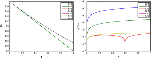
We apply the Picard’s iteration with the two-level method (see Figure 1 and Table 1).

Remark 5

Here, we see the improvement till $K=5$, while here the accuracy is reached. The reduction of the errors is done with each iterative step.

 

Figure 2. The three-level Picard’s method compared with the analytical solution.

Table 2. Comparative results of the three-level method with k iterative steps and the analytical solution for $\mathrm{\Delta }t={10}^{-2}$ and $T=1.0$

Three-Level method	Accuracy $er{r}_{L_1}$	CPU-time (sec)
$k=1$	${10}^{-4}$	$8\times {10}^{-2}$
$k=2$	${10}^{-1}$	$3\times {10}^{-2}$
$k=3$	${10}^{-1}$	$3\times {10}^{-2}$
$k=4$	${10}^{-1}$	$3\times {10}^{-2}$
$k=5$	${10}^{-1}$	$3\times {10}^{-2}$

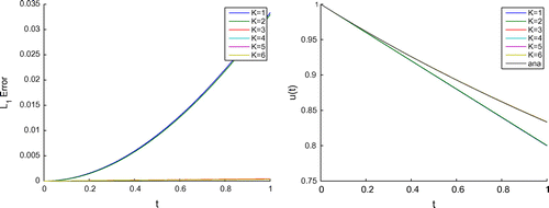
We apply the Picard’s iteration with the three-level method (see Figure 2 and Table 2).

Remark 6

Here, we see the improvement till $K=4$, while here the accuracy is reached. The reduction of the errors is done with each iterative step.

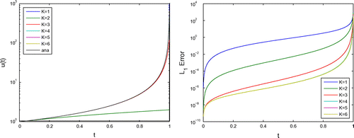
We apply the blow-up experiment with $\mathit{\lambda }=0.999$ and obtain the following solutions. The Picard’s iteration with the two-Level method is given in Figure 3 for $\mathit{\lambda }=0.999$.

Figure 3. The two-level Picard’s method compared with the analytical solution.

Figure 4. The three-level Picard’s method compared with the analytical solution.

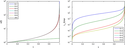
The Picard’s iteration with the three-level method is given in Figure 4 for $\mathit{\lambda }=0.999$.

Remark 7

We discussed the multilevel Picard’s method with different iterative steps to a blow-up problem. We saw that we obtain high accurate solutions with $k\approx 3-5$ iterative steps and that a three-level method can obtain faster numerical results.

4.2. Second numerical example: Bernoulli’s equation

As a nonlinear differential example, we chose the Bernoulli’s equation:(36) $$\begin{array}{c}\hfill \frac{\mathit{\partial }u(t)}{\mathit{\partial }t}=({\mathit{\lambda }}_1+{\mathit{\lambda }}_3)u(t)+({\mathit{\lambda }}_2+{\mathit{\lambda }}_4){(u(t))}^p,t\in [0,T],\text{with}u(0)=1,\end{array}$$(36)

where the analytical solution can be derived as (see also Geiser, 2008):$$u(t)=exp(({\mathit{\lambda }}_1+{\mathit{\lambda }}_3)t){\left[-\frac{{\mathit{\lambda }}_2+{\mathit{\lambda }}_4}{{\mathit{\lambda }}_1+{\mathit{\lambda }}_3}exp(({\mathit{\lambda }}_1+{\mathit{\lambda }}_3)(p-1)t)+c\right]}^{1/(1-p)}.$$

Using $u(0)=1$, we find that $c=1+\frac{{\mathit{\lambda }}_2+{\mathit{\lambda }}_4}{{\mathit{\lambda }}_1+{\mathit{\lambda }}_3}$, so$$u(t)=exp(({\mathit{\lambda }}_1+{\mathit{\lambda }}_3)t){\left\{1+\frac{{\mathit{\lambda }}_2+{\mathit{\lambda }}_4}{{\mathit{\lambda }}_1+{\mathit{\lambda }}_3}\left[1-exp(({\mathit{\lambda }}_1+{\mathit{\lambda }}_3)(p-1)t)\right]\right\}}^{1/(1-p)}.$$

We choose $p=2$ , ${\mathit{\lambda }}_1=-1$, ${\mathit{\lambda }}_2=-0.5$, ${\mathit{\lambda }}_3=-1$, ${\mathit{\lambda }}_4=-1$ , $T=0.2$, and $u(0)=1$.

We apply the Picard’s iterative method based on approximating in each sub-interval $[t^n,t^{n+1}],n=0,1,\dots ,N$, which is given as:

• Two-level method is given as: (37) $$\begin{array}{cc}\hfill u_{k+1}(t^{n+1})& =exp(({\mathit{\lambda }}_1+{\mathit{\lambda }}_3)\mathrm{\Delta }t)u(t^n)\hfill \\ \hfill & +{\int }_{t^n}^{t^{n+1}}exp(({\mathit{\lambda }}_1+{\mathit{\lambda }}_3)(t^{n+1}-s))\left(({\mathit{\lambda }}_2+{\mathit{\lambda }}_4)u_k^p(s)\right)ds,k=1,2,\dots ,\hfill \end{array}$$(37) where for $k=0$; we have: (38) $$\begin{array}{cc}\hfill u_1(t^{n+1})& =exp(({\mathit{\lambda }}_1+{\mathit{\lambda }}_3)\mathrm{\Delta }t)u(t^n)\hfill \\ \hfill & +{\int }_{t^n}^{t^{n+1}}exp(({\mathit{\lambda }}_1+{\mathit{\lambda }}_3)(t^{n+1}-s))({\mathit{\lambda }}_2+{\mathit{\lambda }}_4)u_0^p(s)ds,\hfill \end{array}$$(38) with the time step $\mathrm{\Delta }t=t^{n+1}-t^n$. We apply the following numerical integration rules:

• Simpson’s rule: We apply the Simpson’s rule for the two-level method: (39) $$\begin{array}{cc}\hfill u_{k+1,2}(t^{n+1})& =exp(({\mathit{\lambda }}_1+{\mathit{\lambda }}_3)\mathrm{\Delta }t)u_0(t^n)\hfill \\ \hfill & +({\mathit{\lambda }}_2+{\mathit{\lambda }}_4)\frac{\mathrm{\Delta }t}{6}\left(u_{k,2}^p(t^{n+1})+4exp(({\mathit{\lambda }}_1+{\mathit{\lambda }}_3)\mathrm{\Delta }t/2)u_{k,2}^p(t^{n+1/2})\right.\hfill \\ \hfill & \left.+exp(({\mathit{\lambda }}_1+{\mathit{\lambda }}_3)\mathrm{\Delta }t)u_{k,2}^p(t^n)\right),k=0,1,2,\dots ,\hfill \end{array}$$(39) where we have the intermediate solution as: (40) $$\begin{array}{cc}\hfill u_{k,2}(t^{n+1/2})& =u_{k,2}(t^{n+1})-\frac{1}{2}\mathrm{\Delta }t\frac{d{u}_{k,2}}{dt}(t^{n+1})\hfill \\ \hfill & =u_{k,2}(t^{n+1})-\frac{1}{2}\mathrm{\Delta }t\left(({\mathit{\lambda }}_1+{\mathit{\lambda }}_3)u_{k,2}(t^{n+1})+({\mathit{\lambda }}_2+{\mathit{\lambda }}_4){(u_{k,2}{(}^{n+1}))}^p\right).\hfill \end{array}$$(40)

• 3/8 Simpson’s rule: We apply the 3/8-Simpson’s rule for the two-level method: (41) $$\begin{array}{cc}\hfill u_{k+1,2}(t^{n+1})& =exp(({\mathit{\lambda }}_1+{\mathit{\lambda }}_3)\mathrm{\Delta }t)u_0(t^n)\hfill \\ \hfill & +({\mathit{\lambda }}_2+{\mathit{\lambda }}_4)\frac{\mathrm{\Delta }t}{8}\left(u_{k,2}^p(t^{n+1})+3exp(({\mathit{\lambda }}_1+{\mathit{\lambda }}_3)\mathrm{\Delta }t/3)u_{k,2}^p(t^{n+2/3})\right.\hfill \\ \hfill & \left.+3exp(({\mathit{\lambda }}_1+{\mathit{\lambda }}_3)2\mathrm{\Delta }t/3)u_{k,2}^p(t^{n+1/3})+exp(({\mathit{\lambda }}_1+{\mathit{\lambda }}_3)\mathrm{\Delta }t)u_{k,2}^p(t^n)\right),k=0,1,2,\dots ,\hfill \end{array}$$(41) where $$\begin{array}{cc}\hfill u_{k,2}(t^{n+1/3})& =u_{k,2}{(}^{n+1})-\frac{2}{3}\mathrm{\Delta }t\frac{d{u}_{k,2}}{dt}(t^{n+1})=u_{k,2}{(}^{n+1})-\mathit{\lambda }\frac{2}{3}\mathrm{\Delta }t{u}_{k,2}^2(t^{n+1}),\hfill \\ \hfill u_{k,2}(t^{n+2/3})& =u_{k,2}{(}^{n+1})-\frac{1}{3}\mathrm{\Delta }t\frac{d{u}_{k,2}}{dt}(t^{n+1})=u_{k,2}{(}^{n+1})-\mathit{\lambda }\frac{1}{3}\mathrm{\Delta }t{u}_{k,2}^2(t^{n+1}).\hfill \end{array}$$

• Three-level method is given as: Further, the three-level method is given as a combination of two two-level methods’ means; we have: (42) $$\begin{array}{cc}\hfill \mathrm{\Delta }{u}_{k+1,k,3}(t^{n+1})& =u_{k+1,3}(t^{n+1})-u_{k,3}(t^{n+1})\hfill \\ \hfill & =({\mathit{\lambda }}_2+{\mathit{\lambda }}_4){\int }_{t^n}^{t^{n+1}}exp(({\mathit{\lambda }}_1+{\mathit{\lambda }}_3)(t-s))\left(u_k^p(s)-u_{k-1}^p(s)\right)ds,\hfill \\ \hfill u_{k+1,3}(t^{n+1})& =u_{k,3}(t^{n+1})+\mathrm{\Delta }{u}_{k+1,k,3}(t^{n+1}),k=0,1,2,\dots ,\hfill \end{array}$$(42) where $u_0(t)=u(t^n)$ and for $u_{1,3}(t)=u_{1,2}(t)$, we have the two-level method. Further, we apply the trapezoidal or Simpson’s rule for the numerical integration of the integrals. Further, for the next time step, we have $u(t^{n+1})=u_{K,3}(t^{n+1})$ and K is the number of iterative steps, e.g. K = 4. (43) $$\begin{array}{cc}\hfill u_{k+1}(t^{n+1})& =u_k(t^{n+1})\hfill \\ \hfill & +{\int }_{t^n}^{t^{n+1}}exp(({\mathit{\lambda }}_1+{\mathit{\lambda }}_3)(t-s))\left(({\mathit{\lambda }}_2+{\mathit{\lambda }}_4)u_k^p(s)-({\mathit{\lambda }}_2+{\mathit{\lambda }}_4)u_{k-1}^p(s)\right)ds,\hfill \\ \hfill & k=0,1,2,\dots ,\hfill \end{array}$$(43) where $u_0(t)=u(t^n)$ and $$u_1(t)=exp(({\mathit{\lambda }}_1+{\mathit{\lambda }}_3)(t-t^n))u(t^n)+{\int }_{t^n}^{t}exp(({\mathit{\lambda }}_1+{\mathit{\lambda }}_3)(t-s))({\mathit{\lambda }}_2+{\mathit{\lambda }}_4)u_0^p(s)ds$$

We apply the trapezoidal or Simpson’s rule for the numerical integration of the integrals.

Remark 8

If we apply only the trapezoidal rule, we obtain less accurate results while we skip the term $exp(({\mathit{\lambda }}_1+{\mathit{\lambda }}_3)(\mathrm{\Delta }t))({\mathit{\lambda }}_2+{\mathit{\lambda }}_4)(u_k^p(t^n)-u_{k-1}^p(t^n))=0$, such that it is important to have with $k=2$ a third-order integration method, e.g. the Simpson’s rule.

Based on the reference solution, we deal with the following errors:(44) $$\begin{array}{cc}\hfill E_{L_1,k,\mathrm{\Delta }t,[0,T]}& =|u_{method,k,\mathrm{\Delta }t}(t)-u_{ref,\mathrm{\Delta }t}(t)|\hfill \\ \hfill & =\sum _{n=0}^N\mathrm{\Delta }t|u_{method,k,\mathrm{\Delta }t}(t^n)-u_{ref,\mathrm{\Delta }t}(t^n)|,\hfill \end{array}$$(44)

where method is the different Picard’s methods and k is the number of iterative steps.

Further, we deal with different time steps $\mathrm{\Delta }t=\mathrm{\Delta }{t}_{CFL},\mathrm{\Delta }{t}_{CFL}/2,\mathrm{\Delta }{t}_{CFL}/4$.

A restriction based on the CFL condition is not necessary, while we have a numerical integration, but for more accurate results, this can help. The CFL condition is given as:(45) $$\begin{array}{c}\hfill \mathrm{\Delta }t\le \frac{1}{|({\mathit{\lambda }}_1+{\mathit{\lambda }}_2)+({\mathit{\lambda }}_3+{\mathit{\lambda }}_4)u_0^{p-1}|}\end{array}$$(45)

where we assume $u^{n+1}(t)\le u^n,\forall t\in [0,T]$ and $u_0$ is the initial solution.

For another accurate solution, we can integrate:

We have given:(46) $$\begin{array}{cc}\hfill u_{k+1}(t^{n+1})& =u_k(t^{n+1})\hfill \\ \hfill & +{\int }_{t^n}^{t^{n+1}}exp(({\mathit{\lambda }}_1+{\mathit{\lambda }}_3)(t-s))\left(({\mathit{\lambda }}_2+{\mathit{\lambda }}_4)u_k^p(s)-({\mathit{\lambda }}_2+{\mathit{\lambda }}_4)u_{k-1}^p(s)\right)ds\hfill \\ \hfill & =u_k(t^{n+1})+\mathrm{\Delta }t{\mathit{\varphi }}_1(\mathrm{\Delta }t(({\mathit{\lambda }}_1+{\mathit{\lambda }}_3)))g(t^n)+\frac{\mathrm{\Delta }{t}^2}{2}{\mathit{\varphi }}_2(\mathrm{\Delta }t(({\mathit{\lambda }}_1+{\mathit{\lambda }}_3)))g^{\prime }(t^n)\hfill \\ \hfill & +O(\mathrm{\Delta }{t}^3),\hfill \end{array}$$(46)

where(47) $$\begin{array}{cc}\hfill g(t^n)& =({\mathit{\lambda }}_2+{\mathit{\lambda }}_4)\left(u_k^p(t^n)-u_{k-1}^p(t^n)\right)\hfill \\ \hfill g^{\prime }(t^n)& =({\mathit{\lambda }}_2+{\mathit{\lambda }}_4)p\left(({\mathit{\lambda }}_1+{\mathit{\lambda }}_3)(u_k^p(t^n)-u_{k-1}^p(t^n))\right.\hfill \\ \hfill & +\left.({\mathit{\lambda }}_2+{\mathit{\lambda }}_4)(u_k^{p-1}(t^n)u_{k-1}^p(t^n)-u_{k-1}^p(t^n)u_{k-2}^p(t^n))\right).\hfill \end{array}$$(47)

Further, we have:(48) $$\begin{array}{cc}\hfill {\mathit{\varphi }}_1(hA)& =\frac{1}{h}{\int }_0^{h}exp((h-\mathit{\tau })A)d\mathit{\tau },\hfill \\ \hfill {\mathit{\varphi }}_i(hA)& =\frac{1}{h^i}{\int }_0^{h}exp((h-\mathit{\tau })A)\frac{{\mathit{\tau }}^{i-1}}{(i-1)!}d\mathit{\tau },i\ge 1,\hfill \end{array}$$(48)

and we apply to our formulas:(49) $$\begin{array}{cc}\hfill {\mathit{\varphi }}_1(\mathrm{\Delta }t({\mathit{\lambda }}_1+{\mathit{\lambda }}_3))& =\frac{1}{\mathrm{\Delta }t({\mathit{\lambda }}_1+{\mathit{\lambda }}_3)}(exp(\mathrm{\Delta }t({\mathit{\lambda }}_1+{\mathit{\lambda }}_3))-1),\hfill \\ \hfill {\mathit{\varphi }}_2(\mathrm{\Delta }t({\mathit{\lambda }}_1+{\mathit{\lambda }}_3))& =\frac{1}{{(\mathrm{\Delta }t({\mathit{\lambda }}_1+{\mathit{\lambda }}_3))}^2}(exp(\mathrm{\Delta }t({\mathit{\lambda }}_1+{\mathit{\lambda }}_3))-1)\hfill \\ \hfill & -\frac{1}{\mathrm{\Delta }t({\mathit{\lambda }}_1+{\mathit{\lambda }}_3)}.\hfill \end{array}$$(49)

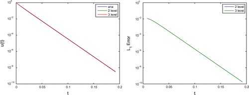
We apply the Picard’s iteration and compared to the analytical solutions, we obtain the following result in Figure 5.

Figure 5. The three-level Picard’s method compared with the analytical solution (left side: solutions, right side: errors between analytical and numerical methods).

Remark 9

We saw marginal difference between the two- and three-level Picard’s methods with different iterative steps $k=1,2,5,10$. At least, it is important to deal with more than $k\approx 3$ iterative steps. Further, it is necessary to deal with accurate numerical integration methods to save the accuracy of the multilevel nonlinear methods, meaning we applied at minimum third- or fourth-order accurate methods.

4.3. Multicomponent diffusion model

We deal with the plasma model that we presented in Section 2. The multicomponent diffusion model, which is nonlinear in the diffusion operator, solves with the multilevel Picard’s method.

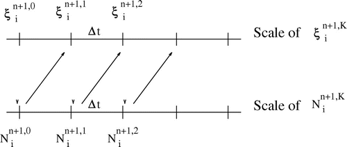
In the following, we present a three-step method, which is based on the idea of only updating the fix-point results.

To circumvent the exponential functions, we could apply for our nonlinear method a Picard’s iterative method, which is based on the following idea.

The nonlinear equation is given as:(50) $$\begin{array}{c}\hfill {\mathit{\partial }}_t{\mathit{\xi }}_i=-\mathrm{\nabla }{N}_i({\mathit{\xi }}_i),{\mathit{\xi }}_i(0)={\mathit{\xi }}_{i,0},\end{array}$$(50) ; we apply the three-step method given as:(51) $$\begin{array}{c}\hfill {\mathit{\xi }}_{i,k}(t)={\mathit{\xi }}_{i,k-1}(t)+{\int }_0^t\left(-\mathrm{\nabla }{N}_i({\mathit{\xi }}_{i,k-1}(s))+-\mathrm{\nabla }{N}_i({\mathit{\xi }}_{i,k-2}(s))\right)ds\end{array}$$(51)

where the initialization is given with the initial function ${\mathit{\xi }}_{i,0}(t)={\mathit{\xi }}_i(0)$ and the first iteration is done previously.

The explicit form of the algorithm with an explicit Euler time discretization is given as:

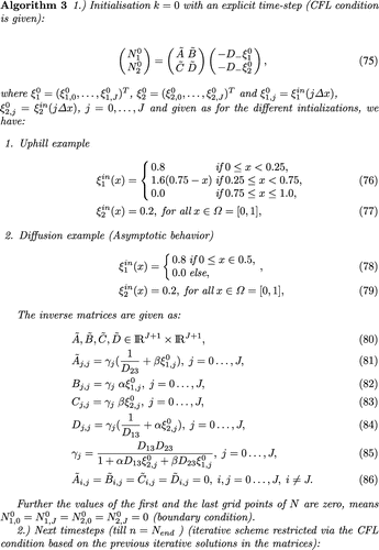
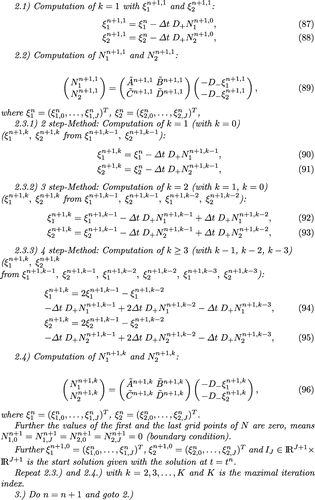
The computation of the inverse matrices is given as:(62) $$\begin{array}{cc}& {\tilde{A}}^{n+1,k-1},{\tilde{B}}^{n+1,k-1},{\tilde{C}}^{n+1,k-1},{\tilde{D}}^{n+1,k-1}\in \mathrm{I}{\mathrm{R}}^{J+1}\times \mathrm{I}{\mathrm{R}}^{J+1},\hfill \\ \hfill & {\tilde{A}}_{j,j}^{n+1,k-1}={\mathit{\gamma }}_j(\frac{1}{D_{23}}+\mathit{\beta }{\mathit{\xi }}_{1,j}^{n+1,k-1}),j=0\dots ,J,\hfill \\ \hfill & B_{j,j}^{n+1,k-1}={\mathit{\gamma }}_j\mathit{\alpha }{\mathit{\xi }}_{1,j}^{n+1,k-1},j=0\dots ,J,\hfill \\ \hfill & C_{j,j}^{n+1,k-1}={\mathit{\gamma }}_j\mathit{\beta }{\mathit{\xi }}_{2,j}^{n+1,k-1},j=0\dots ,J,\hfill \\ \hfill & D_{j,j}^{n+1,k-1}={\mathit{\gamma }}_j(\frac{1}{D_{13}}+\mathit{\alpha }{\mathit{\xi }}_{2,j}^{n+1,k-1}),j=0\dots ,J,\hfill \\ \hfill & {\mathit{\gamma }}_j=\frac{D_{13}{D}_{23}}{1+\mathit{\alpha }{D}_{13}{\mathit{\xi }}_{2,j}^{n+1,k-1}+\mathit{\beta }{D}_{23}{\mathit{\xi }}_{1,j}^{n+1,k-1}},j=0\dots ,J,\hfill \\ \hfill & {\tilde{A}}_{i,j}^{n+1,k-1}={\tilde{B}}_{i,j}^{n+1,k-1}={\tilde{C}}_{i,j}^{n+1,k-1}={\tilde{D}}_{i,j}^{n+1,k-1}=0,\hfill \\ \hfill & i,j=0\dots ,J,i\ne J.\hfill \end{array}$$(62)

The numerical errors of the different schemes are given in Figure 6.

Figure 6. The numerical error of general Picard’s fix-point method and a reference solution (fourth-order RK-method with fine time steps).

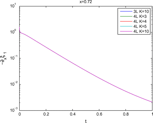
The numerical solution of the three- and four-level Picard’s fix-point schemes with different iterative steps is given in Figure 7.

Figure 7. The numerical solution of the three- and four-level Picard’s fix-point methods with different iterative steps.

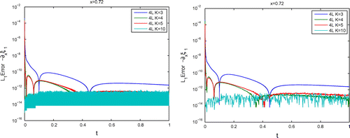
The numerical errors of the four-level Picard’s fix-point schemes compared with a reference solution of fine time steps of a three-level method (see Figure 8).

Figure 8. The figures present the numerical $L_1$-error between the four-level Picard’s fix-point scheme and the reference solution for different iterative steps (left figure: high resolution of the error, right figure: low resolution based on averaging the high oscillating errors).

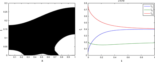
The solutions of the numerical experiments are given in Figure 9.

Figure 9. The figures present the numerical solutions of the uphill experiment (left side) and the concentrations at spatial point $x=0.72$ with a four-level Picard’s fix-point scheme computed (right side).

Remark 10

We tested all different level properties, meaning three-level and four-level Picard’s fix-point schemes, with different iterative step sizes, meaning $k=3,4,5,10$. For all applications, we saw only marginal differences, such that a three-level method is sufficient to resolve the nonlinear problem.

5. Conclusions and discussion

We present the coupled model for a multicomponent transport model, which can be applied for solving nonlinear diffusion equations, e.g. for multicomponent plasma transport models. The Picard’s methods are flexible and we could derive multilevel methods, with exponential treatments. The benefit of the methods is to resolve the nonlinearity with more accuracy based on the intermediate levels. Here, we present the improvements based on the blow-up problems and the Bernoulli’s equation. In multidiffusion applications, we saw the benefit of such methods in a fast resolution of the nonlinear diffusion and a decomposition on slow and fast time scales. Overall, the flexibility of such Picard’s methods is important to solve multicomponent problems.

Additional information

Funding

The author received no direct funding for this research.

Notes on contributors

Juergen Geiser

Juergen Geiser , researcher and lecturer at the Ruhr-University of Bochum, Germany, has been involved in teaching and research projects and has collaborated with engineering and physicist groups on numerical modeling of technical and physical models. The research activity refers to the mathematical modeling, numerics, and analysis of transport and flow problems in engineering applications, e.g. groundwater modeling and plasma modeling. He is a specialist in multiscale solvers and iterative solvers and most of the topics of the special issue. Moreover, Juergen Geiser is the author of scientific books and editor of various scientific journals and has thus able to manage the editorial activity. He is also a visiting professor at the Centrale Supelec in the laboratory: Mathematics in Interaction with Computer Sciences, Chatenay-Malabry, Cedex, France.

References

- Geiser, J. (2008). Iterative operator-splitting methods with higher order time-integration methods and applications for parabolic partial differential equations. Journal of Computational and Applied Mathematics, 217, 227–242.
- Hirschfelder, J. O., Curtiss, Ch. F., & Bird, R. B. (1966). Molecular theory of gases and liquids (Chemistry) (1st ed.).Wiley.
- Igitkhanov, Y. (2011). Modelling of multi-component plasma for TOKES (KIT Scientific Report Nr. 7564). Karlsruhe: Institut für Hochleistungsimpuls- und Mikrowellentechnik (IHM), KIT Scientific Publishing.
- Ramos, J. I. (2008). On the variational iteration method and other iterative techniques for nonlinear differential equations. Applied Mathematics and Computation, 199, 39–69.
- Ramos, J. I. (2009). Picard’s iterative method for nonlinear advection reaction-diffusion equations. Applied Mathematics and Computation, 215, 1526–1536.
- Senega, T. K., & Brinkmann, R. P. (2006). A multi-component transport model for non-equilibrium low-temperature low-pressure plasmas. Journal of Physics D: Applied Physics, 39, 1606–1618.
- Tanaka, Y. (2004). Two-temperature chemically non-equilibrium modelling of high-power Ar-N2 inductively coupled plasmas at atmospheric pressure. Journal of Physics D: Applied Physics, 37, 1190–1205.