Exact traveling wave solutions for the generalized Hirota-Satsuma couple KdV system using the exp(−φ(ξ))-expansion method

Abstract

In this research, we find the exact traveling wave solutions involving parameters of the generalized Hirota-Satsuma couple KdV system according to the exp$(-\mathit{\phi }(\mathit{\xi }))$-expansion method and when these parameters are taken to be special values we can obtain the solitary wave solutions which is derived from the exact traveling wave solutions. It is shown that the proposed method provides a more powerful mathematical tool for constructing exact traveling wave solutions for many other nonlinear evolution equations.

Keywords:

• the exp$(-\mathit{\phi }(\mathit{\xi }))$-expansion method
• the generalized Hirota-Satsuma couple KdV system
• traveling wave solutions
• solitary wave solutions

AMS Subject Classifications:

• 35A05
• 35A20
• 65K99
• 65Z05
• 76R50
• 70K70

Public Interest Statement

In this paper, we use the exp$(-\mathit{\phi }(\mathit{\xi }))$-expansion method to find the exact and solitary wave solutions of the generalized Hirota-Satsuma couple KdV system. The exact traveling wave solutions are obtained from the explicit solutions by choosing the particular value of the physical parameters. So, we can choose appropriate value of the physical parameters to obtain exact solutions we need in varied instances. There are various types of traveling wave solutions that are of particular interest in solitary wave theory.

1. Introduction

No one can deny the important role which played by the nonlinear partial differential equations in the description of many and a wide variety of phenomena not only in physical phenomena, but also in plasma, fluid mechanics, optical fibers, solid state physics, chemical kinetics, and geochemistry phenomena. So that, during the past five decades, a lot of method was discovered by a diverse group of scientists to solve the nonlinear partial differential equations. Such methods are tanh–sech method (Malfliet, 1992; Malfliet & Hereman, 1996; Wazwaz, 2004a), extended tanh method (Abdelrahman, Zahran, & Khater, 2015; El-Wakil & Abdou, 2007; Fan, 2000), sine–cosine method (Wazwaz, 2005,2004b; Yan, 1996), homogeneous balance method (Fan & Zhang, 1998; Wang, 1996), F-expansion method (Ren & Zhang, 2006; Zahran & Khater, 2014a; Zhang, Wang, Wang, & Fang, 2006), exp-function method (Aminikhad, Moosaei, & Hajipour, 2009; He & Wu, 2006), trigonometric function series method (Zhang, 2008), $(\frac{G^{{}^{\prime }}}{G})-$ expansion method (Khater, 2015; Wang, Zhang, & Li, 2008; Zahran & Khater, 2014b; Zhang, Tong, & Wang, 2008), Jacobi elliptic function method (Dai & Zhang, 2006; Fan & Zhang, 2002; Liu, Fu, Liu, & Zhao, 2001; Zahran & Khater, 2014c), The exp$(-\mathit{\phi }(\mathit{\xi }))$-expansion method (Abdelrahman, Zahran, & Khater, 2014; Islam, Nur Alam, Kazi Sazzad Hossain, Harun-Or-Roshid, & Ali Akbar, 2013; Rahman, Nur Alam, Harun-Or-Roshid, Akter, & Ali Akbar, 2014), and so on.

The objective of this article was to apply The exp$(-\mathit{\phi }(\mathit{\xi }))$-expansion method for finding the exact traveling wave solution of the generalized Hirota-Satsuma couple KdV system which play an important role in mathematical physics.

The rest of this paper is organized as follows: In Section 2, we give the description of The exp$(-\mathit{\phi }(\mathit{\xi }))$-expansion method. In Section 3, we use this method to find the exact solutions of the nonlinear evolution equations pointed out above. In Section 5, conclusions are given.

2. Description of method

Consider the following nonlinear evolution equation(2.1) $$\begin{array}{c}\hfill F(u,u_t,u_x,u_{tt},u_{xx},\dots )=0,\end{array}$$(2.1)

where F is a polynomial in u(x, t) and its partial derivatives in which the highest order derivatives and nonlinear terms are involved. In the following, we give the main steps of this method

Step 1. We use the wave transformation(2.2) $$\begin{array}{c}\hfill u(x,t)=u(\mathit{\xi }),\mathit{\xi }=x-ct,\end{array}$$(2.2)

where c is a positive constant, to reduce Equation (2.1) to the following ODE:(2.3) $$\begin{array}{c}\hfill P(u,u^{\prime },u^{″},u^{″\prime },\dots )=0,\end{array}$$(2.3)

where P is a polynomial in $u(\mathit{\xi })$ and its total derivatives, while ${}^{\prime }={\frac{d}{d\mathit{\xi }}}^{\prime }$.

Step 2. Suppose that the solution of ODE (Equation 2.3) can be expressed by a polynomial in $exp(-\mathit{\phi }(\mathit{\xi }))$ as follows(2.4) $$\begin{array}{c}\hfill u(\mathit{\xi })=\sum _{i=0}^n{a}_m{\left(exp\left(-\mathit{\phi }\left(\mathit{\xi }\right)\right)\right)}^m,\end{array}$$(2.4)

Since $a_m\left(0\le m\le n\right)$ are constants to be determined, such that $a_m\ne 0$.

The positive integer m can be determined by considering the homogenous balance between the highest order derivatives and nonlinear terms appearing in Equation (2.3). Moreover precisely, we define the degree of $u\left(\mathit{\xi }\right)$ as $D\left(u\left(\mathit{\xi }\right)\right)=m$, which gives rise to degree of other expression as follows:$$D\left(\frac{d^{q}u}{d{\mathit{\xi }}^q}\right)=n+q,D\left(u^p{\left(\frac{d^{q}u}{d{\mathit{\xi }}^q}\right)}^s\right)=np+s\left(n+q\right).$$

Therefore, we can find the value of m in Equation (2.3), where $\mathit{\phi }=\mathit{\phi }(\mathit{\xi })$ satisfies the ODE in the form(2.5) $$\begin{array}{c}\hfill {\mathit{\phi }}^{\prime }(\mathit{\xi })=exp\left(-\mathit{\phi }\left(\mathit{\xi }\right)\right)+\mathit{\mu }exp\left(\mathit{\phi }\left(\mathit{\xi }\right)\right)+\mathit{\lambda },\end{array}$$(2.5)

the solutions of ODE (Equation 2.3) are

when ${\mathit{\lambda }}^2-4\mathit{\mu }>0,\mathit{\mu }\ne 0,$(2.6) $$\begin{array}{c}\hfill \mathit{\phi }(\mathit{\xi })=ln\left(\frac{-\sqrt{{\mathit{\lambda }}^2-4\mathit{\mu }}tanh\left(\frac{\sqrt{{\mathit{\lambda }}^2-4\mathit{\mu }}}{2}\left(\mathit{\xi }+C_1\right)\right)-\mathit{\lambda }}{2\mathit{\mu }}\right),\end{array}$$(2.6)

and(2.7) $$\begin{array}{c}\hfill \mathit{\phi }(\mathit{\xi })=ln\left(\frac{-\sqrt{{\mathit{\lambda }}^2-4\mathit{\mu }}coth\left(\frac{\sqrt{{\mathit{\lambda }}^2-4\mathit{\mu }}}{2}\left(\mathit{\xi }+C_1\right)\right)-\mathit{\lambda }}{2\mathit{\mu }}\right),\end{array}$$(2.7)

when ${\mathit{\lambda }}^2-4\mathit{\mu }>0,\mathit{\mu }=0,$(2.8) $$\begin{array}{c}\hfill \mathit{\phi }(\mathit{\xi })=-ln\left(\frac{\mathit{\lambda }}{exp\left(\mathit{\lambda }\left(\mathit{\xi }+C_1\right)\right)-1}\right),\end{array}$$(2.8)

when ${\mathit{\lambda }}^2-4\mathit{\mu }=0,\mathit{\mu }\ne 0,\mathit{\lambda }\ne 0,$(2.9) $$\begin{array}{c}\hfill \mathit{\phi }(\mathit{\xi })=ln\left(-\frac{2\left(\mathit{\lambda }\left(\mathit{\xi }+C_1\right)+2\right)}{{\mathit{\lambda }}^2\left(\mathit{\xi }+C_1\right)}\right),\end{array}$$(2.9)

when ${\mathit{\lambda }}^2-4\mathit{\mu }=0,\mathit{\mu }=0,\mathit{\lambda }=0,$(2.10) $$\begin{array}{c}\hfill \mathit{\phi }(\mathit{\xi })=ln\left(\mathit{\xi }+C_1\right),\end{array}$$(2.10)

when ${\mathit{\lambda }}^2-4\mathit{\mu }<0,$(2.11) $$\begin{array}{c}\hfill \mathit{\phi }(\mathit{\xi })=ln\left(\frac{\sqrt{4\mathit{\mu }-{\mathit{\lambda }}^2}tan\left(\frac{\sqrt{4\mathit{\mu }-{\mathit{\lambda }}^2}}{2}\left(\mathit{\xi }+C_1\right)\right)-\mathit{\lambda }}{2\mathit{\mu }}\right),\end{array}$$(2.11)

and(2.12) $$\begin{array}{c}\hfill \mathit{\phi }(\mathit{\xi })=ln\left(\frac{\sqrt{4\mathit{\mu }-{\mathit{\lambda }}^2}cot\left(\frac{\sqrt{4\mathit{\mu }-{\mathit{\lambda }}^2}}{2}\left(\mathit{\xi }+C_1\right)\right)-\mathit{\lambda }}{2\mathit{\mu }}\right),\end{array}$$(2.12)

where $a_m,\dots \dots ,\mathit{\lambda },\mathit{\mu }$ are constants to be determined later.

Step 3. After we determine the index parameter m, we substitute Equation (2.4) along Equation (2.5) into Equation (2.3) and collecting all the terms of the same power $exp\left(-m\mathit{\phi }(\mathit{\xi })\right)$, $m=0,1,2,3,\dots$ and equating them to zero, we obtain a system of algebraic equations, which can be solved by Maple or Mathematica to get the values of $a_i$.

Step 4. Substituting these values and the solutions of Equation (2.5) into Equation (2.3) we obtain the exact solutions of Equation (2.3).

It is to be noted here that the construction of the exp $\left(-\mathit{\phi }\left(\mathit{\xi }\right)\right)$ is similar to the construction of the $\left(\frac{G^{\prime }}{G}\right)$-expansion. For better understanding of the duality of both methods we cite Alquran and Qawasmeh (2014), Qawasmeh and Alquran (2014a,2014b).

3. Application

Here, we will apply the exp$(-\mathit{\phi }(\mathit{\xi }))$-expansion method described in Section 2 to find the exact traveling wave solutions and the solitary wave solutions of the generalized Hirota-Satsuma couple KdV system (Yan, 2003). We consider the generalized Hirota-Satsuma couple KdV system(3.1) $$\begin{array}{c}\hfill \left\{\begin{array}{c}{u}_t=\frac{1}{4}{u}_{xxx}+3u{u}_x+3{\left(-v^2+w\right)}_x,\hfill \\ v_t=-\frac{1}{2}{v}_{xxx}-3u{v}_x,\hfill \\ w_t=-\frac{1}{2}{w}_{xxx}-3u{w}_x.\hfill \end{array}\right.\end{array}$$(3.1)

when $w=0$, Equation (3.1) reduce to be the well-known Hirota-Satsuma couple KdV equation. Using the wave transformation $u(x,t)=u(\mathit{\xi })$, $v(x,t)=v(\mathit{\xi })$, $w(x,t)=w(\mathit{\xi })$, $\mathit{\xi }=k(x-{\mathit{\lambda }}_{1}t)$ carries the partial differential Equation (3.1) into the ordinary differential equation(3.2) $$\begin{array}{c}\hfill \left\{\begin{array}{c}-{\mathit{\lambda }}_{1}k{u}^{\prime }=\frac{1}{4}{k}^3{u}^{″\prime }+3ku{u}^{\prime }+3k{\left(-v^2+w\right)}^{\prime },\hfill \\ -{\mathit{\lambda }}_{1}k{v}^{\prime }=-\frac{1}{2}{k}^3{v}^{″\prime }-3ku{v}^{\prime },\hfill \\ -{\mathit{\lambda }}_{1}k{w}^{\prime }=-\frac{1}{2}{k}^3{w}^{″\prime }-3ku{w}^{\prime }.\hfill \end{array}\right.\end{array}$$(3.2)

Suppose we have the relations between $\left(uandv\right)$ and $\left(wandv\right)$$\Rightarrow$$\left(u=\mathit{\alpha }{v}^2+\mathit{\beta }v+\mathit{\gamma }\right)$ and $\left(w=Av+B\right)$ where $\mathit{\alpha },\mathit{\beta },\mathit{\gamma },A$, and B are arbitrary constants. Substituting this relation into second and third equations of Equation (3.2) and integrating them, we get the same equation and integrate it once again we obtain(3.3) $$\begin{array}{c}\hfill k^2{v}^{\prime 2}=-2\mathit{\alpha }{v}^4-2\mathit{\beta }{v}^3+2\left({\mathit{\lambda }}_1-3\mathit{\gamma }\right)v^2+2c_{1}v+c_2,\end{array}$$(3.3)

where $c_1$ and $c_2$ is the arbitrary constants of integration, and hence, we obtain(3.4) $$\begin{array}{cc}\hfill k^2{u}^{″}& =2\mathit{\alpha }{k}^2{v}^{\prime 2}+k^2\left(2\mathit{\alpha }v+\mathit{\beta }\right)v^{″}\hfill \\ \hfill & =2\mathit{\alpha }\left[-\mathit{\alpha }{v}^4-2\mathit{\beta }{v}^3+2\left({\mathit{\lambda }}_1-3\mathit{\gamma }\right)v^2+2c_{1}v+c_2\right]\hfill \\ \hfill & +\left(2\mathit{\alpha }v+\mathit{\beta }\right)\left[-2\mathit{\alpha }{v}^3-3\mathit{\beta }{v}^2+2\left({\mathit{\lambda }}_1-3\mathit{\gamma }\right)v+c_1\right].\hfill \end{array}$$(3.4)

So that, we have(3.5) $$\begin{array}{c}\hfill P^{″}+lP-m{P}^3=0.\end{array}$$(3.5)

where$$\begin{array}{cc}& c_1=\frac{1}{2{\mathit{\alpha }}^2\left({\mathit{\beta }}^2+2{\mathit{\lambda }}_1\mathit{\alpha }\mathit{\beta }-6\mathit{\alpha }\mathit{\beta }\mathit{\gamma }\right)},v(\mathit{\xi })=aP(\mathit{\xi })-\frac{\mathit{\beta }}{2\mathit{\alpha }},\mathit{\alpha }=\frac{{\mathit{\beta }}^2-4}{4\left(\mathit{\gamma }-{\mathit{\lambda }}_1\right)},A=\frac{4\mathit{\beta }\left({\mathit{\lambda }}_1-\mathit{\gamma }\right)}{{\mathit{\beta }}^2-4},\hfill \\ \hfill & B=\frac{1}{6\left(-\mathit{\gamma }+{\mathit{\lambda }}_1\right){\left({\mathit{\beta }}^2-4\right)}^2}(16c_3{\mathit{\lambda }}_1{\mathit{\beta }}^2-2c_3{\mathit{\lambda }}_1{\mathit{\beta }}^4-16c_3\mathit{\gamma }{\mathit{\beta }}^2+3c_3\mathit{\gamma }{\mathit{\beta }}^4+56{\mathit{\lambda }}_1^2\mathit{\gamma }{\mathit{\beta }}^2\hfill \\ \hfill & -48{\mathit{\gamma }}^2{\mathit{\lambda }}_1{\mathit{\beta }}^2-16c_2+c_2{\mathit{\beta }}^6-12c_2{\mathit{\beta }}^4+12c_2{\mathit{\beta }}^2-16{\mathit{\gamma }}^2{\mathit{\lambda }}_1-32{\mathit{\lambda }}_1^2\mathit{\gamma }-8{\mathit{\lambda }}_1^3{\mathit{\beta }}^2+{\mathit{\beta }}^4{\mathit{\gamma }}^3\hfill \\ \hfill & -2{\mathit{\beta }}^4{\mathit{\lambda }}_1^3+32c_3\mathit{\gamma }-32c_3{\mathit{\lambda }}_1+48{\mathit{\gamma }}^3+{\mathit{\beta }}^4{\mathit{\gamma }}^2{\mathit{\lambda }}_1),\hfill \\ \hfill l& =\frac{-a}{k^2}\left(\frac{3{\mathit{\beta }}^2}{2\mathit{\alpha }}+2{\mathit{\lambda }}_1-6\mathit{\gamma }\right),m=\frac{-2\mathit{\alpha }{a}^3}{k^2}.\hfill \end{array}$$

Balancing between the highest order derivatives and nonlinear terms appearing in $P^{″}$ and $P^3$$\Rightarrow$$\left(N+2=3N\right)$$\Rightarrow$$\left(N=1\right)$. So that, by using Equation (2.4) we get the formal solution of Equation (3.5)(3.6) $$\begin{array}{c}\hfill p(\mathit{\xi })=a_0+a_{1}exp(-\mathit{\phi }(\mathit{\xi })),\end{array}$$(3.6)

substituting Equation (3.6) and its derivative into Equation (3.5) and collecting all term with the same power of $exp(-3\mathit{\phi })$, $exp(-2\mathit{\phi })$, $exp(-\mathit{\phi })$, $exp(0\mathit{\phi })$ we get:(3.7) $$\begin{array}{cc}& exp(-3\mathit{\phi }):2a_1-m{a_1}^3=0,\hfill \end{array}$$(3.7) (3.8) $$\begin{array}{cc}& exp(-2\mathit{\phi }):3a_1\mathit{\lambda }-3m{a}_0{a_1}^2=0,\hfill \end{array}$$(3.8) (3.9) $$\begin{array}{cc}& exp(-1\mathit{\phi }):2a_1\mathit{\mu }+a_1{\mathit{\lambda }}^2+l{a}_1-3m{a_0}^2{a}_1=0,\hfill \end{array}$$(3.9) (3.10) $$\begin{array}{cc}& exp(0\mathit{\phi }):a_1\mathit{\lambda }\mathit{\mu }+l{a}_0-m{a_0}^3=0.\hfill \end{array}$$(3.10)

Solving above system by using maple 16, we get:$$\begin{array}{cc}\hfill l& =\frac{{\mathit{\lambda }}^2}{2}-2\mathit{\mu },a_0=\pm \frac{\mathit{\lambda }}{2}\sqrt{\frac{2}{m}},a_1=\pm \sqrt{\frac{2}{m}},\text{where}(m>0).\hfill \end{array}$$

Thus the solution is(3.11) $$\begin{array}{c}\hfill p(\mathit{\xi })=\pm \frac{\mathit{\lambda }}{2}\sqrt{\frac{2}{m}}\pm \sqrt{\frac{2}{m}}exp(-\mathit{\phi }(\mathit{\xi })).\end{array}$$(3.11)

Let us now discuss the following cases: When ${\mathit{\lambda }}^2-4\mathit{\mu }>0,\mathit{\mu }\ne 0,$(3.12) $$\begin{array}{c}\hfill P_{(1,2)}=\pm \frac{\mathit{\lambda }}{2}\sqrt{\frac{2}{m}}\pm \sqrt{\frac{2}{m}}\frac{2\mathit{\mu }}{-\sqrt{{\mathit{\lambda }}^2-4\mathit{\mu }}tanh\left(\frac{\sqrt{{\mathit{\lambda }}^2-4\mathit{\mu }}}{2}\left(\mathit{\xi }+C_1\right)\right)-\mathit{\lambda }},\end{array}$$(3.12)

and(3.13) $$\begin{array}{c}\hfill P_{(3,4)}=\pm \frac{\mathit{\lambda }}{2}\sqrt{\frac{2}{m}}\pm \sqrt{\frac{2}{m}}\frac{2\mathit{\mu }}{-\sqrt{{\mathit{\lambda }}^2-4\mathit{\mu }}coth\left(\frac{\sqrt{{\mathit{\lambda }}^2-4\mathit{\mu }}}{2}\left(\mathit{\xi }+C_1\right)\right)-\mathit{\lambda }}.\end{array}$$(3.13)

when ${\mathit{\lambda }}^2-4\mathit{\mu }>0,\mathit{\mu }=0,$(3.14) $$\begin{array}{c}\hfill P_{(5,6)}=\pm \frac{\mathit{\lambda }}{2}\sqrt{\frac{2}{m}}\pm \sqrt{\frac{2}{m}}\frac{\mathit{\lambda }}{exp\left(\mathit{\lambda }\left(\mathit{\xi }+C_1\right)\right)-1}.\end{array}$$(3.14)

when ${\mathit{\lambda }}^2-4\mathit{\mu }=0,\mathit{\mu }\ne 0,\mathit{\lambda }\ne 0$,(3.15) $$\begin{array}{c}\hfill P_{(7,8)}=\pm \frac{\mathit{\lambda }}{2}\sqrt{\frac{2}{m}}\mp \sqrt{\frac{2}{m}}\frac{2\left(\mathit{\lambda }\left(\mathit{\xi }+C_1\right)+2\right)}{{\mathit{\lambda }}^2\left(\mathit{\xi }+C_1\right)}).\end{array}$$(3.15)

when ${\mathit{\lambda }}^2-4\mathit{\mu }=0,\mathit{\mu }=0,\mathit{\lambda }=0$,(3.16) $$\begin{array}{c}\hfill P_{(9,10)}=\pm \sqrt{\frac{2}{m}}\frac{1}{\mathit{\xi }+C_1}.\end{array}$$(3.16)

when ${\mathit{\lambda }}^2-4\mathit{\mu }<0,$(3.17) $$\begin{array}{c}\hfill P_{(11,12)}=\pm \frac{\mathit{\lambda }}{2}\sqrt{\frac{2}{m}}\pm \sqrt{\frac{2}{m}}\frac{2\mathit{\mu }}{\sqrt{4\mathit{\mu }-{\mathit{\lambda }}^2}tan\left(\frac{\sqrt{4\mathit{\mu }-{\mathit{\lambda }}^2}}{2}\left(\mathit{\xi }+C_1\right)\right)-\mathit{\lambda }}.\end{array}$$(3.17)

and(3.18) $$\begin{array}{c}\hfill P_{(13,14)}=\pm \frac{\mathit{\lambda }}{2}\sqrt{\frac{2}{m}}\pm \sqrt{\frac{2}{m}}\frac{2\mathit{\mu }}{\sqrt{4\mathit{\mu }-{\mathit{\lambda }}^2}cot\left(\frac{\sqrt{4\mathit{\mu }-{\mathit{\lambda }}^2}}{2}\left(\mathit{\xi }+C_1\right)\right)-\mathit{\lambda }}.\end{array}$$(3.18) (Note: All the obtained results have been checked with Maple 16 by putting them back into the original equation and found correct.)

4. Physical interpretations of the solutions

In this section, we depict the graph and signify the obtained solutions to the generalized Hirota-Satsuma couple KdV system. Now, we will discuss all possible physical significances for parameter.

Case1. when: ${\mathit{\lambda }}^2-4\mathit{\mu }>0$

(1)	$\mathit{\lambda }>0$, $\mathit{\mu }>0$$\Rightarrow$ For example $\mathit{\lambda }=3$, $\mathit{\mu }=2$ the solution $P_1$ and $P_2$ in Equation (3.12) represent kink shape soliton solutions.
(2)	$\mathit{\lambda }>0$, $\mathit{\mu }<0$$\Rightarrow$ For example $\mathit{\lambda }=3$, $\mathit{\mu }=-2$ the solution $P_1$ and $P_2$ in Equation (3.12) represent singular multi soliton solutions (dark and bell shaped).
(3)	$\mathit{\lambda }<0$, $\mathit{\mu }>0$$\Rightarrow$ For example $\mathit{\lambda }=-3$, $\mathit{\mu }=2$ the solution $P_1$ and $P_2$ in Equation (3.12) represent kink shape soliton solution.
(4)	$\mathit{\lambda }<0$, $\mathit{\mu }<0$$\Rightarrow$ For example $\mathit{\lambda }=-3$, $\mathit{\mu }=-2$ the solution $P_1$ and $P_2$ in Equation (3.12) represent singular multi soliton solutions. (bell and dark shaped).
(5)	$\mathit{\lambda }=0$, $\mathit{\mu }<0$$\Rightarrow$ For example $\mathit{\lambda }=0$, $\mathit{\mu }=-4$ the solution $P_1$ and $P_2$ in Equation (3.12) represent singular multi soliton solutions (dark and bell shaped).

 

(1)	$\mathit{\lambda }>0$, $\mathit{\mu }>0$$\Rightarrow$ For example $\mathit{\lambda }=3$,  $\mathit{\mu }=2$ the solution $P_1$ and $P_2$ in Equation (3.13) represent singular multi soliton solutions. (bell and dark shaped).
(2)	$\mathit{\lambda }>0$, $\mathit{\mu }<0$$\Rightarrow$ For example $\mathit{\lambda }=3$,  $\mathit{\mu }=-2$ the solution $P_1$ and $P_2$ in Equation (3.13) represent kink shape soliton solution.
(3)	$\mathit{\lambda }<0$, $\mathit{\mu }>0$$\Rightarrow$ For example $\mathit{\lambda }=-3$,  $\mathit{\mu }=2$ the solution $P_1$ and $P_2$ in Equation (3.13) represent singular multi soliton solutions (dark and bell shaped).
(4)	$\mathit{\lambda }<0$, $\mathit{\mu }<0$$\Rightarrow$ For example $\mathit{\lambda }=-3$,  $\mathit{\mu }=-2$ the solution $P_1$ and $P_2$ in Equation (3.13) represent kink shape soliton solution.
(5)	$\mathit{\lambda }=0$, $\mathit{\mu }<0$$\Rightarrow$ For example $\mathit{\lambda }=0$,  $\mathit{\mu }=-4$ the solution $P_1$ and $P_2$ in Equation (3.13) represent kink shape soliton solution.

Case2. when: ${\mathit{\lambda }}^2-4\mathit{\mu }>0,\mathit{\mu }=0$

(1)	$\mathit{\lambda }>0$$\Rightarrow$ For example $\mathit{\lambda }=3$ the solution $P_3$ and $P_4$ in Equation (3.12) represent singular multi soliton solutions (dark and bell shaped).
(2)	$\mathit{\lambda }<0$$\Rightarrow$ For example $\mathit{\lambda }=-3$ the solution $P_3$ and $P_4$ in Equation (3.12) represent singular multi soliton solutions (dark and bell shaped).

Case3. when: ${\mathit{\lambda }}^2-4\mathit{\mu }=0,\mathit{\mu }\ne 0,\mathit{\lambda }\ne 0$

(1)	$\mathit{\lambda }>0$,  $\mathit{\mu }>0$$\Rightarrow$ For example $\mathit{\lambda }=1$,  $\mathit{\mu }=0$ the solution $P_5$ and $P_6$ in Equation (3.15) represent singular kink soliton solutions.

Case4. when: ${\mathit{\lambda }}^2-4\mathit{\mu }=0,\mathit{\mu }=0,\mathit{\lambda }=0$

(1)	$\mathit{\lambda }=0$,  $\mathit{\mu }=0$$\Rightarrow$ the solution $P_7$ and $P_8$ in Equation (3.16) represent singular kink soliton solutions.

Case5. when: ${\mathit{\lambda }}^2-4\mathit{\mu }<0$

(1)	$\mathit{\lambda }>0$,  $\mathit{\mu }>0$$\Rightarrow$ For example $\mathit{\lambda }=2$,  $\mathit{\mu }=4$ the solution $P_1$ and $P_2$ in Equation (3.17) represent bell shape soliton and dark periodic solutions.
(2)	$\mathit{\lambda }<0$,  $\mathit{\mu }>0$$\Rightarrow$ For example $\mathit{\lambda }=-1$,  $\mathit{\mu }=2$ the solution $P_1$ and $P_2$ in Equation (3.17) represent singular multi soliton.
(3)	$\mathit{\lambda }=0$,  $\mathit{\mu }>0$$\Rightarrow$ For example $\mathit{\lambda }=0$,  $\mathit{\mu }=2$ the solution $P_1$ and $P_2$ in Equation (3.17) represent (dark and bell) periodic soliton solutions.

 

(1)	$\mathit{\lambda }>0$,  $\mathit{\mu }>0$$\Rightarrow$ For example $\mathit{\lambda }=2$,  $\mathit{\mu }=4$ the solution $P_{13}$ and $P_{14}$ in Equation (3.18) represent multi soliton solutions (bell and dark).
(2)	$\mathit{\lambda }<0$,  $\mathit{\mu }>0$$\Rightarrow$ For example $\mathit{\lambda }=-1$,  $\mathit{\mu }=2$ the solution $P_{13}$ and $P_{14}$ in Equation (3.18) represent multi soliton solutions (dark and bell).
(3)	$\mathit{\lambda }=0$,  $\mathit{\mu }>0$$\Rightarrow$ For example $\mathit{\lambda }=0$,  $\mathit{\mu }=2$ the solution $P_{13}$ and $P_{14}$ in Equation (3.18) represent multi soliton solutions (dark and bell).

Figure 1. The solitary wave solution of Equation (3.12).

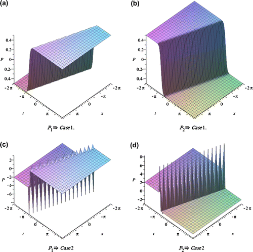
Figure 2. The Solitary wave solution of Equation (3.12).

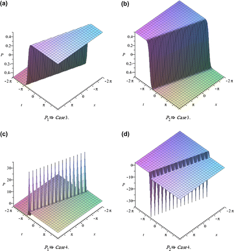
Figure 3. The Solitary wave solution of Equation (3.12).

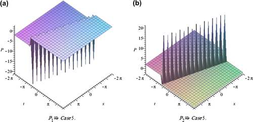
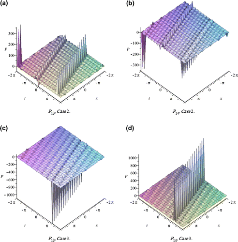
Figure 4. The Solitary wave solution of Equation (3.13).

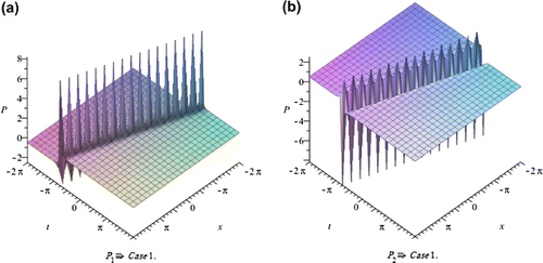
Figure 5. The Solitary wave solution of Equation (3.13).

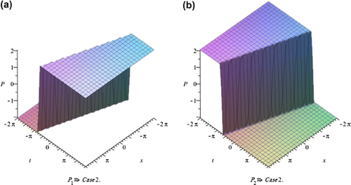
Figure 6. The Solitary wave solution of Equation (3.13).

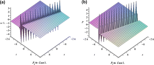
Figure 7. The Solitary wave solution of Equation (3.13).

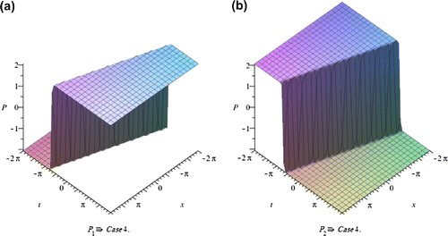
Figure 8. The Solitary wave solution of Equation (3.13).

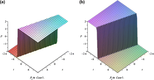
Figure 9. The Solitary wave solution of Equation (3.14).

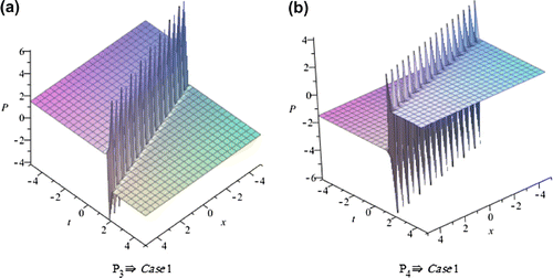
Figure 10. The Solitary wave solution of Equation (3.14).

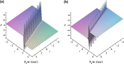
Figure 11. The Solitary wave solution of Equation (3.15).

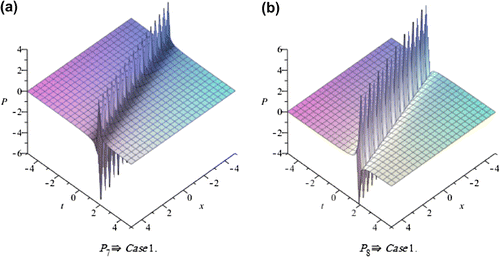
Figure 12. The Solitary wave solution of Equation (3.16).

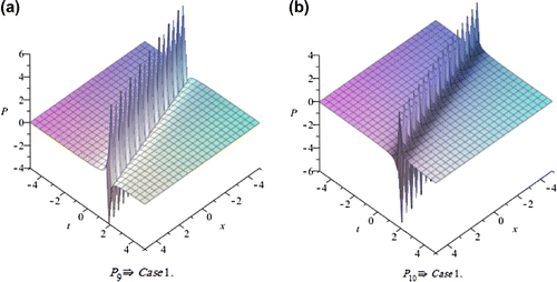
Figure 13. The Solitary wave solution of Equation (3.17).

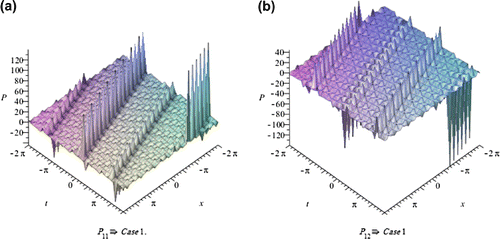
Figure 14. The Solitary wave solution of Equation (3.17).

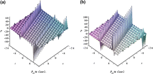
Figure 15. The Solitary wave solution of Equations (3.17 and 3.18).

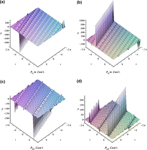
Figure 16. The Solitary wave solution of Equation (3.18).

5. Conclusion

The exp$(-\mathit{\phi }(\mathit{\xi }))$-expansion method has been applied in this paper to find the exact traveling wave solutions and then the solitary wave solutions of the generalized Hirota-Satsuma couple KdV system . Let us compare between our results obtained in the present article with the well-known results obtained by other authors using different methods as follows: our results of nonlinear dynamics of the generalized Hirota-Satsuma couple KdV system are new and different from those obtained in Yan (2003), and Figures 1–16, show the solitary traveling wave solution of the generalized Hirota-Satsuma couple KdV system . We can conclude that the exp$(-\mathit{\phi }(\mathit{\xi }))$-expansion method is a very powerful and efficient technique in finding exact solutions for wide classes of nonlinear problems and can be applied to many other nonlinear evolution equations in mathematical physics. Another possible merit is that the reliability of the method and the reduction in the size of computational domain give this method a wider applicability.

Additional information

Funding

The authors received no direct funding for this research.

Notes on contributors

Mostafa M.A. Khater

Mostafa M.A. Khater is a researcher in pure mathematics specially finding the exact and solitary wave solutions of NLPDES. He has Bsc and MSc from Zagazig University (2011) and Mansoura University(2016). He published 26 research articles in some international journals. He is a reviewer of some global journals and also editor board of Journal of Research in Applied Sciences (JRAS) and Journals of Harmonized Research.

References

- Abdelrahman, M. A. E., Zahran, E. H. M., & Khater, M. M. A. (2015). Exact traveling wave solutions for modified Liouville equation arising in mathematical physics and biology. International Journal of Computer Applications, 112(12), 0975 8887.
- Abdelrahman, M. A. E., Zahran, E. H. M., & Khater, M. M. A. (2014). Exact traveling wave solutions for power law and Kerr law non linearity using the exp-expansion method. Global Journal of Science Frontier Research, 14(4).
- Alquran, M., & Qawasmeh, A. (2014). Soliton solutions of shallow water wave equations by means of-expansion method. Journal of Applied Analysis and Computation, 4, 221–229.
- Aminikhad, H., Moosaei, H., & Hajipour, M. (2009). Exact solutions for nonlinear partial differential equations via exp-function method. Numerical Methods for Partial Differential Equations, 26, 1427–1433.
- Dai, C. Q., & Zhang, J. F. (2006). Jacobian elliptic function method for nonlinear differential difference equations. Chaos Solutions Fractals, 27, 1042–1049.
- El-Wakil, S. A., & Abdou, M. A. (2007). New exact travelling wave solutions using modified extented tanh-function method. Chaos Solitons & Fractals, 31, 840–852.
- Fan, E. (2000). Extended tanh-function method and its applications to nonlinear equations. Physics Letters A, 277, 212–218.
- Fan, E., & Zhang, H. (1998). A note on the homogeneous balance method. Physics Letters A, 246, 403–406.
- Fan, E., & Zhang, J. (2002). Applications of the Jacobi elliptic function method to special-type nonlinear equations. Physics Letters A, 305, 383–392.
- He, J. H., & Wu, X. H. (2006). Exp-function method for nonlinear wave equations. Chaos Solitons Fractals, 30, 700–708.
- Islam, R., Nur Alam, Md., Kazi Sazzad Hossain, A. K. M., Harun-Or-Roshid, & Ali Akbar, M. (2013). Traveling wave solutions of nonlinear evolution equations via exp-expansion method. Global Journal of Science Frontier Research Mathematics and Decision Sciences, 13, 63–71.
- Khater, M. M. A. (2015). On the new solitary wave solution of the generalized Hirota--Satsuma couple KdV system. Global Journal of Science Frontier Research-A, 15(4).
- Liu, S., Fu, Z., Liu, S., & Zhao, Q. (2001). Jacobi elliptic function expansion method and periodic wave solutions of nonlinear wave equations. Physics Letters A, 289, 69–74.
- Malfliet, W. (1992). Solitary wave solutions of nonlinear wave equation. American Journal of Physics, 60, 650–654.
- Malfliet, W., & Hereman, W. (1996). The tanh method: Exact solutions of nonlinear evolution and wave equations. Physica Scripta, 54, 563–568.
- Qawasmeh, A., & Alquran, M. (2014a). Reliable study of some new fifth-order nonlinear equations by means of -expansion method and rational sine--cosine method. Applied Mathematical Sciences, 8, 5985–5994.
- Qawasmeh, A., & Alquran, M. (2014b). Soliton and periodic solutions for (2+1)-dimensional dispersive long water-wave system. Applied Mathematical Sciences, 8, 2455–2463.
- Rahman, N., Nur Alam, Md., Harun-Or-Roshid, Akter, S., & Ali Akbar, M. (2014). Application of expansion method to find the exact solutions of Shorma--Tasso--Olver equation. African Journal of Mathematics and Computer Science Research, 7(1), 1–6.
- Ren, Y. J., & Zhang, H. Q. (2006). A generalized F-expansion method to find abundant families of Jacobi elliptic function solutions of the (2+1)-dimensional Nizhnik--Novikov--Veselov equation. Chaos Solitons Fractals, 27, 959–979.
- Wang, M. L. (1996). Exct solutions for a compound KdV-Burgers equation. Physics Letters A, 213, 279–287.
- Wang, M. L., Zhang, J. L., & Li, X. Z. (2008). The - expansion method and travelling wave solutions of nonlinear evolutions equations in mathematical physics. Physics Letters A, 372, 417–423.
- Wazwaz, A. M. (2004a). The tanh method for travelling wave solutions of nonlinear equations. Applied Mathematics and Computation, 154, 714–723.
- Wazwaz, A. M. (2004b). A sine--cosine method for handling nonlinear wave equations. Mathematical and Computer Modelling, 40, 499–508.
- Wazwaz, A. M. (2005). Exact solutions to the double sinh-Gordon equation by the tanh method and a variable separated ODE method. Computers & Mathematics with Applications, 50, 1685–1696.
- Yan, C. (1996). A simple transformation for nonlinear waves. Physics Letters A, 224, 77–84.
- Zahran, E. H. M., & Khater, M. M. A. (2014a). The modified simple equation method and its applications for solving some nonlinear evolutions equations in mathematical physics, Jokull Journal, 64, 297–312.
- Zahran, E. H. M., & Khater, M. M. A. (2014b). Exact solutions to some nonlinear evolution equations by the -expansion method. Jokull Journal, 64, 226–238.
- Zahran, E. H. M., & Khater, M. M. A. (2014c). Exact traveling wave solutions for the system of shallow water wave equations and modified Liouville equation using extended Jacobian elliptic function expansion method. American Journal of Computational Mathematics (AJCM), 4, 455.
- Zhang, J. L., Wang, M. L., Wang, Y. M., & Fang, Z. D. (2006). The improved F-expansion method and its applications. Physics Letters A, 350, 103–109.
- Zhang, S., Tong, J. L., & Wang, W. (2008). A generalized - expansion method for the mKdv equation with variable coefficients. Physics Letters A, 372, 2254–2257.
- Zhang, Z. Y. (2008). New exact traveling wave solutions for the nonlinear Klein--Gordon equation. Turkish Journal of Physics, 32, 235–240.
- Yan, Z. (2003). The extended Jacobian elliptic function expansion method and its application in the generalized Hirota--Satsuma coupled KdV system. Chaos, Solitons & Fractals, 15, 575–583.