Phase-I design structure of Bayesian variance chart

Abstract

This article develops a new design structure for S²-Chart, namely Bayesian variance chart, in Phase-I analysis assuming the normality of the quality characteristic to incorporate the parameter uncertainty. Our approach consists of two stages: (i) construction of the control limits for S²-Chart and (ii) performance evaluation of the proposed control limits. The comparison of the proposed design structure with the frequentist design structure of S²-Chart is examined in terms of (i) width of control region and (ii) OC curves when the process variance goes out of control. It is observed that the proposed Phase-I S²-Chart is more efficient than the frequentist S²-Chart in discriminatory power of detecting a shift in the process dispersion. When the process variance is in-control (after implementation of Bayesian variance chart), then the control limits for $\overline{X}$-Chart using in-control standard deviation are also given here for monitoring unknown mean under unknown standard deviation case.

Keywords:

• process control
• variance Chart
• posterior distribution
• OC function
• predictive limits

Public Interest Statement

The products are produced every day in industry to fulfill the requirement of the common people. The most important issue of any produced products is its quality that is the major concern of any buyer. The quality control is an important field in industrial engineering. This work helps quality engineers to meet the challenges of buyers in the market. This work gives a very useful method to control the quality of outgoing item after meeting the specification.

1. Introduction

There is a large literature on the process variability control charts. To develop a variability control chart, a basic assumption is that the underlying distribution of the quality characteristics should be normal. Here, we assume that the lot-to-lot quality (process standard) observed after a fixed time interval remains constant throughout. The constant environmental stress on the operating conditions of the process over a long period leads to an unduly restrictive and unrealistic assumption about the constant standards of the process. The situation becomes alarming when one is going for quality control of the process of the same nature accomplishing the same task in varying conditions. Obviously, for overcoming the situation, it seems logical to assume variations in process standard represented by known suitable prior distribution. More so, the process control (PC) is a continuous quality valuation process and, as such, in all PC techniques, a strong prior information representing variations in quality is available as discussed by Sharma, Singh, and Geol (2007).

Chhikara and Guttman (1982) developed a procedure for prediction limits for the inverse Gaussian distribution for both frequentists and a Bayesian viewpoint. Sharma and Bhutani (1992) extended the concept of modified classical consumer’s risk and Bayes consumer’s risk. In all these studies, the main emphasis has been to update the prior distribution with experimental data to get posterior distribution. Menzefricke (2002, 2007) developed control limits for $\overline{X}$-Chart and generalized variance chart based on posterior predictive distribution. Menzefricke (2010) developed a control chart for the variance of the normal distribution and equivalently, the coefficient of variation of a log-normal distribution. These control limits are referring to as prospective or Phase-II control limits because these limits are based on the future outcome (predictive inference) of the process. Sharma et al. (2007) discussed the performance of $\overline{X}$-Chart and R-Chart when standards vary randomly using OC function and ARL as performance measures. Saghir (2007) evaluated the performance of $\overline{X}$-Chart and S-Chart when standards vary randomly based on power function as performance measure. Recently, Saghir (2015) proposed a Phase-I control limits of $\overline{X}$-Chart based on posterior distribution of the statistic to monitor the mean of normal distribution. He concluded that when the process mean is statistically in-control for Phase-I samples based on these Bayesian limits, the Phase-II monitoring of the sample mean using Menzefricke (2002) control limits could be used.

This study proposes a new design structure for variance control chart namely S²-Chart based on Bayesian approach for monitoring the Phase-I data following Menzefricke (2002, 2007, 2010), Chen, Morris, and Martin (2005), and Saghir (2007, 2015). The performance evaluation of S²-Chart has been studied following Chhikara and Guttman (1982) and Saghir (2007, 2015). The rest of the article is summarized as follows. In Section 2, the control limits of S²-Chart for Phase-I analysis based on posterior distribution for informative and non-informative priors are constructed. In Section 3, the evaluation performance of the constructed control limits is made. In Section 4, the comparison between the Bayesian variance chart and the frequentist S²-Chart for Phase-I analysis is made through simulation. Section 5 developed the design structure of $\overline{X}$-Chart for simultaneous monitoring of process mean and standard deviation. Section 6 offers some concluding remarks and recommendations for further study. The necessary derivations of the distribution used in this study are provided in Appendix A.

2. The proposed design structure

The Phase-I design structure of S²-Chart based on posterior distribution for monitoring process variation assuming the parameter uncertainty following Woodall and Montgomery (1999), Menzefricke (2002, 2007, 2010), and Saghir (2007, 2015) will be proposed in this section. In the following subsections, the control limits of S²-Chart, using (i) informative prior and (ii) non-informative prior distributions, are constructed.

2.1. Construction of the control limits based on informative prior

Let x₁, x₂, …, x_n be a random sample of size n drawn from normal distribution with unknown mean μ and unknown variance σ². The probability density function and the likelihood function of random variable X are defined, respectively, as:(1) $$f(X\left|\mathit{\mu },{\mathit{\sigma }}^2\right.)=\frac{1}{\sqrt{2\mathit{\pi }}\mathit{\sigma }}{e}^{-\frac{1}{2{\mathit{\sigma }}^2}{\left(x_i-\mathit{\mu }\right)}^2};-\infty <x_i<\infty ,\mathit{\sigma }>0.$$(1)

and(2) $$L(X\left|\mathit{\mu },{\mathit{\sigma }}^2\right.)=\prod _{i=1}^{n}f(x_i\left|\mathit{\mu },{\mathit{\sigma }}^2)\right.$$(2)

There are two sources of information regarding unknown mean μ and variance σ², the prior information and results from a calibration sample, which help update the information about unknown parameters. The parameter μ has simple family of conjugate prior distribution (normal distribution). The parameter σ² does not have any simple family of conjugate prior distributions because its marginal likelihood depends in a complex way on the data (see Hill, 1965; Tiao & Tan, 1965). However, the inverse-gamma family is conditionally conjugate for σ² (Gelman, 2006). This conditionally conjugacy allows σ² to be updated easily using the Gibbs sampler (Gelfand & Smith, 1990) and also allows the prior distribution to be interpreted in terms of equivalent data (see Box & Tiao, 1973).

The usual priors used for unknown mean and precision (see Menzefricke, 2002, 2010) are:

(3) $$\left.\begin{array}{c}p(\left.\mathit{\mu }\right|{\mathit{\sigma }}^2)=N\left(m_0,\frac{{\mathit{\sigma }}^2}{n_0}\right)\\ p({\mathit{\sigma }}^{-2})=Ga\left(\frac{v_0}{2},\frac{v_0}{2}{S}_0^2\right)\\ \end{array}\right\},$$(3)

where “N” and “Ga” denote normal and gamma distributions, respectively, and $\left\{m_0,\frac{{\mathit{\sigma }}^2}{n_0}\right\}$, $\left\{\frac{v_0}{2},\frac{v_0}{2}{S}_0^2\right\}$ are hyper-parameters of the prior distributions as defined in Menzefricke (2002) and similar to hyper-parameter $\{1,{\mathit{\sigma }}_x^{-2}\}$used for unknown precision, r, of Gaussian mixture model in Chen et al. (2005).

The prior distribution for variance can be derived from precision distribution as;(4) $$p\left({\mathit{\sigma }}^2\right)=\frac{{\left(\frac{v_0}{2}{S}_0^2\right)}^{\frac{v_0}{2}}}{\mathrm{\Gamma }\frac{v_0}{2}}{\left(\frac{1}{{\mathit{\sigma }}^2}\right)}^{\frac{v_0}{2}+1}{e}^{-\frac{{\left(\frac{v_0}{2}{S}_0\right)}^2}{{\mathit{\sigma }}^2}};0<{\mathit{\sigma }}^2<\infty$$(4)

This density is known as inverse-gamma distribution as discussed in Bernardo and Smith (2004, p. 119), Spiegelhalter, Thomas, Best, Gilks, and Lunn (1994/2003) and Gelman (2006). Therefore, the prior for unknown mean and variance becomes:

(5) $$\left.\begin{array}{c}p(\left.\mathit{\mu }\right|{\mathit{\sigma }}^2)=N\left(m_0,\frac{{\mathit{\sigma }}^2}{n_0}\right)\\ p({\mathit{\sigma }}^2)=IG\left(\frac{v_0}{2},\frac{v_0}{2}{S}_0^2\right)\\ \end{array}\right\}$$(5)

If the data x₁, x₂, …, x_n are from stable process, the sufficient statistics are the sample mean $\overline{x}={\sum }_{i=1}^n{x}_i/n$ and variance $S_x^2={\sum }_{i=1}^n{(x_i-\overline{x})}^2/(n-1)$ for a calibration sample of size n (see Menzefricke, 2010). The joint distribution of sample mean and variance, i.e. $f(\overline{x},s_x^2\left|\mathit{\mu },{\mathit{\sigma }}^2)\right.$, is thus:

(6) $$f(\overline{x},s_x^2\left|\mathit{\mu },{\mathit{\sigma }}^2)=f(\overline{x}\left|\mathit{\mu },{\mathit{\sigma }}^2)f(s_x^2\left|{\mathit{\sigma }}^2\right.)\right.\right.$$(6)

where $f(\overline{x}|\mathit{\mu },{\mathit{\sigma }}^2)=N\left(\mathit{\mu },\frac{{\mathit{\sigma }}^2}{n}\right)$ and $f(s_x^2\left|{\mathit{\sigma }}^2\right.)=Ga\left(\frac{n-1}{2},\frac{n-1}{2{\mathit{\sigma }}^2}\right)$ as defined in Menzefricke (2002, 2010).

Following the methodology of Aitchison and Dunsmore (1975), the posterior distribution of f(μ, σ²) given $(\overline{x},s_x^2)$ is:(7) $$p(\mathit{\mu },{\mathit{\sigma }}^2\left|\overline{x},S_x^2\right.)=\frac{\sqrt{n_c}}{\mathit{\sigma }\sqrt{2\mathit{\pi }}}{e}^{-\frac{n_c}{2{\mathit{\sigma }}^2}{(\mathit{\mu }-m_1)}^2}{\left(\frac{\mathit{\beta }}{\mathit{\Gamma }\mathit{\alpha }}\right)}^{\mathit{\alpha }}{\left(\frac{1}{{\mathit{\sigma }}^2}\right)}^{\mathit{\alpha }+1}{e}^{-\left(\frac{\mathit{\beta }}{{\mathit{\sigma }}^2}\right)}-\infty <\mathit{\mu }<\infty ,0<{\mathit{\sigma }}^2<\infty .=p(\mathit{\mu }\left|\overline{x},{\mathit{\sigma }}^2)p({\mathit{\sigma }}^2\left|s_x^2)\right.\right.$$(7)

The derivation of (7) is given in Appendix A. The random variable $\mathit{\mu }\left|(\overline{x}\right.,{\mathit{\sigma }}^2)$ is normally distributed random variable with mean $E(\mathit{\mu }\left|(\overline{x},{\mathit{\sigma }}^2)\right.)=m_1$ (posterior mean) and variance $V(\mathit{\mu }\left|(\overline{x},{\mathit{\sigma }}^2)\right.)=\frac{{\mathit{\sigma }}^2}{n_c}$ (posterior variance); ${\mathit{\sigma }}^2\left|S_x^2\right.$ is inverse-gamma distributed random variable with parameters $\mathit{\alpha }=\frac{v_1}{2}$, β =  $\left(\frac{v_0}{2}{S}_0^2+\frac{n-1}{2}{s}_x^2+\frac{n_{0}n}{n_0+n}{(m_0-\overline{x})}^2\right)$ and the values of v₁, m₁, and n_c are defined in Appendix A.

The lower control limit, central line, and upper control limit are the three parameters of a Shewhart-type control chart. Assuming the measurable quality characteristic, X, to be normally distributed with unknown mean μ and unknown variance σ², the control limits for the usual S²-Chart for retrospective analysis are defined as:

(8) $$\left.\begin{array}{c}LCL=\frac{\overline{S_x^2}}{n-1}{\mathit{\chi }}_{(1-\frac{\mathit{\alpha }}{2})}^2\\ CL=\overline{S_x^2}\\ UCL=\frac{\overline{S_x^2}}{n-1}{\mathit{\chi }}_{(\frac{\mathit{\alpha }}{2})}^2\\ \end{array}\right\},$$(8)

where α is the level of significance or false alarm rate in quality terminology, $\overline{S_x^2}$is the average of variance of k-subgroups each of size n, ${\mathit{\chi }}_{{}_{(1-\frac{\mathit{\alpha }}{2})}}^2$and ${\mathit{\chi }}_{{}_{(\frac{\mathit{\alpha }}{2})}}^2$ are the quantile points of the chi-square distribution as defined in Montgomery (2004, p. 249).

Now in a situation where variations in process variance σ² are assumed to be represented by a prior distribution given in (5) and using the sample information variation, the process variance can be updated in the form of posterior distribution as given in (7). The usual three-sigma control limits, for S²-Chart using the updated posterior distribution, are given by:(9) $$\begin{array}{c}LCL=\frac{\mathit{\beta }}{\mathit{\alpha }-1}-3\frac{\mathit{\beta }}{(\mathit{\alpha }-1){(\mathit{\alpha }-2)}^{\frac{1}{2}}}\\ CL=\frac{\mathit{\beta }}{\mathit{\alpha }-1}\\ UCL=\frac{\mathit{\beta }}{\mathit{\alpha }-1}+3\frac{\mathit{\beta }}{(\mathit{\alpha }-1){(\mathit{\alpha }-2)}^{\frac{1}{2}}}\\ \end{array}$$(9)

where the parameters $\mathit{\alpha }=\frac{v_1}{2}$, β =  $\left(\frac{v_0}{2}{S}_0^2+\frac{n-1}{2}{s}_x^2+\frac{n_{0}n}{n_0+n}{(m_0-\overline{x})}^2\right)$ and the values of v₁, m₁, and n_c are defined in Appendix A.

The distribution of sufficient statistic $S_x^2$ is not a symmetric even for moderate to large samples. Therefore, the true probability limits for S²-Chart using posterior distribution following Chhikara and Guttman (1982) are given by:(10) $$\left.\begin{array}{c}\underset{-\infty }{\overset{LCL}{\int }}p({\mathit{\sigma }}^2\left|S_x^2)\right.d{\mathit{\sigma }}^2=\frac{\mathit{\alpha }}{2}\\ \underset{UCL}{\overset{\infty }{\int }}p({\mathit{\sigma }}^2\left|S_x^2)\right.d{\mathit{\sigma }}^2=\frac{\mathit{\alpha }}{2}\\ \end{array}\right\},$$(10)

where $p({\mathit{\sigma }}^2\left|S_x^2)\right.$ is as given in (7) and α is the level of significance, which is 0.0027 in Shewhart-type control charts. We are updating the control limits of S²-Chart for monitoring the unknown process variance. So, the plotted statistic is the sample variance $S_x^2$ because it is an unbiased estimator of σ² which is a variable of interest.

2.2. Control limits for $\overline{X}$-Chart based on non-informative prior

In this subsection, we have proposed control limits for S²-Chart based on non-informative prior distribution. We have considered uniform prior and Jeffrey’s prior as non-informative prior.

2.2.1. Control limits based on Jeffrey’s prior

In this subsection, we have proposed control limits for S²-Chart based on Jeffrey’s prior for unknown mean and variance of the normal distribution, so that we are then relying primarily on the likelihood involved for our inference following the work of Box (1980), Chhikara and Guttman (1982), and Gelman (2006).

Consider the sampling distribution of X, likelihood function of X, and sampling distribution of ($\overline{X}$, S²) as defined in Equations (1), (2), and (6). The Jeffrey’s prior for unknown mean and variance as discussed in Banerjee and Bhattacharyya (1979) and Gelman (2006) is:(11) $$p(\mathit{\mu },{\mathit{\sigma }}^2)\infty {\mathit{\sigma }}^{-}2-\infty <\mathit{\mu }<\infty ,0<{\mathit{\sigma }}^2<\infty .$$(11)

where σ⁻² is the precision of normal distribution. Then, following the methodology of Menzefricke (2002, 2007, 2010), the posterior distribution of f(μ, σ²) given $(\overline{x},s_x^2)$is defined as:(12) $$p(\mathit{\mu },{\mathit{\sigma }}^2\left|\overline{x},S_x^2\right.)=\frac{\sqrt{n}}{\mathit{\sigma }\sqrt{2\mathit{\pi }}}{e}^{-\frac{n}{2{\mathit{\sigma }}^2}{(\mathit{\mu }-\overline{x})}^2}{\left(\frac{\mathit{\beta }}{\mathit{\Gamma }\mathit{\alpha }}\right)}^{\mathit{\alpha }}{\left(\frac{1}{{\mathit{\sigma }}^2}\right)}^{\mathit{\alpha }+1}{e}^{-\left(\frac{\mathit{\beta }}{{\mathit{\sigma }}^2}\right)};-\infty <\mathit{\mu }<\infty ,0<{\mathit{\sigma }}^2<\infty .=p(\mathit{\mu }\left|\overline{x},{\mathit{\sigma }}^2)p({\mathit{\sigma }}^2\left|s_x^2)\right.\right.$$(12)

where $\mathit{\mu }\left|(\overline{x}\right.,{\mathit{\sigma }}^2)$ is normally distributed random variable with mean $E(\mathit{\mu }\left|(\overline{x},{\mathit{\sigma }}^2)\right.)=\overline{x}$ and variance$V(\mathit{\mu }\left|(\overline{x},{\mathit{\sigma }}^2)\right.)=\frac{{\mathit{\sigma }}^2}{n}$; ${\mathit{\sigma }}^2\left|S_x^2\right.$ is inverse-gamma distributed random variable with parameters$\mathit{\alpha }=\frac{n-1}{2}$, $\mathit{\beta }=(\frac{n-1}{2}{S}_x^2)$. The derivation of (12) is given in Appendix A.

Now in a situation where variation in process variance σ² is assumed to be represented by a prior distribution given in (11) and using the sample information variation, the process variance can be updated in the form of posterior distribution as given in (12). The true probability control limits for S²-Chart using posterior distribution using Jeffrey’s non-informative prior are given by:(13) $$\left.\begin{array}{c}\underset{-\infty }{\overset{LCL}{\int }}p({\mathit{\sigma }}^2\left|S_x^2)\right.d{\mathit{\sigma }}^2=\frac{\mathit{\alpha }}{2}\\ \underset{UCL}{\overset{\infty }{\int }}p({\mathit{\sigma }}^2\left|S_x^2)\right.d{\mathit{\sigma }}^2=\frac{\mathit{\alpha }}{2}\\ \end{array}\right\},$$(13)

where $p({\mathit{\sigma }}^2\left|S_x^2)\right.$ is as given in (12) and α is the level of significance, which is 0.0027 in Shewhart-type control charts.

2.2.2. Control limits based on uniform prior

In this subsection, we have proposed control limits for S²-Chart based on uniform prior distribution for unknown mean and variance of the normal distribution, so that we are then relying primarily on the likelihood involved for our inference following the work of Box (1980), Chhikara and Guttman (1982), and Gelman (2006).

The uniform prior for unknown mean and variance is p(μ, σ²)∞1. The posterior distribution of f(μ, σ²) given $(\overline{x},s_x^2)$is defined as:(14) $$p(\mathit{\mu },{\mathit{\sigma }}^2\left|\overline{x},S_x^2\right.)=\frac{n}{\mathit{\sigma }\sqrt{2\mathit{\pi }}}{e}^{-\frac{n}{2{\mathit{\sigma }}^2}{(\mathit{\mu }-\overline{x})}^2}{\left(\frac{\mathit{\beta }}{\mathit{\Gamma }\mathit{\alpha }}\right)}^{\mathit{\alpha }}{\left(\frac{1}{{\mathit{\sigma }}^2}\right)}^{\mathit{\alpha }+1}{e}^{-\left(\frac{\mathit{\beta }}{{\mathit{\sigma }}^2}\right)}-\infty <\mathit{\mu }<\infty ,0<{\mathit{\sigma }}^2<\infty .=p(\mathit{\mu }\left|\overline{x},{\mathit{\sigma }}^2)p({\mathit{\sigma }}^2\left|s_x^2)\right.\right.$$(14)

where $\mathit{\mu }\left|(\overline{x}\right.,{\mathit{\sigma }}^2)$ is normally distributed random variable with mean $E(\mathit{\mu }\left|(\overline{x},{\mathit{\sigma }}^2)\right.)=\overline{x}$ and variance $V(\mathit{\mu }\left|(\overline{x},{\mathit{\sigma }}^2)\right.)=\frac{{\mathit{\sigma }}^2}{n}$; ${\mathit{\sigma }}^2\left|S_x^2\right.$ is inverse-gamma distributed random variable with parameters $\mathit{\alpha }=\frac{n-3}{2}$,$\mathit{\beta }=(\frac{n-1}{2}{S}_x^2)$.

The control limits for S²-Chart using Bayesian inference following Chhikara and Guttman (1982) based on uniform prior distribution are given by:

(15) $$\left.\begin{array}{c}\underset{-\infty }{\overset{LCL}{\int }}p({\mathit{\sigma }}^2\left|S_x^2)\right.d{\mathit{\sigma }}^2=\frac{\mathit{\alpha }}{2}\\ \underset{UCL}{\overset{\infty }{\int }}p({\mathit{\sigma }}^2\left|S_x^2)\right.d{\mathit{\sigma }}^2=\frac{\mathit{\alpha }}{2}\\ \end{array}\right\},$$(15)

where $p({\mathit{\sigma }}^2\left|S_x^2)\right.$ is as given in (14) and α is the level of significance, which is 0.0027 in Shewhart-type control charts.

The limits defined in Equations (10), (13), and (15) are based on updated information and can be used to monitor the unknown normal process variance. The successive sample of a given size n are observed if a sample variance is outside the control limits defined in Equations (10), (13), and (15) chart signals. If a sample variance or more sample variances falls outside the control limits, the trial control limits will be revised until all the sample variances lie within the control region. When the process is in-control, the future sample variances are generated from the posterior predictive distribution as proposed by Menzefricke (2010); otherwise, the use of these will be misleading as discussed by many authors including Montgomery (2004) and Saghir (2015). This work is related to the Phase-I monitoring of S²-Chart while the work of Menzefricke (2010) is for Phase-II monitoring. The Phase-I monitoring is necessary before applying the Phase-II study, see Montgomery (Box, 1980).

3. Evaluation of control limits

For the evaluation of the control limits obtained by frequentist (sampling) and Bayesian methods, we use OC function under the hypothetical situation that the variance of the normal distribution does not remain at level σ² following Sharma et al. (2007), Saghir (2007), and Menzefricke (2010). At this stage, we use sampling theoretical considerations approach following Menzefricke, (2002, 2007, 2010) and Saghir (2007, 2015). Let the sampling distribution for the next sample variance be $IG(\mathit{\alpha },\frac{\mathit{\beta }}{{\mathit{\alpha }}_2{\mathit{\beta }}_0^2})$ where α₂ is an amount of shift in the process variance ${\mathit{\sigma }}_0^2$.

The OC function in the corresponding situations provides a measure of the sensitivity of the control limits, i.e. their ability to detect a shift in the mean of the process quality characteristic following Menzefricke (2002, 2010) and Sharma et al. (2007). The relative distribution of ${\mathit{\sigma }}^2\left|S_x^2\right.$ to shifted variance ${\mathit{\alpha }}_2{\mathit{\sigma }}_0^2$ is derived in Appendix A. The OC function for S²-Chart based on the control limits defined in (10) and relative distribution is defined as:(16) $$\begin{array}{c}{B}_I=\text{Pr}[\text{not detecting a shift in the variance of data generating process (using informative prior) on the first sample following the shift}]\\ =\text{Pr}[LCL\le {\mathit{\sigma }}_0^2\le UCL|{\mathit{\alpha }}_2{\mathit{\sigma }}_0^2]\\ =\underset{LCL}{\overset{UCL}{\int }}{\mathit{\alpha }}_2{\mathit{\sigma }}_0^2*IG(\mathit{\alpha },\frac{\mathit{\beta }}{{\mathit{\alpha }}_2{\mathit{\sigma }}_0^2})d{\mathit{\sigma }}^2\\ \end{array}$$(16)

where$\mathit{\alpha }=\frac{v_1}{2}$, β = $(\frac{v_0}{2}{S}_0^2+\frac{n-1}{2}{S}_x^2+\frac{n_{0}n}{n_0+n}{(m_0-\overline{x})}^2)$ and “IG” denotes inverse-gamma distribution and a₂ denotes the amount of shift in variance ${\mathit{\sigma }}_0^2$.

The OC function for S²-Chart based on the control limits defined in Equation (13) and relative distribution is defined as:(17) $$\begin{array}{c}{B}_{JNI}=\text{Pr}[\text{not detecting a shift in the variance of data generating process}({\text{using Jeffrey}}^{\prime }\text{s}\text{non-informative prior})\text{on the first sample following the shift}]\\ =\text{Pr}[LCL\le S_x^2\le UCL|{\mathit{\alpha }}_2{\mathit{\sigma }}_0^2]\\ B_{JNI}=\underset{LCL}{\overset{UCL}{\int }}IG(\frac{n-1}{2},\frac{(n-1)S_x^2}{2{\mathit{\alpha }}_2{\mathit{\sigma }}_0^2})d{\mathit{\sigma }}^2\\ \end{array}$$(17)

The OC function for S²-Chart based on the control limits defined in Equation (15) and relative distribution is defined as:(18) $$\begin{array}{c}{B}_{UNI}=\text{Pr}[\text{not detecting a shift in the variance of data generating process (using Uniform non- informative prior) on the first sample following the shift}]\\ =\text{Pr}[LCL\le S_x^2\le UCL|{\mathit{\alpha }}_2{\mathit{\sigma }}_0^2]\\ B_{UNI}=\underset{LCL}{\overset{UCL}{\int }}IG(\frac{n-3}{2},\frac{(n-1)S_x^2}{2{\mathit{\alpha }}_2{\mathit{\sigma }}_0^2})d{\mathit{\sigma }}^2\\ \end{array}$$(18)

The corresponding OC function for usual control limits of S²-Chart is:(19) $$\begin{array}{c}{B}_F=\text{Pr}[\text{not detecting a shift in the variance of data generating process on the first sample following the shift}]\\ =\text{Pr}\left[LCL\right.\le S_x^2\le UC{L}_{}\left.\left|a_2^{}{\mathit{\sigma }}_0^2\right.\right]\\ {\int }_{LCL}^{UCL}Ga(\frac{n-1}{2},\frac{n-1}{2a_2^{}{\mathit{\sigma }}_0^2})d{S}_x^2.\\ \end{array}$$(19)

where “Ga” denotes gamma distribution with parameters $\frac{n-1}{2}$ and $\frac{n-1}{2a_2^{}{\mathit{\sigma }}_0^2}$.

4. Simulation study and comparison

In this section, we have made a comparison among the proposed (informative and non-informative) control limits and usual control limits of S²-Chart. First, we have made comparison based on control region obtained by the proposed and usual limits following Chhikara and Guttman (Sharma et al., 2007) and then the comparison based on OC $S_x^2$ function following Menzefricke (2002, 2007, 2010), Sharma et al. (2007), and Saghir (2007, 2015) is provided.

4.1. Control region-based comparison

In this subsection, a comparison of the proposed limits with the frequentist control limits of S²-Chart for the initials samples is made. The comparison based on width of the control limits is made for Phase-I process monitoring. Using Monte Carlo simulation technique, 10,000 random samples are drawn from standard normal process of size nine and sample variance along standard error is calculated and given in Tables 1–3. Let us assume that (i) α = 0.0027 and (ii) $\overline{\overline{x}}=m_0$ (without loss of generality). We have considered three situations when (i) $S_x^2=S_0^2$, (ii) $S_x^2<S_0^2$, and (iii) $S_x^2>S_0^2$. The critical region defined in Equation (10) changes with the posterior degree of freedom v₁ which is a measure of the amount of uncertainty regarding the unknown process variance, σ² (see Menzefricke, 2002, 2010). The control limits v₁for S²-Chart for different values of v₁ based on these random samples and updated posterior distribution are calculated and given here in Tables 1–3 for comparison purposes.

Table 1. Control limits of S²-Chart for $S_x^2$ = 0.92884 (0.0034) and $S_0^2$ = 0.92884

Control limits of S^2-Chart		(LCL, UCL)	Width
Frequentist		(0.13100, 2.73710)	2.60610
IN prior based	v1 = 10	(0.34524, 4.98952)	4.64428
	v1 = 15	(0.37851, 3.80397)	3.42546
	v1 = 20	(0.41885, 3.01139)	2.59254
	v1 = 40	(0.51452, 2.02075)	1.50623
JNI prior based		(0.29299, 7.89839)	7.60540
UNI prior based		(0.34179, 17.54890)	17.20711

Table 2. Control limits of S²-Chart for $S_x^2$ = 0.92884 (S.E = 0.0034), $S_0^2$ = 0.5000

Control limits of S^2-Chart		(LCL, UCL)	Width
Frequentist		(0.13100, 2.73710)	2.60610
IN prior based	v1 = 10	(0.29289, 5.32285)	5.02996
	v1 = 15	(0.29696, 2.98429)	2.68733
	v1 = 20	(0.30282, 2.17721)	1.87439
	v1 = 40	(0.32448, 1.27438)	0.94990
JNI prior based		(0.29299, 7.89839)	7.60540
UNI prior based		(0.34179, 17.54890)	17.20711

Table 3. Control limits of S²-Chart for $S_x^2$ = 0.92884 (S.E = 0.0034), $S_0^2$ = 1.5000

Control limits of S^2-Chart		(LCL, UCL)	Width
Frequentist		(0.13100, 2.73710)	2.60610
IN prior based	v1 = 10	(0.36234, 6.58564)	6.22330
	v1 = 15	(0.48714, 4.89559)	4.40845
	v1 = 20	(0.57338, 4.12246)	3.54908
	v1 = 40	(0.76764, 3.01483)	2.24719
JNI prior based		(0.29299, 7.89839)	7.60540
UNI prior based		(0.34179, 17.54890)	17.20711

Tables 1–3 give the following considerable points:

(1)	The width of the control region for the proposed limits decreases as posterior degree of freedom v1 increases (see last column of Tables 1–3).
(2)	Comparison across the informative prior distribution-based limits reveals that the control limits are more contract in terms of minimum width of the control region when $S_x^2$ = $S_0^2$ than other choices (see Tables 1–3).
(3)	The control limits obtained by non-informative prior distributions, which do not incorporate the parameter uncertainty (Menzefricke, 2002, 2010), are wider than frequentist control limits (see first and last two rows of Tables 1–3).
(4)	As the posterior degree of freedom v1 (which is a quantitative assessment of how much certain we are about the accuracy of the prior variance “$S_0^2$”, prior estimate of σ2, lower the variance, more accurate our believe) increases, the width of the control limits obtained based on informative prior distribution decreases.

4.2. OC curve comparison

In this subsection, we evaluate the proposed control limits of S² -Chart using OC curve as performance measures. Using the control limits, calculated in Section 4.1, OC function is calculated for different amounts of shifts (i.e. different values of α₂), α = 0.0027, n = 9, and OC curves are made and provided here in Figures 1–3.

Figure 1. OC curve for S²-Chart at $S_x^2$ = $S_0^2$ = 0.92884.

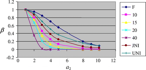
Figure 2. OC curve for S²-Chart at $S_0^2$ = 0.50000 and $S_x^2$ = 0.92884.

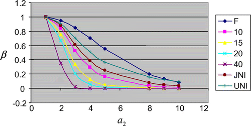
Figure 3. OC curve for S²-Chart at $S_0^2$ = 1.50000 and $S_x^2$ = 0.92884.

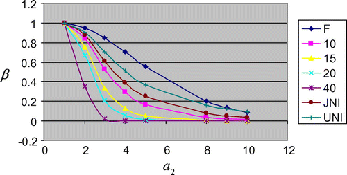
where “F” denotes OC function based on usual control limits, “JNI” OC function based on Jeffrey’s non-informative prior distribution limits, “UNI” OC function based on uniform non-informative prior distribution limits, and “10, 15, 20, 40” based on informative prior distribution degrees of freedom limits.

From Figures 1–3, it is obvious that the proposed control limits based on informative prior distribution perform better than the frequentist control limits of S²-Chart in the sense that the discriminatory power of detecting a shift in the parameter of interest is high for proposed control limits than the existing control limits of S²-Chart. The higher power of detecting a shift results in low value of OC function; therefore, the curve of OC function for the proposed control limits is less than the frequentist control limits as it is clear from Figures 1–3.

The performance of non-informative priors-based control limits of S²-Chart to detect a shift in the parameter is also better than the frequentist control limits as it is obvious from above figures but less than informative prior-based control limits’ performance. Therefore, control limits of S²-Chart based on informative prior perform better to detect a shift in a parameter of the continuous process for larger value of posterior degree of freedom v₁. The more the posterior degree of freedom v₁, more the power of detecting a shift for informative prior distribution limits, as it can be seen from Figures 1–3. A similar behavior has been observed for other choices of sample sizes and in-control false alarm rate α.

5. Control limits for $\overline{X}$-Chart when variance is unknown

In this section, we are constructing and evaluating the control limits of Bayesian $\overline{X}$-Chart based on posterior distribution for Phase-I process monitoring following Saghir (2015).

5.1. Construction of the limits

The control limits for Bayesian $\overline{X}$-Chart, based on the updated posterior distribution defined in Equation (7), when process mean as well as process variance is unknown, are:(20) $$\begin{array}{c}LC{L}_B=\frac{n_0{m}_0+n\overline{x}}{n+n_0}-Z_{\left(\frac{\mathit{\alpha }}{2}\right)}\frac{\mathit{\sigma }}{\sqrt{n+n_0}}\\ CL=\frac{n_0{m}_0+n\overline{x}}{n+n_0}\\ UC{L}_B=\frac{n_0{m}_0+n\overline{x}}{n+n_0}+Z_{\left(\frac{\mathit{\alpha }}{2}\right)}\frac{\mathit{\sigma }}{\sqrt{n+n_0}},\\ \end{array}$$(20)

where Z_(α/2) is a (α/2)th quantile point of the standard normal distribution. For the usual choice of in-control probability of false alarm rate α = 0.0027, Z_(α/2)= 3.00 and control limits defined in Equation (20) are know as 3σ-control limits. As the process standard deviation or variance is unknown, therefore, we replace unknown standard deviation by any unbiased estimator like $\widehat{\mathit{\sigma }}=\frac{\overline{R}}{d_2}$ or $\widehat{\mathit{\sigma }}=\frac{\overline{S}}{c_4}$ given in many textbooks including Montgomery (2004). We are updating the control limits of $\overline{X}$-Chart for monitoring the unknown process mean. So, the plotted statistic is the sample average $\overline{X}$ because it is an unbiased estimator of unknown population mean μ, which is the variable of interest to be monitored.

5.2. Evaluation of the limits

For the evaluation of the proposed control limits of $\overline{X}$-Chart, we have used OC function as performance measures under the hypothetical situation that the mean of the normal distribution does not remain at level μ following Saghir (2007, 2015). Let the sampling distribution for the next sample mean be $N(M,\frac{{\mathit{\sigma }}^2}{n}$) where M is the value of the in-control or out-of-control process mean and the process standard deviation is in-control at $\widehat{\mathit{\sigma }}=\frac{\overline{R}}{d_2}$ or $\widehat{\mathit{\sigma }}=\frac{\overline{S}}{c_4}$. The OC function in the corresponding situations provides a measure of the sensitivity of the control limits, i.e. their ability to not detect a shift in the mean of the process quality characteristic following Menzefricke (2002, 2007, 2010), Saghir (2007), and Saghir (2015). The OC function for $\overline{X}$-Chart based on the control limits defined in (20) is defined as:(21) $$\begin{array}{c}{B}_{I}N=Pr[notdetectingashiftinthesamplemean(usinginformativePrior)onthefirstsamplefollowingtheshift]\\ Pr[LC{L}_B\le \overline{X}\le UC{L}_B|M]\\ \mathit{\varphi }\left(\frac{UC{L}_B-M}{\widehat{\mathit{\sigma }}/\sqrt{n}}\right)-\mathit{\varphi }(\frac{LC{L}_B-M}{\widehat{\mathit{\sigma }}/\sqrt{n}})\\ \end{array}$$(21)

Let us assume that (i) M = m₀ + b where b is an amount of shift occurring in the in-control mean m₀, (ii) α = 0.0027, (iii) $\widehat{\mathit{\sigma }}=1$ (without loss of generality), and the posterior mean of μ, m₁ to be equal m_0; then, Equation (21) reduces to(22) $$B_{I}N=\mathit{\varphi }\left(-b\sqrt{n}+3\sqrt{\frac{n}{n+n_0}}\right)-\mathit{\varphi }\left(-b\sqrt{n}-3\sqrt{\frac{n}{n+n_0}}\right)$$(22)

For the given values of b and n, the OC function decreases with prior sample size n₀ and approaches 0 as n₀ → ∞. A larger value of n₀ implies more precise knowledge about m₀ and produces thus a narrower control region.

6. Conclusions and recommendations

The proposed posterior distribution-based design structure of S²-Chart, which incorporates the parameter uncertainty by considering a suitable prior distribution of unknown parameter, is more efficient than the frequentist design structure, which ignores this uncertainty and assumes that σ² = S², with reference to the width of the limits, lowest type-I error, and more power of detecting a shift in the parameter. Larger values of posterior degree of freedom v₁ provided more efficient control limits in terms of lowest width of control region as well as more discriminatory power of detecting a shift in the parameter when actually the shift occurs in the parameter. The control limits of S²-Chart based on informative prior are more efficient than non-informative prior-based control limits and usual control limits. The performance of the usual control limits is least among the compared control limits. These control limits must be calculated for Phase-I data and when the process variance is statistically in-control, the control limits proposed by Menzefricke (2010) should be used. The control limits of $\overline{X}$-Chart are also constructed when mean and standard deviation of the normal process are unknown. The constructed control limits are evaluated and it has been observed that a larger value of n₀ implies more precise knowledge about m₀. When the process mean is statistically in-control for Phase-I samples based on these Bayesian limits, the Phase-II monitoring of the sample mean using Menzefricke (2002) control limits could be used.

Additional information

Funding

Funding. The author received no direct funding for this research.

Notes on contributors

Aamir Saghir

Aamir Saghir obtained his PhD degree in Statistics from the Department of Mathematics, Zhejiang University, Hangzhou, China, under CSC program. He is currently working in Mirpur University of Science and Technology (MUST), Mirpur, Pakistan, as a senior lecturer. His research interests include Statistical Quality Control, Mathematical Statistics, and Applied Statistics.

Appendix A

In this Appendix, we have given the derivation of the distributions used in the development and comparison of the proposed Bayesian control limits of S²-Chart.

(1)	Posterior distribution of ${\mathit{\sigma }}^2\left|S_x^2\right.$ based on informative prior

The sampling distribution of sufficient statistics $\overline{x}$and S², Menzefricke (2002, 2010) is:$$\begin{array}{c}f(\overline{x}\left|\mathit{\mu },{\mathit{\sigma }}^2\right.)=N(\mathit{\mu },\frac{{\mathit{\sigma }}^2}{n}),-\infty <\overline{x}<\infty .\hfill \\ f(s_x^2\left|{\mathit{\sigma }}^2\right.)=Ga(\frac{n-1}{2},\frac{n-1}{2{\mathit{\sigma }}^2}),0<S^2<\infty .\hfill \end{array}$$

The prior distributions of μ and σ² are defined in Equation (15), so the posterior distribution of μ and σ² given that $\overline{x}$and S² will be:(1.1) $$p(\mathit{\mu },{\mathit{\sigma }}^2\left|\overline{x},S_x^2\right.)\infty p(\overline{x},S_x^2\left|\mathit{\mu },{\mathit{\sigma }}^2)p(\mathit{\mu }\left|{\mathit{\sigma }}^2)\right.p({\mathit{\sigma }}^2)\right.\Rightarrow p(\mathit{\mu },{\mathit{\sigma }}^2\left|\overline{x},S_x^2\right.)\infty e^{-\frac{n}{2{\mathit{\sigma }}^2}{(\overline{x}-\mathit{\mu })}^2}{e}^{-\frac{n_0}{2{\mathit{\sigma }}^2}{(\mathit{\mu }-m_0)}^2}{\left(\frac{1}{{\mathit{\sigma }}^2}\right)}^{(\frac{n-1}{2})}{e}^{-\left(\frac{n-1}{2{\mathit{\sigma }}^2}\right)S_x^2}{\left(\frac{1}{{\mathit{\sigma }}^2}\right)}^{\frac{v_0}{2}+1}{e}^{-\left(\frac{v_0{S}_0^2}{2{\mathit{\sigma }}^2}\right)}\Rightarrow p(\mathit{\mu },{\mathit{\sigma }}^2\left|\overline{x},S_x^2\right.)\infty e^{-\frac{n_c}{2{\mathit{\sigma }}^2}{\left(\mathit{\mu }-m_1\right)}^2}{\left(\frac{1}{{\mathit{\sigma }}^2}\right)}^{(\frac{n-1}{2}+\frac{v_0}{2}+1)}{e}^{-\left(\frac{n-1}{2{\mathit{\sigma }}^2}\right)S_x^2-\left(\frac{v_0{S}_0^2}{2{\mathit{\sigma }}^2}\right)}\Rightarrow p(\mathit{\mu },{\mathit{\sigma }}^2\left|\overline{x},S_x^2\right.)\infty e^{-\frac{n_c}{2{\mathit{\sigma }}^2}{\left(\mathit{\mu }-m_1\right)}^2}{\left(\frac{1}{{\mathit{\sigma }}^2}\right)}^{(\frac{v_1}{2}+1)}{e}^{-\left(\frac{(n-1)S_x^2+v_0{S}_0^2}{2{\mathit{\sigma }}^2}\right)}$$(1.1)

where v₁ = v₀ + n − 1, $m_1=\frac{(n_0{m}_0+n\overline{x})}{n_c}$ and n_c = n + n₀.

The proportional density of $(\mathit{\mu },{\mathit{\sigma }}^2\left|\overline{x},S_x^2)\right.$ is a product of two random variables: (i) $\mathit{\mu }\left|(\overline{x}\right.,{\mathit{\sigma }}^2)$ is normally distributed random variable with mean $E(\mathit{\mu }\left|(\overline{x},{\mathit{\sigma }}^2)\right.)=m_1$ and variance $V(\mathit{\mu }\left|(\overline{x},{\mathit{\sigma }}^2)\right.)=\frac{{\mathit{\sigma }}^2}{n_1}$ and (ii) ${\mathit{\sigma }}^2\left|S_x^2\right.$ is inverse-gamma distributed random variable with parameters $\mathit{\alpha }=\frac{v_1}{2}$, $\mathit{\beta }=(\frac{v_0}{2}{S}_0^2+\frac{n-1}{2}{s}_x^2+\frac{n_{0}n}{n_0+n}{(m_0-\overline{x})}^2)$.

(2)	Posterior distribution of ${\mathit{\sigma }}^2\left|S_x^2\right.$ based on Jeffrey’s non-informative prior

Considering the sampling distribution of sufficient statistics $\overline{x}$and S² defined above and the prior distributions of μ and σ²as defined in Equation (11), then the posterior distribution of μ and σ² given that $\overline{x}$and S² is:(2.1) $$p(\mathit{\mu },{\mathit{\sigma }}^2\left|\overline{x},S_x^2\right.)\infty p(\overline{x},S^2\left|\mathit{\mu },{\mathit{\sigma }}^2)p(\mathit{\mu },{\mathit{\sigma }}^2)\right.\Rightarrow p(\mathit{\mu },{\mathit{\sigma }}^2\left|\overline{x},S_x^2\right.)\infty e^{-\frac{n}{2{\mathit{\sigma }}^2}{\left(\overline{x}-\mathit{\mu }\right)}^2}{\left(\frac{1}{{\mathit{\sigma }}^2}\right)}^{(\frac{n-1}{2})}{e}^{-\left(\frac{n-1}{2{\mathit{\sigma }}^2}\right)S_x^2}\left(\frac{1}{{\mathit{\sigma }}^2}\right)\Rightarrow p(\mathit{\mu },{\mathit{\sigma }}^2\left|\overline{x},S_x^2\right.)\infty e^{-\frac{n}{2{\mathit{\sigma }}^2}{\left(\overline{x}-\mathit{\mu }\right)}^2}{\left(\frac{1}{{\mathit{\sigma }}^2}\right)}^{(\frac{n-1}{2})+1}{e}^{-\left(\frac{n-1}{2{\mathit{\sigma }}^2}\right)S_x^2}\Rightarrow p(\mathit{\mu },{\mathit{\sigma }}^2\left|\overline{x},S_x^2\right.)\infty e^{-\frac{n}{2{\mathit{\sigma }}^2}{\left(\overline{x}-\mathit{\mu }\right)}^2}{\left(\frac{1}{{\mathit{\sigma }}^2}\right)}^{\mathit{\alpha }+1}{e}^{-\left(\frac{\mathit{\beta }}{{\mathit{\sigma }}^2}\right)}$$(2.1)

where the proportional density is a combination of two densities: (i) $\mathit{\mu }\left|(\overline{x}\right.,{\mathit{\sigma }}^2)$ is normally distributed random variable with mean $E(\mathit{\mu }\left|(\overline{x},{\mathit{\sigma }}^2)\right.)=\overline{x}$ and variance $V(\mathit{\mu }\left|(\overline{x},{\mathit{\sigma }}^2)\right.)=\frac{{\mathit{\sigma }}^2}{n}$ and (ii) ${\mathit{\sigma }}^2\left|S_x^2\right.$ is inverse-gamma distributed random variable with parameters $\mathit{\alpha }=\frac{n-1}{2}$, $\mathit{\beta }=(\frac{n-1}{2}{S}_x^2)$.

(3)	Posterior distribution of ${\mathit{\sigma }}^2\left|S_x^2\right.$ based on uniform non-informative prior

The sampling distribution of sufficient statistics $\overline{x}$ and S², Menzefricke (2002) is:$$\begin{array}{c}f(\overline{x}|\mathit{\mu },{\mathit{\sigma }}^2)=N(\mathit{\mu },\frac{{\mathit{\sigma }}^2}{n}),-\infty <\overline{x}<\infty .\hfill \\ f(s_x^2|{\mathit{\sigma }}^2)=Ga(\frac{n-1}{2},\frac{n-1}{2{\mathit{\sigma }}^2}),0<S^2<\infty .\hfill \end{array}$$

The posterior distribution of μ and $\overline{x}$ and S², by considering the prior distributions of μ and σ² as defined in Section 2.2.2, is:(3.1) $$p(\mathit{\mu },{\mathit{\sigma }}^2\left|\overline{x},S_x^2\right.)\infty p(\overline{x},S^2\left|\mathit{\mu },{\mathit{\sigma }}^2)p(\mathit{\mu },{\mathit{\sigma }}^2)\right.\Rightarrow p(\mathit{\mu },{\mathit{\sigma }}^2\left|\overline{x},S_x^2\right.)\infty e^{-\frac{n}{2{\mathit{\sigma }}^2}{\left(\overline{x}-\mathit{\mu }\right)}^2}{\left(\frac{1}{{\mathit{\sigma }}^2}\right)}^{(\frac{n-1}{2})}{e}^{-\left(\frac{n-1}{2{\mathit{\sigma }}^2}\right)S_x^2}\Rightarrow p(\mathit{\mu },{\mathit{\sigma }}^2\left|\overline{x},S_x^2\right.)\infty e^{-\frac{n}{2{\mathit{\sigma }}^2}{\left(\mathit{\mu }-\overline{x}\right)}^2}{\left(\frac{1}{{\mathit{\sigma }}^2}\right)}^{(\frac{n-3}{2})+1}{e}^{-\left(\frac{n-1}{2{\mathit{\sigma }}^2}\right)S_x^2}\Rightarrow p(\mathit{\mu },{\mathit{\sigma }}^2\left|\overline{x},S_x^2\right.)\infty e^{-\frac{n}{2{\mathit{\sigma }}^2}{\left(\overline{x}-\mathit{\mu }\right)}^2}{\left(\frac{1}{{\mathit{\sigma }}^2}\right)}^{\mathit{\alpha }+1}{e}^{-\left(\frac{\mathit{\beta }}{{\mathit{\sigma }}^2}\right)}$$(3.1)

where the proportional density is a combination of two densities: (i) $\mathit{\mu }\left|(\overline{x}\right.,{\mathit{\sigma }}^2)$ is normally distributed random variable with mean $E(\mathit{\mu }\left|(\overline{x},{\mathit{\sigma }}^2)\right.)=\overline{x}$ and variance $V(\mathit{\mu }\left|(\overline{x},{\mathit{\sigma }}^2)\right.)=\frac{{\mathit{\sigma }}^2}{n}$ and (ii) ${\mathit{\sigma }}^2\left|S_x^2\right.$ is inverse-gamma distributed random variable with parameters, $\mathit{\alpha }=\frac{n-3}{2}$, $\mathit{\beta }=(\frac{n-1}{2}{S}_x^2)$.

(4)	Relative distribution of ${\mathit{\sigma }}^2\left|S_x^2\right.$ to shifted variance ${\mathit{\alpha }}_2{\mathit{\sigma }}_0^2$

The p.d.f of is:$$p({\mathit{\sigma }}^2\left|S_x^2)\right.=\frac{{\mathit{\beta }}^{\mathit{\alpha }}}{\mathit{\Gamma }\mathit{\alpha }}{\left(\frac{1}{{\mathit{\sigma }}^2}\right)}^{\mathit{\alpha }+1}{e}^{-\frac{\mathit{\beta }}{{\mathit{\sigma }}^2}}0<{\mathit{\sigma }}^2<\infty .$$

The distribution of a new random variable $P=\frac{({\mathit{\sigma }}^2\left|s_x^2)\right.}{a_2{\mathit{\sigma }}_0^2}$ will be:(4.1) $$\begin{array}{c}P=\frac{({\mathit{\sigma }}^2\left|s_x^2)\right.}{a_2{\mathit{\sigma }}_0^2}\\ \Rightarrow a_2{\mathit{\sigma }}_0^{2}p={\mathit{\sigma }}^2\left|s_x^2\right.\\ \Rightarrow \frac{d{\mathit{\sigma }}^2\left|s_x^2\right.}{dp}=a_2{\mathit{\sigma }}_0^2\\ f(p)=\frac{{\mathit{\beta }}^{\mathit{\alpha }}}{\mathit{\Gamma }\mathit{\alpha }}{\left(\frac{1}{a_2{\mathit{\sigma }}_0^{2}p}\right)}^{\mathit{\alpha }+1}{e}^{-\frac{\mathit{\beta }}{a_2{\mathit{\sigma }}_0^{2}p}}{a}_2{\mathit{\sigma }}_0^2\\ f(p)=\frac{{(\frac{\mathit{\beta }}{a_2{\mathit{\sigma }}_0^2})}^{\mathit{\alpha }}}{\mathit{\Gamma }\mathit{\alpha }}{\left(\frac{1}{p}\right)}^{\mathit{\alpha }+1}{e}^{-\frac{\left(\frac{\mathit{\beta }}{a_2{\mathit{\sigma }}_0^2}\right)}{p}}0<p<\infty \\ \end{array}$$(4.1)

which is known as inverse-gamma distribution with parameters $\{\mathit{\alpha },\frac{\mathit{\beta }}{a_2{\mathit{\sigma }}_0^2}\}$ and the values of α and β are defined above, respectively, for informative and non-informative prior-based posterior parameters.

References

- Aitchison, J., & Dunsmore, I. R. (1975). Statistical prediction analysis. Cambridge: Cambridge University Press.10.1017/CBO9780511569647
- Banerjee, A. K., & Bhattacharyya, G. K. (1979). Bayesian results for the inverse Gaussian distribution with an application. Technometrics, 21, 247–251.10.1080/00401706.1979.10489756
- Bernardo, M. J., & Smith, M. F. A. (2004). Bayesian theory. Wiley series in probability and statistics (Ist ed.). New York: Wiley.
- Box, G. E. P. (1980). Sampling and Bayes’ inference in scientific modelling and robustness. Journal of the Royal Statistical Society. Series A (General), 143, 383–430.10.2307/2982063
- Box, G. E. P., & Tiao, G. C. (1973). Bayesian inference in statistical analysis. Reading, MA: Addison-Wesley.
- Chen, T., Morris, J., & Martin, E. (2005). Bayesian control limits for statistical process monitoring. In ICCA. Budapest.
- Chhikara, R. S., & Guttman, I. (1982). Prediction limits for the inverse Gaussian distribution. Technometrics, 24, 319–324.10.2307/1267827
- Gelfand, A. E., & Smith, A. F. M. (1990). Sampling-based approaches to calculating marginal densities. Journal of the American Statistical Association, 85, 398–409.10.1080/01621459.1990.10476213
- Gelman, A. (2006). Prior distributions for variance parameters in hierarchical models. Bayesian Analysis, 1, 515–533.
- Hill, B. M. (1965). Inference about variance components in the one-way model. Journal of the American Statistical Association, 60, 806–825.10.1080/01621459.1965.10480829
- Menzefricke, U. (2002). On the evaluation of control chart limits based on predictive distributions. Communications in Statistics - Theory and Methods, 31, 1423–1440.10.1081/STA-120006077
- Menzefricke, U. (2007). Control charts for the generalized variance based on its predictive distribution. Communications in Statistics - Theory and Methods, 36, 1031–1038.10.1080/03610920601036176
- Menzefricke, U. (2010). Control charts for the variance and coefficient of variation based on their predictive distribution. Communications in Statistics - Theory and Methods, 39, 2930–2941.10.1080/03610920903168610
- Montgomery, D. C. (2004). Introduction to statistical quality control (4th ed.). New York, NY: Wiley.
- Saghir, A. (2007). Evaluation of ¯X and S charts when standards vary randomly. Interstat, 4.
- Saghir, A. (2015). Phase-I design scheme for -chart based on posterior distribution. Communications in Statistics - Theory and Methods, 44, 644–655.10.1080/03610926.2012.752846
- Sharma, K. K., & Bhutani, R. K. (1992). A comparison of classical and Bayes risks when the quality varies randomly. Microelectronics Reliability, 32, 493–495.10.1016/0026-2714(92)90479-5
- Sharma, K. K., Singh, B., & Geol, J. (2007). Analysis of ¯X and R charts when standards vary randomly. In B. N. Pandey (Ed.), Statistical techniques in life testing, reliability, sampling theory and quality control.
- Spiegelhalter, D. J., Thomas, A., Best, N. G., Gilks, W. R., & Lunn, D. (1994/2003). BUGS: Bayesian inference using Gibbs sampling. Cambridge: MRC Biostatistics Unit.
- Tiao, G. C., & Tan, W. Y. (1965). Bayesian analysis of random-effect models in the analysis of variance. I: Posterior distribution of variance components. Biometrika, 52, 37–54.10.1093/biomet/52.1-2.37
- Woodall, W. H., & Montgomery, D. C. (1999). Research issues and ideas in statistical process control. Journal of Quality Technology, 31, 376–386.