A Bayesian non-inferiority index for two Poisson parameters

Abstract

The efficiency and safety of a new treatment is occasionally evaluated using Poisson distributed count data as the criteria in clinical studies. In such scenarios, non-inferiority tests using Poisson distributed count data are often employed and evaluated in frequentist frameworks. However, in our previous work, we proposed and presented an index that demonstrated that the Poisson parameter obtained in the Bayesian statistic framework is superior to that obtained in inference frameworks, and we also proposed a non-inferiority index of the Poisson parameters. In this paper, we expand upon these methods and propose a new index that utilizes the empirical Bayes method. The results of comparisons to approximate values in terms of accuracy as well as application to examples obtained from actual clinical studies indicate that our proposed new index is both effective and easy to understand intuitively, as it delivers probability directly.

Keywords:

• non-inferiority
• Poisson distribution
• Bayesian inference
• Bayesian hypothesis

Public Interest Statement

We have proposed and presented an index that demonstrated that the Poisson parameter obtained in the Bayesian statistic framework is superior to that obtained in inference frameworks, and we also proposed a non-inferiority index of the Poisson parameters. In this paper, we expand upon these methods and propose a new index that utilizes the empirical Bayes method. The results of comparisons to approximate values in terms of accuracy as well as from application to examples obtained from actual clinical studies indicate that our proposed new index is both effective and easy to understand intuitively, as it delivers probability directly.

1. Introduction

The efficiency and safety of a new treatment is occasionally evaluated using Poisson distributed count data as the criteria in clinical studies. For example, Rudick et al. (2006) used the relapse count per year in multiple sclerosis as a primary endpoint. Tanaka et al. (2010) compared the efficacy of medication comprising a combination of a steroid and mizoribine with that comprising a steroid only in the treatment of patients suffering from systemic lupus erythematosus. Furthermore, Rothman and Greenland (1998), Graham, Mengersen, and Morton (2003), and Ng and Tang (2005) used Poisson distributed count data obtained from a breast cancer study.

The confidence interval and hypothesis test for the non-inferiority of the Poisson parameter have been studied in the past by several researchers in frequentist frameworks. Sato (1990) derived approximate confidence intervals for the difference between two independent Poisson parameters based on efficiency scores. Swift (2009) compared the confidence intervals for the Poisson parameter from twelve different methods. Li, Tang, Poon, and Tang (2011) developed four asymptotic confidence intervals for the difference between two independent Poisson parameters based on a hybrid method.

In a recent study, Patil and Kulkarni (2012) performed a comparative analysis of nineteen Poisson parameter interval estimation methods. Furthermore, Krishnamoorthy and Thomson (2004) proposed an exact conditional test and a test based on estimated p-values for hypotheses formulated in terms of the difference between Poisson parameters. However, the behavior of their proposed exact conditional test is too conservative. Miede and Mueller-Cohrs (2005) presented a method for calculating the sample size and power for three statistical tests: the exact conditional test, the asymptotic likelihood ratio test, and the score test, and presented a Statistical Analysis System (hereafter, SAS) program for these tests. Therefore, whereas many test statistics and confidence intervals for non-inferiority are based on the frequentist framework, research using non-inferiority in the Bayesian framework is limited.

Utilizing the Bayesian inference framework, Kawasaki and Miyaoka (2012) proposed an index $\mathit{\theta }=P\left({\mathit{\lambda }}_{1,\text{post}}<{\mathit{\lambda }}_{2,\text{post}}|X_1,X_2\right)$, where λ_i,post denote Poisson parameters following posterior density and X_i is the number of events in a population of n_i patients (or over n_i units of time), for i = 1, 2. In this study, however, we consider that the lower Poisson parameter is preferred. Furthermore, exact and approximate expressions were provided for calculating θ using the conjugate gamma prior and compared the probabilities obtained using the approximate and exact expressions. Consequently, they suggested that θ might provide useful information in clinical trials. In addition, for non-inferiority tests in Bayesian inference, Kawasaki and Miyaoka (2013) also proposed a new Bayesian index τ = P(π_1,post − π_2,post < − Δ₀|Y₁, Y₂), where Y₁ and Y₂ denote binomial random variables for trials n₁ and n₂ and parameters π₁ and π₂, respectively, and a non-inferiority margin Δ₀ > 0.

In this paper, we propose a new index, where λ_i,post denote Poisson parameters following posterior density and X_i is the number of events in a population of n_i patients (or over n_i units of time), for i = 1, 2, and a non-inferiority margin Δ₀ > 0. Furthermore, we present exact (using the Markov chain Monte Carlo (MCMC) method) and approximate methods for calculating η using the conjugate gamma prior and compare the probabilities obtained using the approximate and the exact methods presented.

2. Method

2.1. Approximate and exact methods for calculating η

If X_i is the number of events in a population of n_i patients (or over n_i units of time) and λ_i is the event rate, then the sampling distribution is$$f_i\left(x_i|{\mathit{\lambda }}_i\right)=\frac{e^{-n_i{\mathit{\lambda }}_i}{(n_i{\mathit{\lambda }}_i)}^{x_i}}{x_i!},$$

where i = 1, 2. The conjugate prior density of λ_i is a gamma distribution with parameters α_i and β_i:$$f_i({\mathit{\lambda }}_i|{\mathit{\alpha }}_i,{\mathit{\beta }}_i)=\frac{{\mathit{\beta }}_i^{{\mathit{\alpha }}_i}}{\mathrm{\Gamma }({\mathit{\alpha }}_i)}{\mathit{\lambda }}_i^{{\mathit{\alpha }}_i-1}{e}^{-{\mathit{\beta }}_i{\mathit{\lambda }}_i}{\mathit{\lambda }}_i>0,$$

where α_i > 0 and β_i > 0. The posterior density for λ_i is given as$$g_i\left({\mathit{\lambda }}_{i,\text{post}}\right)=\frac{b_i^{a_i}}{\mathrm{\Gamma }(a_i)}{\mathit{\lambda }}_{i,\text{post}}^{a_i-1}{e}^{-b_i{\mathit{\lambda }}_{i,\text{post}}},$$

where a_i = α_i + x_i, b_i = n_i + β_i and Γ(a) denotes the gamma function. Let ${\mathit{\lambda }}_{i,\text{post}}$ denote the Poisson parameter in the posterior density.

2.1.1. Approximate methods for η

η can be calculated via an approximation using the standard normal table, in which we assume that the sample sizes, n₁ and n₂, are large. We then need to find a Z-test statistic. The expectation of a difference for the posterior density and the variance of this difference can be calculated as follows:$$E\left({\mathit{\lambda }}_{1,\text{post}}-{\mathit{\lambda }}_{2,\text{post}}\right)={\mathit{\mu }}_{1,\text{post}}-{\mathit{\mu }}_{2,\text{post}},$$$$V\left({\mathit{\lambda }}_{1,\text{post}}-{\mathit{\lambda }}_{2,\text{post}}\right)=a_1/b_1^2+a_2/b_2^2,$$

where μ_i,post = a_i/b_i denotes the posterior mean of λ_i. The Z_g-test statistic is given by$$Z_g=\frac{\left({\mathit{\lambda }}_{1,\text{post}}-{\mathit{\lambda }}_{2,\text{post}}\right)-E\left({\mathit{\lambda }}_{1,\text{post}}-{\mathit{\lambda }}_{2,\text{post}}\right)}{\sqrt{V\left({\mathit{\lambda }}_{1,\text{post}}-{\mathit{\lambda }}_{2,\text{post}}\right)}}$$

The Z_g-test statistic is approximately distributed according to the standard normal distribution. Therefore, the approximate probability of index η is given as$$\mathit{\eta }=P\left({\mathit{\lambda }}_{1,\text{post}}<{\mathit{\lambda }}_{2,\text{post}}+{\mathrm{\Delta }}_0|X_1,X_2\right)\approx \mathrm{\Phi }\left(\frac{{\mathrm{\Delta }}_0-\left({\mathit{\mu }}_{1,\text{post}}-{\mathit{\mu }}_{2,\text{post}}\right)}{\sqrt{a_1/b_1^2+a_2/b_2^2}}\right),$$

where $\mathrm{\Phi }(·)$ is the cumulative distribution function of the standard normal distribution. We can easily calculate the approximate probability. In Section 3, we show the difference between the exact and the approximate probabilities.

2.1.2. MCMC methods for η

Conversely, we can calculate the new index, η, using an exact posterior probability density function (pdf). The exact probability of η is given by$$\mathit{\eta }=P\left({\mathit{\lambda }}_{1,\text{post}}-{\mathit{\lambda }}_{2,\text{post}}<{\mathrm{\Delta }}_0|X_1,X_2\right)={\int }_{-\infty }^{{\mathrm{\Delta }}_0}f(\mathit{\delta })d\mathit{\delta },$$

where f (δ) for $\mathit{\delta }={\mathit{\lambda }}_{1,\text{post}}-{\mathit{\lambda }}_{2,\text{post}}$ is an exact posterior pdf. However, computation using an exact posterior pdf is inefficient; as a result, to the best of our knowledge, an exact expression has never been computed in previous studies.

Kawasaki, Shimokawa, and Miyaoka (2013) discovered that the difference in the probability computed using binomial proportions with the exact method to that computed using the MCMC method is minor. Consequently, in this paper we compute using the MCMC method, a means of sampling from a posterior density, as the exact method. We utilize a random-walk Metropolis-Hasting algorithm as our MCMC method and use it to introduce a computational procedure for η. Given that the samples are derived from two independent populations, the posterior joint distribution of λ₁ and λ₂ is a product of its marginal distributions. Therefore, we can obtain samples from the posterior distribution of ${\mathit{\lambda }}_1-{\mathit{\lambda }}_2$ by simulating k values from the posterior distribution of λ₁ and λ₂ using the MCMC procedure of SAS, e.g. ${\mathit{\lambda }}_{1,\text{post}}^1,{\mathit{\lambda }}_{1,\text{post}}^2,\cdots {\mathit{\lambda }}_{1,\text{post}}^k$ and ${\mathit{\lambda }}_{2,\text{post}}^1,{\mathit{\lambda }}_{2,\text{post}}^2,\dots {\mathit{\lambda }}_{2,\text{post}}^k$, respectively. Then, by computing ${\mathit{\lambda }}_{1,\text{post}}^1-{\mathit{\lambda }}_{2,\text{post}}^1,{\mathit{\lambda }}_{1,\text{post}}^2-{\mathit{\lambda }}_{2,\text{post}}^2,\dots {\mathit{\lambda }}_{1,\text{post}}^k-{\mathit{\lambda }}_{2,\text{post}}^k$, we obtain the simulated values from the posterior distribution of ${\mathit{\lambda }}_{1,\text{post}}-{\mathit{\lambda }}_{2,\text{post}}$. The posterior samples obtained via the MCMC method after the burn-in period are ${\mathit{\lambda }}_{1,\text{post}}^1-{\mathit{\lambda }}_{2,\text{post}}^1,{\mathit{\lambda }}_{1,\text{post}}^2-{\mathit{\lambda }}_{2,\text{post}}^2,\dots {\mathit{\lambda }}_{1,\text{post}}^k-{\mathit{\lambda }}_{2,\text{post}}^k$. We take note of the fact that $\mathit{\eta }=P\left({\mathit{\lambda }}_{1,\text{post}}<{\mathit{\lambda }}_{2,\text{post}}+{\mathrm{\Delta }}_0|X_1,X_2\right)$ is equal to $\mathit{\eta }=P\left({\mathit{\lambda }}_{1,\text{post}}-{\mathit{\lambda }}_{2,\text{post}}<{\mathrm{\Delta }}_0|X_1,X_2\right)$. Thus, η can be expressed as$$\mathit{\eta }=P\left({\mathit{\lambda }}_{1,\text{post}}-{\mathit{\lambda }}_{2,\text{post}}<{\mathrm{\Delta }}_0|X_1,X_2\right)\approx \frac{1}{k}\left\{\sum _{j=1}^{k}I\left({\mathit{\lambda }}_{1,\text{post}}^j-{\mathit{\lambda }}_{2,\text{post}}^j<{\mathrm{\Delta }}_0\right)\right\}$$

where$$I\left({\mathit{\lambda }}_{1,\text{post}}^j-{\mathit{\lambda }}_{2,\text{post}}^j<{\mathrm{\Delta }}_0\right)=\left\{\begin{array}{ccc}1\hfill & \text{if}\hfill & {\mathit{\lambda }}_{1,\text{post}}^j-{\mathit{\lambda }}_{2,\text{post}}^j<{\mathrm{\Delta }}_0\hfill \\ 0\hfill & \text{if}\hfill & {\mathit{\lambda }}_{1,\text{post}}^j-{\mathit{\lambda }}_{2,\text{post}}^j\ge {\mathrm{\Delta }}_0\hfill \end{array}\right.$$

is the empirical distribution function.

3. Results

3.1. Comparative analysis

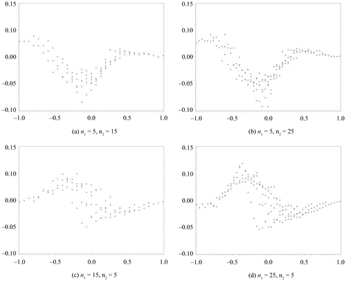
In this section, we compare the exact η defined by the MCMC method to the approximate η. We assume a non-informative prior distribution. In our computation for η via the MCMC method, we set the total number of occurrences at forty-five thousand, the burn-in term at five thousand, and the sampling interval at every ten items. We subsequently confirmed the convergence from the plot of a sample autocorrelation and the plot traced for the overall results. These results are summarized in Figures 1–4. We set the difference in sample rate (X₂/n₂−X₁/n₁) on the horizontal axis and plotted the difference between the approximate η and the exact η on the vertical axis. Figures 1 and 2 show the results obtained for the same sample size scenario (n₁ = n₂ = 10, 20, 30, 50), whereas Figures 3 and 4 show the results for the unbalanced sample size scenario (n₁, n₂) = (5, 15), (5, 25), (15, 5), (25, 5). In addition, the results depicted in Figures 1 and 3 were obtained with Δ₀ = 0.1, whereas those depicted in Figures 2 and 4 were obtained with Δ₀ = 0.2.

Figure 1. Δ₀ = 0.1.

Source: Vertical axis: The difference between approximate probability and exact probability of η. Horizontal axis: The difference between sample rate.

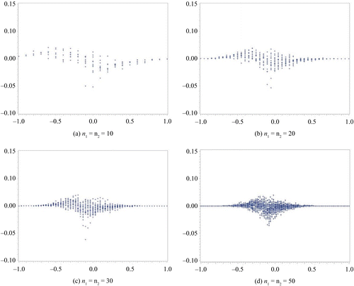
Figure 2. Δ₀ = 0.2.

Source: Vertical axis: The difference between approximate probability and exact probability of η. Horizontal axis: The difference between sample rate.

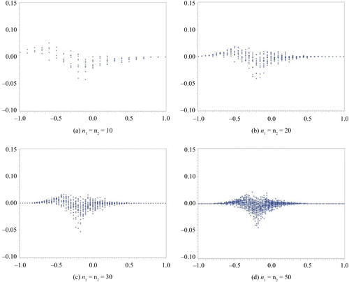
Figure 3. Δ₀ = 0.1.

Source: Vertical axis: The difference between approximate probability and exact probability of η. Horizontal axis: The difference between sample rate.

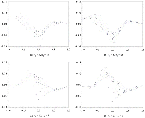
Figure 4. Δ₀ = 0.2.

Source: Vertical axis: The difference between approximate probability and exact probability of η. Horizontal axis: The difference between sample rate.

From the results depicted in Figure 1, it is clear that the difference between the approximate and exact methods is the greatest when the difference in the sample rate is approximately Δ₀. There also appears to be a tendency for η to be estimated as being higher by the exact method than the approximate method when the sample rate is negative; that is, when the proportion of X₂ is high. Conversely, the approximate method estimates a higher η than the exact method when the sample rate is positive. A difference in η between the approximate and the exact methods closer to zero within the range, which is the large difference of sample rate, is obtained by increasing the sample size.

The results depicted in Figure 2 exhibit the same tendency as those in Figure 1. The difference between the approximate method and the exact method is the greatest when the difference in the sample rate is approximately Δ₀. Although we have not included the corresponding results in this paper, this trend can also be seen when Δ₀ is set to a higher value.

From the results depicted in Figure 3, it can be seen that a larger dispersion of η appears in both the approximate and exact methods when the sample size is unbalanced than when it is equivalent. A tendency for the exact method to estimate a higher η than the approximate method can be observed when the sample rate is negative; a similar tendency is also present when the sample size is equivalent.

The results depicted in Figure 4 exhibit the same tendency as those in Figure 3. On comparing both sets of results, we discovered that the difference between the η obtained via the approximate method and that obtained via the exact method is only a gap of Δ₀; that is, an approximate difference of 0.1. Furthermore, the difference in the η calculated by each method increases when it is approximately Δ₀; that is, set as a non-inferiority parameter.

3.2. Example

In this section, we show the utility of η by applying it to the results of clinical trials. Table 1 lists the results of a double-blind, randomized study that compared the efficacy of a combination of a steroid and mizoribine (group CSM) with that of a steroid only (group S) in the treatment of patients with systemic lupus erythematosus (Tanaka et al., 2010). The primary objective of the study was to show that the relapse rate of group CSM was lower than that of group S by over 10%. The values obtained for η are listed in the rightmost column of Table 1. We adopted a non-informative prior. Consequently, both the exact η and the approximate η became similar values, indicating that the relapse rate of group CSM was lower than that of group S by over 10% with a 93.7% probability.

Table 1. Comparison of the efficacy of CSM with that of S

Group	Patient number	Exacerbation		η
		Number	AE rate	Exact	Approximate
CSM	28	11	0.39	0.936	0.937
S	29	17	0.59

Table 2 lists the results of a double-blind, randomized, phase-3 clinical trial that compared the safety of dienogest (hereafter, the study drug) and buserelin acetate (hereafter, the control drug) in the treatment of patients with endometriosis (from the assessment report of the Pharmaceuticals and Medical Devices Agency, 2007). The resulting adverse event rates, that is, one of the safety endpoints, are shown in Table 2. The primary objective of this study was to show that the occurrence rate of an adverse event for the study drug group was not inferior to that of the control drug group by more than 10%. In other words, the occurrence rate of adverse events for the study drug group was at least 10% lower than that of the control drug group. Using the non-informative prior, the approximate probability of η was obtained as 0.873 whereas the exact probability was obtained as 0.875. Therefore, the occurrence rate of the adverse events of the study drug group was not inferior to that of the control drug group by less than 10% with an 87% probability.

Table 2. Comparison of the safety of study drug with that of control drug

Drug	Patient number	Adverse effect		η
		Number	AE rate	Exact	Approximate
Study	129	454	3.52	0.875	0.873
Control	126	465	3.69

4. Discussion and conclusions

In this paper, we proposed a new index $\mathit{\eta }=P\left({\mathit{\lambda }}_{1,\text{post}}-{\mathit{\lambda }}_{2,\text{post}}<{\mathrm{\Delta }}_0|X_1,X_2\right)$ along with two computation methods: an approximate method and an exact method using the MCMC method. The approximate method is very simple to compute, whereas the exact method requires software that can utilize the MCMC method, such as SAS or WinBUGS, to perform computations. Therefore, the exact method is more complex than the approximate method. However, for small sample sizes where there are small differences in sample rate or imbalanced sample sizes in both groups, we found that the difference between the exact probability and the approximate probability only reached a maximum of 10%. Therefore, we recommend employing the exact probability for those cases.

Applying η to examples of actual clinical trials, we discovered that η is easy to understand intuitively because it delivers probability directly. Furthermore, because it uses the empirical Bayes method, we believe that this index can compute probabilities using the results of similar previously conducted clinical trials as well.

In summary, the results presented in this paper indicate that our proposed new index η is both effective and easy to understand intuitively.

Acknowledgments

The authors wish to thank the anonymous reviewers for their suggestions that helped to improve the manuscript.

Additional information

Funding

Funding. The authors received no direct funding for this research.

Notes on contributors

Yohei Kawasaki

Yohei Kawasaki received his BS degree in mathematics in 2005 and his MS and PhD degrees in mathematical science from Tokyo University of Science, Japan in 2007 and 2012, respectively. He joined the Mitsubishi Tanabe Pharma Corporation, the National Center for Global Health and Medicine, and Tokyo University of Science, in 2005, 2013, and 2014, respectively.

He has published over 80 research articles in reputed international journals. His research interests include the classical analysis, Bayesian analysis, biostatistics, and mathematical education.

He is currently a lecturer in the Department of Drug Evaluation and Informatics, School of Pharmaceutical Sciences, University of Shizuoka, Japan. He also is a guest researcher at the Shizuoka General Hospital as a Biostatistician.

References

- Graham, P. L., Mengersen, K., & Morton, A. P. (2003). Confidence limits for the ratio of two rates based on likelihood scores: Non-iterative method. Statistics in Medicine, 22, 2071–2083.10.1002/(ISSN)1097-0258
- Kawasaki, Y., & Miyaoka, E. (2012). A Bayesian inference of P(λ 1 < λ 2 ) for two Poisson parameters. Journal of Applied Statistics, 39, 2141–2152.10.1080/02664763.2012.702264
- Kawasaki, Y., & Miyaoka, E. (2013). A Bayesian non-inferiority test for two independent binomial proportions. Pharmaceutical Statistics, 12, 201–206.10.1002/pst.1571
- Kawasaki, Y., Shimokawa, A., & Miyaoka, E. (2013). Comparison of three calculation methods for a Bayesian inference of P(π1 > π2). Journal of Modern Applied Statistical Methods, 12, 256–268.
- Krishnamoorthy, K., & Thomson, J. (2004). A more powerful test for comparing two Poisson means. Journal of Statistical Planning and Inference, 119, 23–35.10.1016/S0378-3758(02)00408-1
- Li, H. Q., Tang, M. L., Poon, W. Y., & Tang, N. S. (2011). Confidence intervals for difference between two Poisson rates. Communications in Statistics-Simulation and Computation, 40, 1478–1493.10.1080/03610918.2011.575509
- Miede, C., & Mueller-Cohrs, J. (2005). Power calculation for non-inferiority trials comparing two Poisson distributions. Retrieved April 27, 2015, from http://www.lexjansen.com/phuse/2005/pk/pk01.pdf
- Ng, H. K. T., & Tang, M. L. (2005). Testing the equality of two Poisson means using the rate ratio. Statistics in Medicine, 24, 955–965.10.1002/(ISSN)1097-0258
- Patil, V. V., & Kulkarni, H. V. (2012). Comparison of confidence intervals for the Poisson mean: Some new aspect. REVSTAT—Statistical Journal, 10, 211–227.
- Pharmaceuticals and Medical Devices Agency (PMDA). (2007). Dienogest of assessment report. Tokyo: Author. (in Japanese).
- Sato, T. (1990). Confidence intervals for effect parameters common in cancer epidemiology. Environmental Health Perspectives, 87, 95–101.10.1289/ehp.908795
- Swift, M. B. (2009). Comparison of confidence intervals for a Poisson mean – further considerations. Communications in Statistics—Theory and Methods, 38, 748–759.10.1080/03610920802255856
- Tanaka, Y., Yoshikawa, N., Hattori, S., Sasaki, S., Ando, T., & Ikeda, M. (2010). Combination therapy with steroids and mizoribine in juvenile SLE: A randomized controlled trial. Pediatric Nephrology, 25, 877–882.10.1007/s00467-009-1341-4
- Rothman, K. J., & Greenland, S. (1998). Modern epidemiology. Philadelphia, PA: Lippincott Williams & Wilkins.
- Rudick, R. A., Stuart, W. H., Calabresi, P. A., Confavreux, C., Galetta, S. L., Radue, E. W., … Panzara, M. A. (2006). Natalizumab plus interferon beta-1a for relapsing multiple Sclerosis. New England Journal of Medicine, 354, 911–923.10.1056/NEJMoa044396