The effects of community interactions and quarantine on a complex network

Abstract

An adaptive complex network based on a susceptible–exposed–infectious–quarantine–recovered (SEIQR) framework is implemented to investigate the transmission dynamics of an infectious disease. The topology and its relations with network parameters are discussed. Using the primary outbreak data from the SEIQR network model, a regression model is developed to describe the relation between the quarantine rate and the key epidemiological parameters. We approximate the quarantine rate as a function of the number of individuals visiting communities and hubs, then incorporate it into the adaptive complex network to investigate the disease transmission dynamics. The proposed quantity can be estimated from the outbreak data and hence is more approachable as compared to the constant rate. Our results suggest that contact radius, hub radius, number of hubs, hub capacity and transmission rate may be important determinants to predict the disease spread and severity of outbreaks. Moreover, our results also suggest that during an outbreak, closing down certain public facilities or reducing their capacities and reducing the number of individuals visiting communities or public places, may significantly slow down the disease spread.

Keywords:

• complex network
• SEIQR model
• disease transmission
• quarantine

Public Interest Statement

It is known that diseases have a substantial impact on a social community. Understanding the spread of infectious diseases is an important key to efficiently manage them. Normally, prevention and handling of infectious diseases show the overall effects on humans and society. The proposed quarantine rate by considering the factors involved social interactions obtained from the Poisson regression equation can be used as parameter of the SEIQR network model. The results presented here may help epidemiologist and researchers to gain better insight into the transmission dynamics of infectious disease, identify key factors influencing the disease transmission, and design possible ways to reduce number of infected individuals and control the further spread of the disease.

1. Introduction

Thousands of people have died because of the spread of epidemics such as influenza, SARS, malaria and as was the case of the last Ebola epidemic in the countries of West Africa (Hethcote, Zhien, & Shengbing, 2002; Khalil, Abdel-Aziz, Nazmy, & Abdel-Badeeh Salem, 2010). The economics plays an important role in the prevention of the epidemic outbreak. For example, in the countries of West Africa, the destruction of health structures and the almost non-existent health system due to the impoverishment of the majority of the population were the main reasons for the outbreak.

Isolation and quarantine are implemented as control measures when the outbreak has reached high epidemic levels. Vaccination is one of the effective methods to control infectious diseases (especially in the endemic areas) if vaccine is available, but vaccines are not free and states have to pay a lot of money to get sufficient recourses of vaccines. In underdeveloped countries, this cost is oftentimes not affordable. Treatment is normally given to symptomatic individuals to reduce infection and hence transmission (Day, Park, Madras, Gumel, & Wu, 2006).

Quarantine is the control measure used to separate and restrict the movement of individuals who are not displaying symptoms and may have been exposed to the disease or had physical contacts with infected individuals (Agarwal & Bhadaurial, 2013; Gumel et al., 2004). It had been shown that quarantine of certain individuals is a vital strategy that can control the outbreaks due to the effective reduction of contacts between susceptible and diseased individuals (Castillo-Chavez, Carlo-Garsow, & Yakubu, 2003; Chowell, Fenimore, Castillo-Garsow, & Castillo-Chavez, 2003; Chowell et al., 2004; Gumel et al., 2004; Yan & Zou, 2008,2009).

Mathematical modelling has been as a useful tool for studying disease transmission to gain a better understanding of diseases and help design control strategies (Anderson & May, 1992; Gerberry & Milner, 2009). Bondy, Russell, Lafleche, and Rea (2009) studied the impact of community quarantine on SARS transmission in Ontario by estimating the secondary case count difference and number needed to quarantine individuals based on actual data from the 2003 Ontario, Canada, SARS outbreak. Secondary case count difference (SCCD) that reflects reduction in the average number of transmissions arising from a SARS case in quarantine, relative to not in quarantine, at onset of symptoms was estimated. They found that SCCD was approximately 0.133, estimated using Poisson and negative binomial regression models (with identity link function). The inverse of this term representing the number needed to quarantine suggested 7.5% of exposed individuals to be quarantined in community to prevent one additional case of transmission in the community. Safi and Gumel (2011) proposed a mathematical model for the transmission dynamics of an infectious disease subject to the quarantine, isolation and imperfect vaccination. Then, numerical results suggested that the singular use of a quarantine/isolation strategy could possibly lead to the effective disease control if its effectiveness level is moderately high enough. Roy (2012) proposed a mathematical model of the hand, foot and mouth disease to investigate the transmission dynamics and the effectiveness of quarantine analytically. The results showed that the disease can be controlled by quarantine of more actively infected individuals. Dobay, Gabriella Gall, Daniel Rankin, and Bagheri (2013) extended the standard SIR model by adding two quarantine categories of susceptible and infected individuals. They explored the efficiency of quarantine strategies in relation to the carrying capacity of the facility under the assumption that the quarantine rate is proportional to the amount of spare rooms inside the quarantine facility.

It is believed that human contact which is the main route of transmission of many infectious diseases can be graphically represented by complex networks (Albert & Barabasi, 2002; Newman, 2003). As the structures of networks reflects the epidemiology, the contact structures of the population and the efficacy of intervention strategies (House, Davies, Danon, & Keeling, 2009) and the contact networks have thus become a valuable tool to model the propagation of infectious diseases, and have been used widely over the last decade (Danon et al., 2011; Hai, Small, & Xin-Chu, 2009; Moore & Newman, 2000; Newman, 2002,2006; Pastor-Satorras & Vespignani, 2001; Small & Tse, 2010; Zhang & Wang, 2010). Consequently, several types of computer-generated idealized networks have been constantly proposed for studying the disease transmission. Each type of network can be distinguished from the others in the way in which the vertices are distributed on space and the vertices are connected.

The most popular types of networks used to investigate the disease transmission include random networks, lattice networks, small-world networks, spatial networks and scale-free networks. In random networks, the spatial positions of vertices are generally irrelevant, and each individual represented on the networks as a node is connected to either a fixed number of randomly chosen vertices or any of the other nodes with certain probability (Bollobás, 1985). In lattice networks, vertices are located on a regular grid of points and adjacent nodes are relatively connected. Consequently contacts between individuals on the lattice are localized in space (Keeling & Eames, 2005). Random networks generally have low clustering and short path lengths, while lattice networks have high clustering and long path lengths. Hence, it normally takes several steps to move from one node to another on the lattice networks. Small-world networks possess the characteristics of high clustering and short path lengths by adding a small number of random long-range connections to lattice networks (Keeling & Eames, 2005; Watts & Strogatz, 2002). Due to the long-range connections, in small-world networks, infection may reach all parts of the lattices relatively quickly as compared to lattice networks themselves. In spatial networks, individuals are positioned within the given area and two individuals within a given area are connected with a probability depending on their distance (Keeling & Eames, 2005; Read & Keeling, 2003). Scale-free networks have a Poisson degree distribution and can be constructed dynamically by adding new nodes to a network one by one. This mechanism can be used to imitate one of the natural features of social contacts such that a newcomer normally prefers to socialize with other individuals who are popular or equivalently have large numbers of contacts. This leads to forming of a super-spreader that plays a critical role on the disease transmission (Albert & Barabasi, 2002).

For the epidemic networks, vertices of a network represent individuals while edges describe contacts among them. The degree of a node in a network denotes the number of edges connected to the node, or simply the number of contacts of the individual. Diseases are transmitted from infected individuals to susceptible individuals from node to node. Each node is subjected to an individual’s disease status; for example, it is either susceptible to or infected by the disease. According to the disease transmission, susceptible nodes that are linked to infected nodes through edges can become infected with a certain rate. It is believed that interactions in a human society can be expressed by dynamic social networks and such networks have been useful for studying and understanding many epidemiological problems.

Previous studies have examined the quarantine and isolation strategies. Several studies have considered a constant or proportional quarantine rate (Castillo-Chavez et al., 2003; Day et al., 2006; Hethcote et al., 2002) and have not considered factors influencing the outcome of quarantine. However, some papers have considered the influence of adaptive and non-constant quarantine rates to the epidemic dynamics (e.g. Bloem, Alpcan, & Basar, 2009; Moghadas & Murray, 2006; Reppas, Tsoumanis, & Siettos 2010). In reality, the quarantine rate undoubtedly changes through time via the number of contacts as the efficacy of quarantine procedures normally increases during an outbreak and declines after. Here we take this aspect into account by examining the quarantine rate which is not constant. We examine the epidemiological parameters that can affect the outcome of quarantine by developing an SEIQR epidemic network model and determining a quarantine rate as a function obtained from statistical analysis of epidemiological data.

The SEIQR network model with regression-fit quarantine rate is developed to examine the spread of disease within populations by incorporating human contact behaviour and interactions between human and communities in this paper. In our network model, there are two types of nodes, ordinary and hub nodes, both of which are linked by dynamic links and that leads to the adaptive social network of human and societies. The rest of this work is organized as follows. Section 2 introduces our SEIQR model and its stability analysis. In Section 3, the method for constructing the adaptive social network with a constant quarantine rate is presented together with the investigation of network parameters on the disease transmission. In Section 4, Poisson regression analysis for quarantine rate is demonstrated and its effects on short and long outbreak periods of the disease are investigated. Conclusions and discussion are given in Section 5.

2. The SEIQR model and stability analysis

In this part, we modify the general SEIQR model (Gerberry & Milner, 2009) to incorporate interactions among individuals and interactions between individuals and public places. The human population (N) is categorized into five groups: susceptible (S), exposed (E), infected (I), quarantined (Q) and recovered (R). Hence, the total population size is $N(t)=S(t)+E(t)+I(t)+Q(t)+R(t)$. Next, we introduce two variables of $S_h$ and $I_h$ for public places or hubs to represent the number of uncontaminated and contaminated hubs, respectively. In this model, we make the following assumptions:

• Susceptible individuals are recruited into the population by births or migration at a constant rate A.

• Susceptible individuals enter the exposed class when they make contact with the individuals in the infectious stage at a rate $\mathit{\beta }$. The transmission is assumed to be density-dependent. Hence, the force of infection from infectious individuals is $\mathit{\beta }I$.

• The infected hubs can spread the disease to some visiting susceptible people at rate ${\mathit{\beta }}^{\prime }$. The force of infection from infected hubs is defined by ${\mathit{\beta }}^{\prime }\mathit{\delta }(I_h)I_h$ where $\mathit{\delta }(I_h)$ is defined by: (1) $$\begin{array}{c}\hfill \mathit{\delta }(I_h)=\left\{\begin{array}{cc}1\hfill & \text{if}S\text{visits}{I}_h,\hfill \\ 0\hfill & \text{otherwise}.\hfill \end{array}\right.\end{array}$$(1)

• Exposed individuals become infectious after an incubation period $1/\mathit{\alpha }$.

• Infected individuals either recover naturally at a rate $\mathit{\gamma }$ or are immediately removed to the quarantine class at a rate $\mathit{\eta }$.

• Quarantined individuals remain in the quarantine class until they are no longer infectious and acquire immunity. Hence, it is assumed that they enter the recovered class at a rate $\mathit{\epsilon }$.

• The natural death rate of individuals is $\mathit{\mu }$.

• We make an additional assumption that individuals who are exposed to the disease can become immune to the disease (Tiantian & Yakui, 2013) at a rate $\mathit{\kappa }$.

• A susceptible hub becomes an infected hub if at least one infected individual visits the hub. The force of infection from infectious people on the susceptible hub is defined by $\mathit{\delta }(S_h)I$ where $\mathit{\delta }(S_h)$ is defined by: (2) $$\begin{array}{c}\hfill \mathit{\delta }(S_h)=\left\{\begin{array}{c}1\text{if}I\text{visits}{S}_h,\hfill \\ 0\text{otherwise}.\hfill \end{array}\right.\end{array}$$(2)

• An infected hub will recover and will rejoin the susceptible class if no infected individual has visited such infected hub for infectious period. The force of recovery from susceptible hub on the infected hub is given by ${\mathit{\gamma }}_h{I}_h$.

The size population of each individual group varies with time according to the following SEIQR model:(3) $$\begin{array}{cc}\hfill \dot{S}& =A-[\mathit{\beta }SI+{\mathit{\beta }}^{\prime }\mathit{\delta }(I_h)S{I}_h]-\mathit{\mu }S,\hfill \\ \hfill \dot{E}& =[\mathit{\beta }SI+{\mathit{\beta }}^{\prime }\mathit{\delta }(I_h)S{I}_h]-(\mathit{\mu }+\mathit{\alpha }+\mathit{\kappa })E,\hfill \\ \hfill \dot{I}& =\mathit{\alpha }E-(\mathit{\mu }+\mathit{\eta }+\mathit{\gamma })I,\hfill \\ \hfill \dot{Q}& =\mathit{\eta }I-(\mathit{\mu }+\mathit{\epsilon })Q,\hfill \\ \hfill \dot{R}& =\mathit{\kappa }E+\mathit{\gamma }I+\mathit{\epsilon }Q-\mathit{\mu }R,\hfill \end{array}$$(3)

whereas the disease dynamics of public places (or hub nodes) can be described by(4) $$\begin{array}{cc}\hfill \dot{S_h}& =-{\mathit{\beta }}_h\mathit{\delta }(S_h)I{S}_h+{\mathit{\gamma }}_h{I}_h,\hfill \\ \hfill \dot{I_h}& ={\mathit{\beta }}_h\mathit{\delta }(S_h)I{S}_h-{\mathit{\gamma }}_h{I}_h.\hfill \end{array}$$(4)

From Equations (3) and (4),(5) $$\begin{array}{c}\hfill \frac{\text{d}{N}_p}{\text{dt}}=\frac{\text{d}(S+E+I+Q+R)}{\text{dt}}=A-\mathit{\mu }N,\frac{\text{d}{N}_h}{\text{dt}}=\frac{\text{d}(S_h+I_h)}{\text{dt}}=0,\end{array}$$(5)

where $N=N_p+N_h$.

In this work, we assume that the total population and the number of public places are fixed. Hence,(6) $$\begin{array}{c}\hfill A=\mathit{\mu }N,\end{array}$$(6)

where N and $N_h$ are constants.

Consequently, the disease-free steady state is given by(7) $$\begin{array}{c}\hfill P^0=(S,E,I,Q,R,S_h,I_h)=(N,0,0,0,0,N_h,0)\end{array}$$(7)

and the disease-present steady state is as follows:(8) $$\begin{array}{c}\hfill P^{\ast }=(S^{\ast },E^{\ast },I^{\ast },Q^{\ast },R^{\ast },S_h^{\ast },I_h^{\ast })\end{array}$$(8)

where(9) $$\begin{array}{cc}\hfill S^{\ast }& =\frac{(\mathit{\mu }+\mathit{\alpha }+\mathit{\kappa })(\mathit{\mu }+\mathit{\eta }+\mathit{\gamma })}{\mathit{\alpha }(\mathit{\beta }+{\mathit{\beta }}^{\prime })},\hfill \\ \hfill E^{\ast }& =\frac{D^{\prime }\mathit{\delta }(I_h)I_h^{\ast }}{\mathit{\alpha }},\hfill \\ \hfill I^{\ast }& =\mathit{\delta }(I_h)I_h^{\ast },\hfill \\ \hfill Q^{\ast }& =\frac{\mathit{\eta }\mathit{\delta }(I_h)I_h^{\ast }}{\mathit{\mu }+\mathit{\epsilon }},\hfill \\ \hfill R^{\ast }& =\frac{\mathit{\delta }(I_h)I_h^{\ast }(\mathit{\kappa }{D}^{\prime }+\mathit{\gamma }+\mathit{\epsilon }\mathit{\eta })}{\mathit{\mu }\mathit{\alpha }{D}^{″}},\hfill \\ \hfill S_h^{\ast }& =\frac{{\mathit{\gamma }}_h}{{\mathit{\beta }}_h\mathit{\delta }(S_h)\mathit{\delta }(I_h)},\hfill \\ \hfill I_h^{\ast }& =N_h-S_h,\hfill \end{array}$$(9)

where $D^{\prime }=\mathit{\gamma }+\mathit{\eta }+\mathit{\mu }$ and $D^{″}=\mathit{\epsilon }+\mathit{\mu }$.

Let ${\tilde{\mathbf{F}}}_i(x)$ be the rate of appearance of new infections in the compartment i, ${\tilde{\mathbf{V}}}_i^{+}(x)$ be the rate of transfer of individuals into the compartment i by all other means, and ${\tilde{\mathbf{V}}}_i^{-}(x)$ be the rate of transfer of individuals out of the compartment i. According to van den Driessche and Watmough (2002), ${\dot{x}}_i={\tilde{\mathbf{F}}}_i(x)-{\tilde{\mathbf{V}}}_i(x)$ where ${\tilde{\mathbf{V}}}_i(x)={\tilde{\mathbf{V}}}_i^{-}(x)-{\tilde{\mathbf{V}}}_i^{+}(x)$. Hence,$$\tilde{\mathbf{F}}=\left[\begin{array}{c}\mathit{\beta }SI+{\mathit{\beta }}^{\prime }\mathit{\delta }(I_h)S{I}_h\hfill \\ 0\hfill \\ \mathit{\delta }(S_h)I{S}_h\hfill \\ 0\hfill \\ 0\hfill \\ 0\hfill \\ 0\hfill \end{array}\right]\text{and}\tilde{\mathbf{V}}=\left[\begin{array}{c}(\mathit{\mu }+\mathit{\alpha }+\mathit{\kappa })E\hfill \\ (\mathit{\mu }+\mathit{\eta }+\mathit{\gamma })I-\mathit{\alpha }E\hfill \\ {\mathit{\gamma }}_h{I}_h\hfill \\ (\mathit{\mu }+\mathit{ϵ})Q-\mathit{\eta }I\hfill \\ \mathit{\beta }SI+{\mathit{\beta }}^{\prime }\mathit{\delta }(I_h)S{I}_h+\mathit{\mu }S-A\hfill \\ \mathit{\delta }(S_h)I{S}_h-{\mathit{\gamma }}_h{I}_h\hfill \\ \mathit{\mu }R-\mathit{\kappa }E-\mathit{\gamma }I-\mathit{ϵ}Q\hfill \end{array}\right].$$

Next, we introduce a vector $\mathit{X}$ with new arrangements of disease classes:(10) $$\begin{array}{c}\hfill \mathit{X}={[E,I,I_h,Q,S,S_h,R]}^{\text{T}}\end{array}$$(10)

The infected population includes individuals from E, I, $I_h$ and Q classes in our case. The disease-free equilibrium arranged according to X is described by(11) $$\begin{array}{c}\hfill {\mathit{X}}_0={[0,0,0,0,N,N_h,0]}^{\text{T}}\end{array}$$(11)

Let $\widehat{\mathbf{F}}$ be the $m\times m$ matrix of infected individuals through various diseased compartments which is defined by $\widehat{\mathbf{F}}=\left[\frac{\mathit{\partial }{\mathbf{F}}_i}{\mathit{\partial }{\mathit{X}}_j}({\mathit{X}}_0)\right]$ and $\widehat{\mathbf{V}}=\left[\frac{\mathit{\partial }{\mathbf{V}}_i}{\mathit{\partial }{\mathit{X}}_j}({\mathit{X}}_0)\right]$, $i,j=1,2,3,4$. Hence,$$\begin{array}{c}\hfill \widehat{\mathbf{F}}(\mathbf{X})=\left[\begin{array}{cccc}0& \mathit{\beta }S& {\mathit{\beta }}^{\prime }\mathit{\delta }(I_h)S& 0\\ 0& 0& 0& 0\\ 0& \mathit{\delta }(S_h)S_h& 0& 0\\ 0& 0& 0& 0\end{array}\right]\end{array}$$

and$$\begin{array}{c}\hfill \widehat{\mathbf{V}}(\mathbf{X})=\left[\begin{array}{cccc}\mathit{\mu }+\mathit{\alpha }+\mathit{\kappa }& 0& 0& 0\\ -\mathit{\alpha }& \mathit{\mu }+\mathit{\eta }+\mathit{\gamma }& 0& 0\\ 0& 0& {\mathit{\gamma }}_h& 0\\ 0& -\mathit{\eta }& 0& \mathit{\mu }+\mathit{ϵ}.\end{array}\right].\end{array}$$

We define $\mathbf{F}$ and $\mathbf{V}$ as the matrices at ${\mathit{X}}_0$ obtained from $\mathbf{F}$ and $\mathbf{V}$, respectively. Thus,$$\begin{array}{c}\hfill \mathbf{F}=\left[\begin{array}{cccc}0& \mathit{\beta }N& {\mathit{\beta }}^{\prime }\mathit{\delta }(I_h)N& 0\\ 0& 0& 0& 0\\ 0& \mathit{\delta }(S_h)N_h& 0& 0\\ 0& 0& 0& 0\end{array}\right]\end{array}$$

and$$\begin{array}{c}\hfill \mathbf{V}=\left[\begin{array}{cccc}\mathit{\mu }+\mathit{\alpha }+\mathit{\kappa }& 0& 0& 0\\ -\mathit{\alpha }& \mathit{\mu }+\mathit{\eta }+\mathit{\gamma }& 0& 0\\ 0& 0& {\mathit{\gamma }}_h& 0\\ 0& -\mathit{\eta }& 0& \mathit{\mu }+\mathit{ϵ}\end{array}\right].\end{array}$$

Hence,$$\begin{array}{c}\hfill {\mathbf{F}V}^{-1}=\left[\begin{array}{cccc}\frac{\mathit{\beta }\mathit{\alpha }N}{(\mathit{\mu }+\mathit{\alpha }+\mathit{\kappa })(\mathit{\eta }+\mathit{\gamma })}& \frac{\mathit{\beta }N}{\mathit{\mu }+\mathit{\eta }+\mathit{\gamma }}& \frac{{\mathit{\beta }}^{\prime }\mathit{\delta }(I_h)N}{{\mathit{\gamma }}_h}& 0\\ 0& 0& 0& 0\\ \frac{\mathit{\alpha }\mathit{\delta }(S_h)N_h}{(\mathit{\mu }+\mathit{\alpha }+\mathit{\kappa })(\mathit{\eta }+\mathit{\gamma })}& \frac{\mathit{\delta }(S_h)N_h}{\mathit{\mu }+\mathit{\eta }+\mathit{\gamma }}& 0& 0\\ 0& 0& 0& 0\end{array}\right].\end{array}$$

The reproductive number $R_0$ following Diekmann, Heesterbeek, and Metz (1990) and van den Driessche and Watmough (2002) can be calculated from the formula: $R_0=\mathit{\rho }({\mathbf{F}V}^{-1})$ where $\mathit{\rho }({\mathbf{F}V}^{-1})$ is the spectral radius of ${\mathbf{F}V}^{-1}$ and ${\mathbf{F}V}^{-1}$ is called the next generation matrix for the model. We then obtain$$\begin{array}{c}\hfill R_0=\frac{1}{2}\frac{\mathit{\beta }\mathit{\alpha }{\mathit{\gamma }}_{h}N+\sqrt{{\mathit{\beta }}^2{N}^2{\mathit{\alpha }}^2{\mathit{\gamma }}_h^2+4\mathit{\alpha }\mathit{\delta }(S_h)N_h{\mathit{\beta }}^{\prime }\mathit{\delta }(I_h)N{\mathit{\gamma }}_h(\mathit{\mu }+\mathit{\alpha }+\mathit{\kappa })(\mathit{\eta }+\mathit{\gamma })}}{{\mathit{\gamma }}_h(\mathit{\mu }+\mathit{\alpha }+\mathit{\kappa })(\mathit{\eta }+\mathit{\gamma })}\end{array}$$

If $R_0<1$, ${\mathit{X}}_0$ is locally asymptotically stable or the disease dies out, and if $R_0>1$, ${\mathit{X}}_0$ is unstable or the disease is present.

3. The SEIQR network model with a constant quarantine rate

To investigate the disease transmission that mimics social human activities by taking into account interactions between humans and humans and between humans and communities, we propose an adaptive social network model based on the SEIQR framework. The network consists of $N_p$ ordinary nodes (people) and $N_h$ dynamic hub nodes (public places) with connecting links within a unit square region. On the network, ordinary nodes represent individuals or groups of individuals, while hub nodes represent public facilities such as schools, hospitals and shopping centres. The nodes are located in the unit square randomly with the constraints that the distance between any two hub nodes (ordinary nodes) is greater than $d_{hmin}$ ($d_{min}$) and the distance between a hub node and any ordinary node is greater than $d_{homin}$. The use of the minimum distances between different nodes is to ensure that the nodes do not get too close.

To describe the neighbourhood contact between individuals (ordinary nodes), each ordinary node is connected to its surrounding nodes provided that the distance between them is less than its contact radius $R_c$. Let $N_i$ be the set of neighbouring nodes of the node i with connections to i, then we have $N_i=\{j|d_{ij}<R_c\}$ where $d_{ij}$ is the distance between nodes i and j. As the hub nodes are used to represent public facilities, they may be visited by different nodes (individuals) at different time up to certain amount. To describe this nature, the links from individuals to the hubs should be dynamic and each hub node is equipped with two parameters, contact radius $R_h$ and the hub node capacity $C_h$. The hub node contact radius is used to define the contact region, ${\mathit{\omega }}_h=\{(x,y)|{(x-x_h)}^2+{(y-y_h)}^2<R_h^2\}$ where $(x_h,y_h)$ is the coordinate of the hub node, within which every node may be connected to the hub; while the hub node capacity refers to the number of links between the hub node and the ordinary nodes within the contact region. The links between the hub node and ordinary nodes vary with time randomly to reflect the dynamic feature of social networks. Obviously, If $R_c=\sqrt{2}$, it is a homogenous uniform mixing network in which every node has $N-1$ edges (degree) and each node connects to all the other $N-1$ nodes. Otherwise, it is a heterogeneous network in which the degree of each node is the number of its neighbours with connection to it. For the network with hubs, $N_h>0$, we have an adaptive network. A numerical algorithm has been developed to construct the dynamic network and examine its various properties.

The SEIQR ordinary differential equation model as mentioned in Section 2 is based on the assumption that the population is fully mixed, namely the infected individuals have equal chance to contact other individuals and that all contacts transmit the disease with the same probability. Obviously, these assumptions are oversimplified in real life. However, the network model can remove these assumptions as the infected individuals transmit the disease with a certain probability to those who only link to it. In our simulation, there are 1,000 nodes including nine hub nodes and the others are people nodes. Moreover, people nodes are categorized into 20 communities and randomly located in a unit square. A single node belongs to one community and it is allowed to visit any one hub per time. Any people nodes in a contact radius $R_c$ of each node are neighbours of such node. In meanwhile, any node in a hub radius has opportunity to visit hub at an instant time. The numbers of edges linked to each hub then varies according to time.

As the network parameters play an important role in describing the topology of the network, we investigate the impact of them on the network and the disease spread according to: (1) properties of ordinary nodes by focusing on a contact radius: (2) properties of hub nodes including hub contact radius ($R_h$), number of hubs ($N_h$), hub capacity ($C_h$), and (3) properties of a disease by focusing on a transmission rate.

3.1. Network analysis on a contact radius

Firstly, we investigate the influence of neighbourhood contact radius, $R_c$, the topology of the network. Figure 1 shows three different topologies for part of the network corresponding to three different contact radius values, 0.05, 0.07 and 0.09. The network with a higher contact radius leads to more contacts with other nodes. Figure 2 shows the effects of varying the contact radius on the average degree. It can be clearly seen in Figure 2 that, as the contact radius increases, the average degree increases. The effect of contact radius on the degree distribution of the proposed network is also investigated for various values of the contact radius. Figure 3 shows a plot of degree distribution for various contact radius $R_c$ values. The peak value of degree distribution of network with smaller contact radius is higher than network with larger contact radius. It indicates that the average degree of a network is higher for a larger contact radius.

Figure 1. Topology of a network with no hub ($N_h=0$) for three different values of the neighbourhood contact radii $R_c$: (a) $R_c=0.05$; (b) $R_c=0.07$; (c) $R_c=0.09$.Note: Blue—susceptible, Green—exposed, Red—infected, Violet—quarantine, and Yellow—recovered.

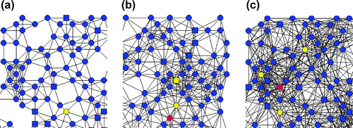
Figure 2. Dependence of the average degree according to the contact radius.

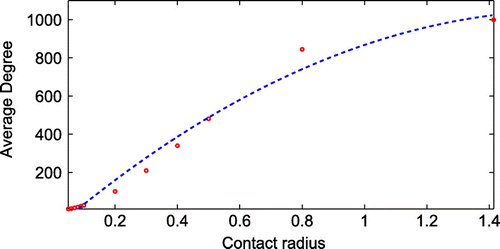
Figure 3. Degree distribution of the heterogeneous network with various nodal contact radii $R_c$ of 0.05, 0.06, 0.07, 0.08 and 0.09 (from the left to the right curves).

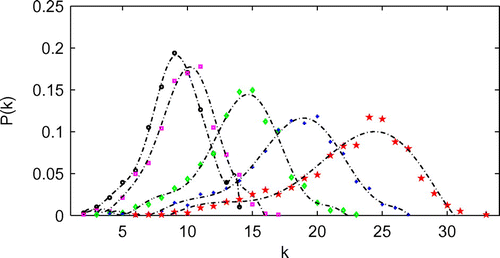
Figure 4. Simulation results from the SEIQR network model with transmission probabilities $\mathit{\beta }$ of 0.004 and three different contact radii: (a) $R_c=0.035$; (b) $R_c=0.055$; (c) $R_c=0.075$.

As human contact is an important mechanism of the disease transmission, we investigate the influence of contact radius on the disease transmission. For $d_{min}<R_c<\sqrt{2}$, the influence of $R_c$ on the transmission of diseases is shown in Figure 4. As the contact radius decreases, the peak value of infected population decreases significantly and the time when the peak value occurring prolongs. The length of contact radius affects the severity through the number of infected people and the epidemic time.

3.2. Network analysis on properties of hub nodes

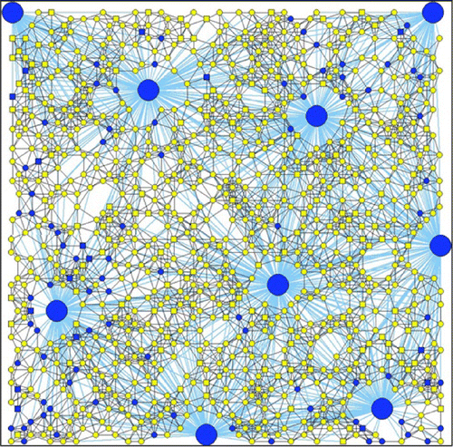
Since transmission between contaminated public places and individuals is taken into account in the model apart from transmission between individuals, we can additionally investigate the influence of hub parameters on the disease transmission. In addition, as hubs are used to represent public facilities, and the number of hubs and hub parameters can be controlled in the control of disease transmission, it may be useful to gain a better insight into how they influence the transmission dynamics of the disease. Figure 5 shows the network topology with nine hubs used for numerical analysis.

Figure 5. The adaptive network including both people and hub nodes used in this study.Note: Blue—susceptible, Green—exposed, Red—infected, Violet—quarantine, and Yellow—recovered.

The number of hubs and the hub node parameters also has significant influences on the network properties. Figure 6 shows the network structures at three different times (t = 15, 20 and 25 days) for the adaptive network with contact radius $R_c$ of 0.06, hub radius $R_h$ of 0.30 and hub capacity $C_h$ of 15 visitors per day. Disease statuses of individuals and the links between individuals, communities and public places change over time. At 15 days after a few infected individuals are introduced, all nodes are still susceptible, while at 20 days there are some nodes becoming exposed or infected. At 25 days, some of the nodes which are exposed or infected recover. It is also noted that a change of the visiting probability per day leads to change in the node-hub links of the network.

Figure 7 demonstrates the effect of numbers of hubs on the degree distribution of the network model with contact radius $R_c$ of 0.06 and hub radius $R_h$ of 0.25. It is shown that the degree distribution of the network model with different numbers of hubs has a similar pattern. Tables 1 and 2 show the effects of the number of hubs and hub contact radius on the average degree (nodal contact number). The results suggest that as the number of hubs and hub contact radius increase, the average degree increases.

Figure 6. A particular part of the topology of a nine-hub adaptive network with contact radius $R_c$ of 0.06 and hub radius $R_h$ of 0.30 at three different times: (a) t = 15 days; (b) t = 20 days; (c) t = 25 days. Note: Blue—susceptible, Green—exposed, Red—infected, Violet—quarantine, and Yellow—recovered.

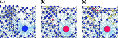
Figure 7. Effects of the number of hubs on degree distribution of the network model with $R_c=0.06$ and $R_h=0.30$.

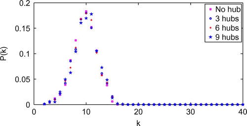
Table 1. Average degree for different number of hubs having $R_c$ = 0.06 with $R_h$ = 0.4

Number of hubs	Average degree
0	9.6797
3	9.7739
6	9.7939
9	9.8636
12	9.9434

Table 2. Average degree of node in the network model with nodal contact radius 0.6 and nine hubs having different hub-contact radii

Hub radius	Average degree
0.25	9.60
0.35	9.82
0.45	9.86
0.55	9.95

Figure 8. Simulation results from the SEIQR network model with nodal contact radius of 0.06 and various numbers of hubs having the contact radius of 0.30: (a) $N_h=5$; (b) $N_h=7$; (c) $N_h=9$.

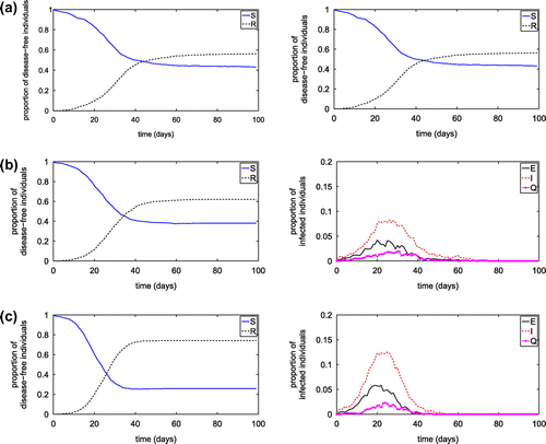
Figure 9. Simulation results from the SEIQR network model with three different hub capacities: (a) $C_h=25\%$; (b) $C_h=50\%$; (c) $C_h=75\%$.

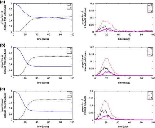
Figure 10. Simulation results from the SEIQR network model with nodal contact radius $R_c$ of 0.055 and nine hubs having three different hub contact radii: (a) $R_h=0.20$; (b) $R_h=0.30$; (c) $R_h=0.40$.

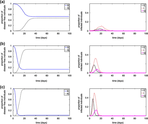
Figure 11. Effect of transmission probability $\mathit{\beta }$ on the disease spread in the network model with ${\mathit{\beta }}^{\prime }=0.04$, $R_c=0.055$, $R_h=0.40$: (a) $\mathit{\beta }=0:03$; (b) $\mathit{\beta }=0:06$; (c) $\mathit{\beta }=0:09.$

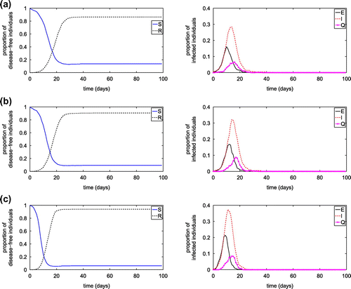
Figure 12. Effect of transmission probability $\mathit{\beta }$ on the proportion of infected individual at the steady state.

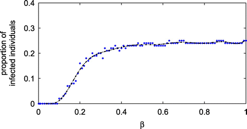
Figure 8 shows the influence of the number of hubs, while Figures 9 and 10 show the influences of hub capacity and hub contact radius on the transmission of diseases on the SEIQR network with transmission probabilities $\mathit{\beta }$ of 0.004 and ${\mathit{\beta }}^{\prime }$ of 0.004 from an infected node to a susceptible node, and from infected hub to a visiting susceptible node, respectively. The reduced hub number, hub capacities and/or hub contact radius may significantly influence the disease transmission, including reducing the peak value of infected population and prolong the occurring of the peak value.

3.3. Network analysis on properties of a disease by focusing on a transmission rate

There are many factors affecting the spread pattern of infectious diseases. Among those factors, transmission rate plays an essential role for the disease transmission. Herein, effects of the transmission probability $\mathit{\beta }$ are explored. Figure 11 shows the effect of the transmission probability of the disease spread on the network for the visiting probability of 0.05. The results show a faster spread of the disease and the higher number of infected individual for a higher transmission probability following that individuals with a higher transmission rate have more chance to catch the disease. To investigate the effect of transmission rate, we vary the value of $\mathit{\beta }$ from 0 to 1, while keeping other parameters the same as in Table 3. The results, given in Figure 12, show that the proportion of infected individuals increases dramatically for $\mathit{\beta }$ between 0.1 and 0.4.

4. The SEIQR network model with a regression-fit quarantine rate

In this section, we investigate the quarantine rate as a function of the network parameters, in comparison to the constant quarantine rate. The formula for the quarantine rate is developed by the statistical method.

Starting from an initial state, nearly all nodes are set to be susceptible and for a few nodes are set to be infectious. The disease status of each individual node evolves in time depending on its previous state and the connections with other individuals in different disease statuses. Five dynamic processes occur on the network. The first dynamic process is the transmission of disease from infected to susceptible individuals leading to the change of status of some susceptible individuals to exposed individuals (S to E). Then the probability for each of these nodes to change its status from S to E is $\mathit{\beta }$, and a random process is used to determine the status of these nodes. The second dynamic process is the change of status of the exposed individuals to infected nodes, which is done after being exposed $1/\mathit{\alpha }$ time steps. The third dynamic process is the change of infected individuals from status I to Q after being infected for $1/\mathit{\eta }$ time steps. The fourth dynamic process is the change of quarantined and infected individuals (Q or I) to the recovered status (R) following the infectious period of $1/\mathit{\epsilon }$ and $1/\mathit{\gamma }$ time steps, respectively. Lastly, the fifth dynamic process is the change of exposed individuals (E) to the recovered status (R) after being exposed $1/\mathit{\kappa }$ time steps.

Table 3. Parameter values used in numerical simulation of the SEIQR epidemic network model

Biological description	Parameters	Values
Neighbourhood contact radius	$R_c$	0.055
Hub radius	$R_h$	0.4
Number of hubs	$N_h$	9
Transmission rate of infected node	$\mathit{\beta }$	0.004
Transmission rate of infectious hub	${\mathit{\beta }}^{\prime }$	0.004
Transfer rate from E to I	$\mathit{\alpha }$	1/4
Transfer rate from I to R	$\mathit{\gamma }$	1/6
Quarantine rate of infectious	$\mathit{\eta }$	0.1
Transfer rate from E to R	$\mathit{\kappa }$	0.01
Recover rate from Q to R	$\mathit{\epsilon }$	0.1
The death rate	$\mathit{\mu }$	0.01
The transmission rate from infected individual to susceptible hub	${\mathit{\beta }}_h$	1
The transfer rate at which infectious hub becomes susceptible hub	${\mathit{\gamma }}_h$	1

Throughout the numerical study, it is assumed that $S(0)=987$, $E(0)=0$, $I(0)=4$, $Q(0)=0$ and $R(0)=0$. Parameters used in the network model are described in Table 3.

One of the most important aims for studying disease transmission is to find the possible ways to limit the disease outbreak through control strategies such as isolation, quarantine and vaccination. In real practice, the quarantine rate is often unknown. In this study, we aim to propose the formula for this important quantity based on the available network data and statistical methods.

4.1. Poisson regression analysis for quarantine rate

Poisson regression is widely used to model count data: for instance, insurance data, health care data (Ismail & Zamani, 2013). In our analysis, we use the primary data obtained from the SEIQR network model with a constant quarantine rate to investigate the association of the number of quarantined individuals per time, the number of individuals visiting communities, and the number of individuals visiting hub or public places. In statistical analysis, the outcome is the number of quarantined individuals (nq) which is a count variable. The predictor variables of interest are the number of individuals visiting communities (nc) and the number of individuals visiting public places (nh). As our observations are non-negative integers and not over-dispersed, negative binomial and zero-inflated Poisson regression models may not be suitable. For this work, the quarantine rate is estimated using Poisson regression with log link function.

Figure 13. Snapshot of specification of the Poisson regression model obtained from R program.

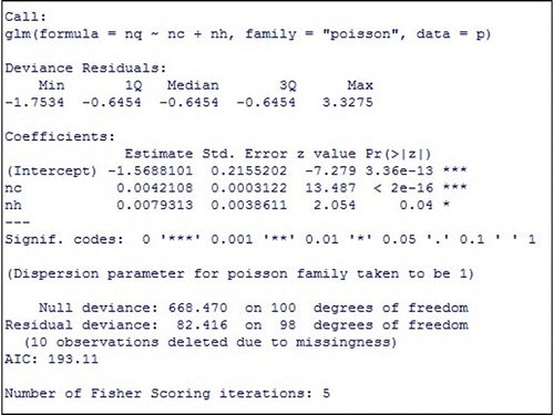
In Figure 13, apart from the regression coefficients, we obtain the standard error, z-value, and p-values. If the statistical significance of a coefficient displayed by p-value is less than 0.05, it indicates that the predictor variables related to the coefficient has statistically significant effect on the outcome variable or the number of quarantined individuals.

The result suggests that the number of individuals visiting communities and the number of individuals visiting public places per time during the outbreak are the significant predictors of the number of quarantined individuals during the outbreak.

Figure 14. Output of comparing the deviance.

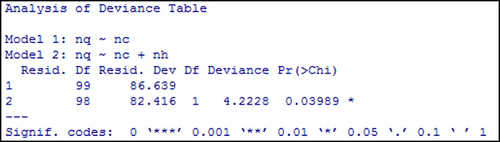
We also investigate the overall impact of the number of individuals visiting public places (nh) by comparing the deviance of full model with the deviance of model excluding (nh). The output in Figure 14 expresses that the number of individuals visiting public places (nh) is a statistical predictor of the number of quarantined individuals (nq) and all predictor variables are significant when they were taken into the model as shown in Figure 15.

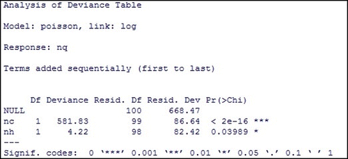
Figure 15. Goodness-of-fit test of Poisson regression model.

Consequently, we determined the estimated regression equation as follows:(12) $$\begin{array}{c}\hfill log(\text{nq})=-1.5688161+0.0042108\text{nc}-0.0079313\text{nh}.\end{array}$$(12)

The above equation implies that (nq) is the exponential function of predictor variables (nc and nh):(13) $$\begin{array}{c}\hfill \text{nq}=exp(-1.5688161+0.0042108\text{nc}-0.0079313\text{nh}).\end{array}$$(13)

Hence, the quarantined rate can be sufficiently estimated by (nq) in Equation (13) obtained from the Poisson regression model with the log link function.

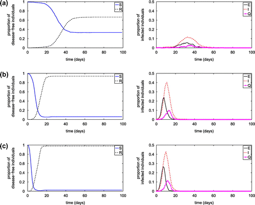
Figure 16. Simulation results of SEIQR network model with different quarantine rate. (a) Proportion of susceptible individuals; (b) Proportion of exposed individuals; (c) Proportion of infected individuals; and (d) Proportion of quarantined individuals.

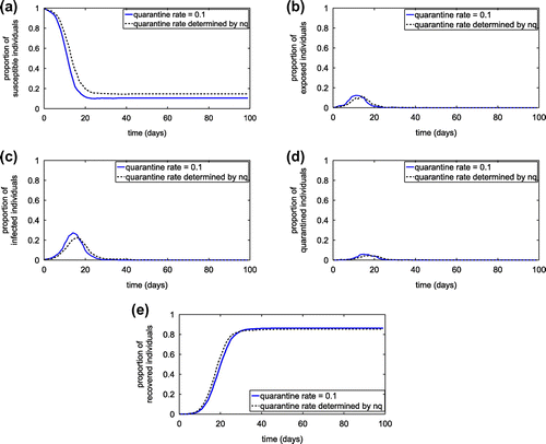
After obtaining the estimated quarantined rate as a function of the number of individuals visiting communities per time (nc), and the number of individuals visiting public places per time (nh), it is incorporated into the complex network model to investigate the transmission dynamics of the infection disease. Figure 16 demonstrates the proportion of individuals in each diseases status in comparison to the result obtained from the network model with the constant quarantine rate. The results imply that our proposed formula for the quarantine rate can be reasonably used to approximate the constant quarantine rate which may be difficult to acquire in real practice. Moreover, the formula also suggests that the number of individuals visiting communities and the number of individuals visiting public places may have the impact on the quarantine rate and consequently play a crucial role in designing a quarantine strategy.

5. Conclusions and discussion

It is believed that network models have an important role in providing a wealth of tools in gaining a better understanding into epidemiology of infectious diseases, predicting outcomes of the outbreaks and helping to design control strategies (Danon et al., 2011; Keeling & Eames, 2005). An adaptive social network based on the SEIQR model with regression-fit quarantine rate is proposed to investigate the transmission dynamics of a directly transmitted disease such as SARS or influenza. The proposed network is equipped with dynamic links between individuals, communities and public places to reflect realistic interactions in the human society. As a network can be characterized by a set of parameters such as a contact radius, the number of hub nodes and the hub node capacity, it may be important to understand how such parameters influence the transmission dynamics of a disease on the network. It is found that the hub capacity and the number of hubs among individuals affect the number of infected cases in the population. The higher the hub capacity, the higher the number of infected individuals. Our results also suggest that closing down certain hubs or reducing the capacity of certain hubs is one of the efficient ways to control the spread of an infectious disease. Moreover, we found that the larger contact radius leads to the higher number of infected individuals and the more severe outbreak. This result suggests that more isolated societies may have fewer infected cases and less severity of outbreak.

Quarantine is one of the effective means to control the spread of infectious diseases and is often implemented at the beginning of an outbreak. In general, it can be difficult to determine an appropriate quarantine rate proficiently or eliminate the disease. Hence, in this study, we investigate factors that influence the quarantine rate and approximate the quarantine rate as a function of such factors that are more attainable and easy to be quantified. To obtain the quarantine rate as a function of the number of individuals visiting communities and public places, we employ a Poisson regression model and conduct a statistical analysis. After incorporating the regression function of the quarantine rate into the network model, the proposed quarantine rate can fairly capture the transmission of the disease. However, as our rate is the function of two variables that can be relatively obtained from the data, the proposed function may be used to determine and may be a better representation of the quarantine rate. Generally, as people tend to go to communities or public places less often when they are infected, using our proposed rate may be able to capture this important feature of human behaviour while a constant one could not.

Last but not least, our findings also suggest that as it may not be feasible to quarantine a large population of individuals, promoting a strategy to decrease the number of individuals visiting communities and public places may be one of the effective ways to limit the quarantined cases and reduce resource usage.

Additional information

Funding

This research is supported by Sisaket Rajabhat University and partially supported by Prof. Dr Tab Nilaniti Foundation Scholarship and Mahidol University.

Notes on contributors

Benjamas Chimmalee

Benjamas Chimmalee is currently a PhD student at Mahidol University, Bangkok, Thailand. Her research interests are mathematical model, network model for studying disease transmission and statistical modelling in epidemiology.

Wannika Sawangtong

Wannika Sawangtong received a PhD in Mathematics from Mahidol University, Bangkok, Thailand. Currently, she is a lecturer at Mahidol University, Bangkok, Thailand. She is a vigorous researcher in the area of mathematical modelling in disease transmission and complex network of disease transmission. She has research papers published in reputed national and international journals, including Scopus.

Benchawan Wiwatanapataphee

Benchawan Wiwatanapataphee is an associate professor in the Department of Mathematics and Statistics, Curtin University, Perth, Australia. She received her PhD in Applied Mathematics from Curtin University, Perth, Australia. She is actively involved in the field of mathematical models and her specialty areas are network models, fluid flow and heat transfer models, and software development using C++. She has published more than 140 researches publications in reputed international journals.

References

- Agarwal, M., & Bhadauria, A. S. (2013). Effect of quarantine in epidemic model with saturating contact rate. Journal of Applied Mathematics and Mechanics, 9, 90–105.
- Albert, R., & Barabasi, A.-L. (2002). Statistical mechanics of complex networks. Review of Modern Physics, 74, 47–97.
- Anderson, R. M., & May, R. M. (1992). Infectious diseases of humans. Oxford: Oxford University Press.
- Bollob\’{a}s, B. (1985). Random graphs (London Mathematical Society Monograph). London: Academic Press.
- Bloem, M., Alpcan, T., & Basar, T. (2009). Optimal and robust epidemic response for multiple networks. Control Engineering Practice, 17, 525–533.
- Bondy, S. J., Russell, M. L., Lafleche, J. M. L., & Rea, E. (2009). Quantifying the impact of community quarantine on SARS transmission in Ontario: Estimation of secondary case count difference and number needed to quarantine. BMC Public Health, 9, 488.
- Castillo-Chavez, C., Carlo-Garsow, W., & Yakubu, A. A. (2003). Mathematical models of isolation and quarantine. The Journal of the American Medical Association, 290, 2876–2877.
- Chowell, G., Castillo-Chavez, C., Fenimore, P. W., Kribs-Zaleta, C. M., Arriola, L., & Hyman, J. M. (2004). Model parameters and outbreak control for SARS. Emerging Infectious Disese, 10, 1258–1263.
- Chowell, G., Fenimore, P. W., Castillo-Garsow, C., & Castillo-Chavez, M. A. (2003). SARS outbreaks in Ontario, Hong Kong and Singapore: The role diagnosis and isolation as a control mechanism. Journal of Theoretical Biology, 224, 1–8.
- Danon, L., Ford, A. P., House, T., Jewell, C. P., Keeling, M. J., Roberts, G. O., ... Vernon, M. C. (2011). Network and the epidemiology of infectious disease. Interdisciplinary Perspectives on Infectious Disease, 2011. doi:10.1155/2011/284909
- Day, T., Park, A., Madras, N., Gumel, A., & Wu, J. (2006). When is quarantine a useful control strategy for emerging infectious diseases? American Journal of Epidemiology, 163, 479–485.
- Diekmann, O., Heesterbeek, J. A. P., & Metz, J. A. J. (1990). On the definition and the computation of the basic reproduction ratio R0 in models for infectious diseases in heterogeneous populations. Journal of Mathematical Biology, 28, 365–382.
- Dobay, A., Gabriella Gall, E. C., Daniel Rankin, J., & Bagheri, H. C. (2013). Renaissance model of an epidemic with quarantine. Journal of Theoretical Biology, 317, 348–358.
- Gerberry, D. J., & Milner, F. A. (2009). An SEIQR model for childhood diseases. Journal of Mathematical Biology, 59, 535–561.
- Gumel, B. A., Ruan, T., Day, J., Watmough, F., Brauer, P., Van den Driessche, D., ... Beni, M. S. (2004). Modelling strategies for controlling SARS outbreaks. Proceedings of the Royal Society of London, B, 271, 2223–2232.
- Hai, Z., Small, M., & Xin-Chu, F. U. (2009). Different epidemic models on complex networks. Communications in Theoretical Physics, 52, 180–184.
- Hethcote, H., Zhien, M., & Shengbing, L. (2002). Effect of quarantine in six endemic models for infectious diseases. Mathematical Biosciences, 180, 141–160.
- House, T., Davies, G., Danon, L., & Keeling, M. J. (2009). A Motif-based approach to network epidemics. Bulletin of Mathematical Biology, 71, 1693–1706.
- Ismail, N., & Zamani, H. (2013). Estimation of claim data using negative binomial, generalized Poisson, zero-inflated negative binomial and zero-inflated generalized Poisson regression models. Casualty Actuarial Society e-Forum, 2013, 1–28.
- Keeling, M. J., & Eames, K. T. D. (2005). Network and epidemic model. Journal of The Royal Society Interface, 2, 295–307.
- Khalil, K. M., Abdel-Aziz, M., Nazmy, T. T., & Abdel-Badeeh Salem, M. (2010, March 28--30). An agent-based modeling for pandemic influenza in Egypt. In Paper presented at the 7th International Conference on Informatics and Systems (INFOS) (pp. 1–7). Cairo
- Moghadas, S. M., & Murray, (2006). Bifurcations of an epidemic model with non-linear incidence and infection-dependent removal rate. Mathematical Medicine and Biology, 23, 231–254.
- Moore, C., & Newman, M. E. J. (2000). Epidemics and percolation in small-world networks. Physical Review E, 61, 5678–5682.
- Newman, M. E. J. (2002). Spread of epidemic disease on networks. Physical Review E, 66, 016128.
- Newman, M. E. J. (2003). The structure and function of complex networks. SIAM Review, 45, 167–256.
- Newman, M. E. J. (2006). Modularity and community structure in networks. Paper presented at the National Academy of Sciences of the United States of America, 103, 8577–8582.
- Pastor-Satorras, R., & Vespignani, A. (2001). Epidemic dynamics and endemic states in complex networks. Physical Review E, 63, 066117.
- Read, J. M., & Keeling, M. J. (2003). Disease evolution on networks: The role of contact structure. Proceedings of the Royal Society B: Biological Sciences, 270, 699–708.
- Reppas, I. A., Tsoumanis, C. A., & Siettos, I. C. (2010). Coarse-grained bifurcation analysis and detection of criticalities of an individual-based epidemiological network model with infection control. Applied Mathematical Modelling, 34, 552–560.
- Roy, N. (2012). Mathematical modeling of hand-foot-mouth disease: Quarantine as a control measure. International Journal of Advanced Scientific Engineering and Technological Research, 1, 34–44.
- Safi, M. A., & Gumel, A. B. (2011). Mathematical analysis of a disease transmission model with quarantine, isolation and an imperfect vaccine. Computers & Mathematics with Applications, 61, 3044–3070.
- Small, M., & Tse, C. K. (2010). Complex network model of disease propagation: Modelling, predicting and assessing the transmission of SARS. Hong Kong Medical Journal, 16, S43–S44.
- Tiantian, L., & Yakui, X. (2013). Global stability analysis of a delayed SEIQR epidemic model with quarantine and latent. Applied Mathematics, 4, 109–117.
- Yan, X., & Zou, Y. (2008). Optimal and sub-optimal quarantine and isolation control in SARS epidemics. Mathematical and Computer Modelling, 47, 235–245.
- van den Driessche, P., & Watmough, J. (2002). Reproduction numbers and subthreshold endemic equilibria for compartmental models of disease transmission. Mathematical Biosciences, 180, 29–48.
- Yan, X., & Zou, Y. (2009). Control of epidemics by quarantine and isolation strategies in highly mobile populations. International Journal of Information Security Science, 5, 271–286.
- Watts, D. J., & Strogatz, S. H. (2002). Collective dynamics of small-world networks. Nature, 393, 440–442.
- Zhang, H., & Wang, B. (2010). Different methods for the threshold of epidemic on heterogeneous networks. Physics Procedia, 3, 1831–1837.