The length-biased weighted exponentiated inverted Weibull distribution

Abstract

Length-Biased distributions are a special case of the more general form known as weighted distributions. We can exploit the conceptuality of Length-Biased distribution in the development of appropriate models for lifetime data. Its method is adjusting the original probability density function from real data and the expectation of those data. This modification can lead to correct conclusions of the models. Therefore, we introduced the Length-Biased version of the weighted Exponentiated inverted Weibull distribution in this paper. Various properties and the expressions for moments, coefficient of skewness, coefficient of kurtosis, moment generating function, hazard rate function, etc. are derived. The maximum likelihood estimates of the parameters of the proposed distribution are determined. The study results suggest that this distribution is an efficacious model in life time data analysis and other related fields.

Keywords:

• length-biased
• exponentiated inverted Weibull distribution
• Length-Biased weighted Exponentiated Inverted Weibull distribution
• moments
• skewness
• hazard rate

Public Interest Statement

The theory of weighted distributions provides a unifying approach for model specification and data interpretation problems. The current work is on length biased form of weighted exponential inverted distribution which is a better model for modeling of uncensored data.

1. Introduction

Weibull (1951), the Swedish Scientist interposed the Weibull distribution. It is the most widely used distribution for the analyzation of life time data. This distribution stipulates the immense encroachment of reliability and quality control such as ball bearing auto mobile components concrete bridges demography actuarial study and electrical insulation. It is also utilized in biological and medical applications. The weighted distributions speculation gives a compositional formulation for the model confinement and data illustration problems. Fisher (1934) and Rao (1965) first familiarized the idea of weighted distributions. In Rao’s paper, he recognized several situations that can be modeled by weighted distributions. These situations refer to instances where the recoded observations cannot be considered as a random sample from the original distributions. This may occur due to non observability of some events or damage caused to the original observation resulting in a reduced value, or adoption of a sampling procedure which gives unequal chances to the units in the original.

The weighted version of the bivariate logarithmic series distribution is presented by Gupta and Tripathi (1990) and a size biased sampling and related invariant weighted distributions are studied by Patil and Ord (1976). Zelen and Feinleib (1969) introduced the application examples for weighted distributions to represent what he broadly perceived as Length-Biased sampling. The Weibull distribution is a member of the family of extreme value distributions. These distributions are the limit distributions of the smallest or the greatest value, respectively, in a sample with sample size n → ∞ and is often used in the field of life data analysis due to its flexibility.

The Weibull distribution includes the exponential and the Rayleigh distributions as sub models. The use of the distribution in reliability and quality control work was advocated by many authors following Kao (1959) and Berrettoni (1964). The usefulness and applications of parametric distributions including Weibull, Rayleigh are seen in various areas including reliability, renewal theory, and branching processes which can be seen in papers by several authors including Patil and Rao (1978), Gupta and Kirmani (1990), Gupta and Keating (1985), Oluyede (1999). Examples for weighted distribution see El-Shaarawi, Walter, and Patil (2002), Oluyede and George (2000). For more important results of weighted distribution you can see also Ghitany and Al-Mutairi (2008). Kersey (2010) introduced the weighted inverse Weibull distribution and beta-inverse Weibull distribution. Del Castillo and Pérez-Casany (1998) introduced new exponential families that come from the concept of weighted distribution, that include and generalize the Poisson distribution. Weighted distributions in general and Length-Biased distributions in particular are very useful and convenient for the analysis of lifetime data and the Length-Biased distribution, representation was primitively familiar by Cox (1962). A table for some basic distributions and their Length-Biased forms is given such as Lognormal by Ratnaparkhi and Naik -Nimbalkar (2012), Nanuwong and Bodhisuwan (2014) presented the Length-Biased beta Pareto distribution. Khattree (1989) proposed a useful result by giving a relationship between the original random variable X and its Length-Biased form Y when X is either Inverse Gaussian or Gamma distribution. Das and Roy (2011a) developed the Length-Biased form of the Weighted Generalized Rayleigh distribution (WGRD) known as Length-Biased WGRD and also developed the Length-Biased form of weighted Weibull distribution by Das and Roy (2011b). Al-Khadim and Hussein (2014) proposed the length biased form of weighted Exponential and Rayleigh distribution. Seenoi, Supapa, and Bodhisuwan (2014) and Al-Khadim and Hussein (2014) developed the Length-Biased form of Exponentiated inverted Weibull distribution.

Various works are done to establish the relationships between original distributions and their Length-Biased forms. For more results and applications of weighted and Length-Biased distributions you can see also Gupta and Kundu (2009), Priyadarshani (2011), Shakhatreh (2012), Farahani and Khorram (2014), Alqallaf, Ghitany, and Agostinelli (2015), and Modi (2015). And for an comprehensive review and further information see Fay et al. (2008), Ahmad and Ahmad (2014), Al-Kadim and Hantoosh (2013), Odubote and Oluyede (2014), Aleem, Sufyan, and Khan (2013), Ye, Oluyede, and Pararai (2012), Badmus, Bamiduro, and Ogunobi (2014), Sherina and Oluyede (2014), Ramadan (2013), Idowu and Adebayo (2014), Al-Kadim and Hantoosh (2014), Shi, Broderick, and Pararai (2012), Roman (2010), Mahdavi (2015), Mahdy (2011), Ghitany, Al-Mutairi, and Husain (2011), Oguntunde (2015), Badmus, Bamiduro, Animasaun, and Akingbade (2015), Nasiru (2015), Bashir and Rasul (2015), Saghir, Saleem, Khadim, and Tazeem (2015), and Mizaal (2015). Asgharzadeh, Bakouch, Nadarajah, and Sharafi (2016) introduced the new weighted Lindley distribution with application.

Considering the importance of weighted and Length-Biased distribution, we present the Length-Biased weighted Exponentiated Inverted Weibull Distribution (LBWEIWD) and the sub models which are the special cases of our proposed distribution. Various useful mathematical properties of the LBWEIWD are derived in the next sections. We also present a numerical example of the proposed distribution considering the real life data-set.

This paper is organized as follows. Section 2 defines some basic materials and in Section 3, we provide the derivation of PDF and CDF of LBWEIWD. Some particular cases are obtained in Sections 4 and 5 defines the shape and mode of the LBWEIWD. Section 6 discusses the different statistical properties of our proposed model. Estimation of the unknown parameters of the proposed model is carried out in Section 7. The real data-set has been analyzed in Sections 8 and 9 gives some brief conclusion.

2. Materials and methods

Weighted distribution concept can be traced from the study of Fisher and Rao. If we have a non negative random variable X, with its PDF f(X) then the PDF of the weighted random variable X_w is obtained as(2.1) $$f_w(x)=\frac{w(x)f(x)}{{\int }_0^{\infty }w(x)f(x)\text{d}x},x>0$$(2.1)

where w(x) is a non negative weight function and $[w(x)]={\int }_0^{\infty }w(x)f(x)\text{d}x<\infty$.

When the weight function depends on the lengths of units of interest (i.e. w(x) = x) the resulting distribution is called Length-Biased. In this case the PDF of a Length-Biased random variable x is defined as(2.2) $$f_{L(x)}=\frac{xf(x)}{{\int }_{-\infty }^{\infty }xf(x)\text{d}x},a<x<b$$(2.2)

Let T be a random variable with Weibull distribution its PDF takes the form(2.3) $$f(\mathit{\lambda },\mathit{\beta };t)=\mathit{\lambda }\mathit{\beta }{(\mathit{\lambda }t)}^{\mathit{\beta }-1}exp\{-{(\mathit{\lambda }t)}^{\mathit{\beta }}\};t>0$$(2.3)

where $\mathit{\lambda }>0$ and β > 0 are the scale and shape parameters, respectively. The distribution includes especially the exponential and Rayleigh distributions as special cases where β = 1 and β = 2, respectively. The Weibull distribution has a distribution function of the form(2.4) $$F(\mathit{\lambda },\mathit{\beta };t)=1-exp\{-{(\mathit{\lambda }t)}^{\mathit{\beta }}\}$$(2.4)

The survival function and hazard rate are, respectively,(2.5) $$S(t)=exp\{-{(\mathit{\lambda }t)}^{\mathit{\beta }}\}$$(2.5) (2.6) $$H(t)=\mathit{\lambda }\mathit{\beta }{(\mathit{\lambda }t)}^{\mathit{\beta }-1}$$(2.6)

The hazard rate has several forms e.g. decreasing, constant, increasing, w shape, etc. The Weibull hazard rate is monotone increasing if β > 1 monotone decreasing if β < 1 and constant when β = 1.

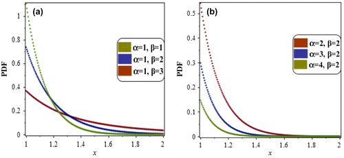
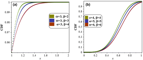
Different PDF and CDF plots of the Weibull distribution are shown in Figures 1(a–b) and 2(a–b), respectively.

Figure 1. The probability density function of Weibull distribution at various parameters choices.

Figure 2. The cumulative distribution function of Weibull distribution at various parameters choices.

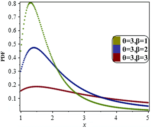
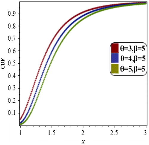
Now consider the Exponentiated Inverted Weibull distribution and it was proposed by Flaih, Elsalloukh, Mendi, and Milanova (2012). It is the generalization of the Inverted Weibull distribution and it has two shape parameters. The probability density function and cumulative distribution function (CDF) of EIWD are given by (Figures 3 and 4):(2.7) $$f(\mathit{\theta },\mathit{\beta };x)=\mathit{\theta }\mathit{\beta }{x}^{-(\mathit{\beta }+1)}{\{exp(-x^{-\mathit{\beta }})\}}^{\mathit{\theta }};\mathit{\beta }>0,\mathit{\theta }>0$$(2.7) (2.8) $$F(\mathit{\theta },\mathit{\beta };x)={\{exp(-x^{-\mathit{\beta }})\}}^{\mathit{\theta }};\mathit{\beta }>0,\mathit{\theta }>0$$(2.8)

Figure 3. PDF of the EIW distribution.

Figure 4. CDF of the EIW distribution.

The corresponding survival function, hazard rate function and reversed function are, respectively, as:(2.9) $$S(\mathit{\theta },\mathit{\beta };x)=1-{\{exp(-x^{-\mathit{\beta }})\}}^{\mathit{\theta }}$$(2.9) (2.10) $$h(\mathit{\theta },\mathit{\beta };x)=\frac{\mathit{\theta }\mathit{\beta }{x}^{-(\mathit{\beta }+1)}{\{exp(-x^{-\mathit{\beta }})\}}^{\mathit{\theta }}}{1-{\{exp(-x^{-\mathit{\beta }})\}}^{\mathit{\theta }}}$$(2.10) (2.11) $$\mathrm{\varnothing }(\mathit{\theta },\mathit{\beta };x)=\mathit{\theta }\mathit{\beta }{x}^{-(\mathit{\beta }+1)}$$(2.11)

The kth moment of the EIW distribution is given as the following:(2.12) $$\mathit{E}\mathbf{(}{\mathit{x}}^{\mathit{k}}\mathbf{)}=\underset{0}{\overset{\infty }{\int }}\mathit{\theta }\mathit{\beta }{x}^k{x}^{-(\mathit{\beta }+1)}{\{exp(-x^{-\mathit{\beta }})\}}^{\mathit{\theta }}\text{d}x$$(2.12)

Some special cases of EIWD:

EIWD has the Inverted Weibull distribution and the Exponentiated Inverted Exponential distribution as its special cases.

Hence the EIW distribution is a generality of the EIED as well as IW distribution. And some basic properties distribution is estimated through the maximum likelihood estimation method (MLE).

3. Derivation of the Length-Biased Weighted Exponentiated Inverted Weibull Distribution

In this section, we drive the LBWEIWD and also its CDF. We also drive the shape of PDF and CDF of the LBWEIWD at various choices of parametric values.

Recall the probability density function of the EIWD(3.1) $$f(x;\mathit{\theta },\mathit{\beta })=\mathit{\theta }\mathit{\beta }{x}^{-(\mathit{\beta }+1)}{\{exp(-x^{\mathit{\beta }})\}}^{\mathit{\theta }},x>0,\mathit{\theta }>0,\mathit{\beta }>0$$(3.1)

And the weight function used is as follows:(3.2) $$w(x)=x^{-c\mathit{\beta }}$$(3.2)

Substitute (3.1) and (3.2) in (2.1) then we get(3.3) $$h(x;\mathit{\beta },\mathit{\theta },c)=\frac{\mathit{\beta }{\mathit{\theta }}^{1+c}}{\mathrm{\Gamma }(1+c)}{x}^{(-c\mathit{\beta }+\mathit{\beta }+1)}{\{exp(-x^{-\mathit{\beta }})\}}^{\mathit{\theta }},x>0,\mathit{\theta }>0,\mathit{\beta }>0,c>0$$(3.3)

The density function (3.3) is known as Weighted Exponentiated Inverted Weibull Distribution.

Again substituting w(x) = x in (2.1) and using the density function of (3.3) we obtain the density function of the LBWEIWD of the form(3.4) $$g(x;\mathit{\beta },\mathit{\theta },c)=\frac{\mathit{\beta }{\mathit{\theta }}^{1+c-\frac{1}{\mathit{\beta }}}}{\mathrm{\Gamma }\left(1+c-\frac{1}{\mathit{\beta }}\right)}{x}^{-(c\mathit{\beta }+\mathit{\beta })}{\{exp(-x^{\mathit{\beta }})\}}^{\mathit{\theta }},x>0,\mathit{\beta }>0,\mathit{\theta }>0,c>0$$(3.4)

The CDF of (3.4) is defined as(3.5) $$G(\mathit{\beta },\mathit{\theta },c,x)=\frac{\mathrm{\Gamma }\left(1+c-\frac{1}{\mathit{\beta }},\frac{\mathit{\theta }}{x^{\mathit{\beta }}}\right)}{\mathrm{\Gamma }\left(1+c-\frac{1}{\mathit{\beta }}\right)}$$(3.5)

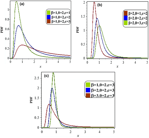
The plots of the LBWEIWD at various choices of parameters are shown in Figure 5(a–c) for comments.

Figure 5. The probability density function of LBWEIWD at various parameters choices.

Figure 5 interprets the geometric behavior of PDF of the LBWEIWD. Figures 5(a–c) depict that as the parameter c changes for representative values of the parameters $\mathit{\beta }=1,\mathit{\theta }=2$ for $c=1,2,3$, as the parameter θ changes for representative values of the parameters $\mathit{\beta }=2,c=2$ for $\mathit{\theta }=1,2,3$ and as the parameter β changes for representative values of the parameters $\mathit{\theta }=2,c=3\text{for}\mathit{\beta }=1,2,3$, respectively. We can also notice that as the values of $c,\mathit{\theta }$ and β in Figures 5(a–c), respectively, increase, the “height” of the probability density function of LBWEIWD becomes lower and the PDF is more skewed right or it can be said that the LBWEIWD is positively skewed. The increasing parameters $c,\mathit{\theta }$ and β control the shape and skewness of the density.

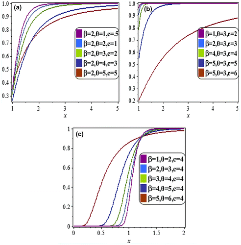
Now some plots of CDF of the LBWEIWD with specific parameter values are shown in Figure 6.

Figure 6. The cumulative distribution function of the LBWEIWD for selected values of β, θ, and c.

Figure 6 shows the different CDF plots of the LBWEIWD for various combinations of parameters. We observe that the CDF of the proposed distribution increase slowly as the values of parameters increases. All the curves given in Figure 6(a–c) approaches to 1 when $x⟶\infty$.

4. Some particular cases of LBWEIWD

This section presents some sub-models that deduced from Equation (3.4) are

Case (1): Putting $\mathit{\beta }=-\mathit{\beta },c=1/\mathit{\beta },\mathit{\theta }=\mathit{\theta }$ and multiplying by a constant (−1), the resultant distribution is Weibull distribution defined as$$g(\mathit{\beta },\mathit{\theta };x)=\mathit{\theta }\mathit{\beta }{x}^{\mathit{\beta }-1}{\{exp(-x^{-\mathit{\beta }})\}}^{\mathit{\theta }},x>0,\mathit{\beta }>0,\mathit{\theta }>0$$

Case (2): If $\mathit{\beta }=\mathit{\beta },c=\frac{1}{\mathit{\beta }},\mathit{\theta }=\mathit{\theta }$, we get Exponentiated Inverted Weibull distribution with PDF$$g(\mathit{\beta },\mathit{\theta };x)=\mathit{\theta }\mathit{\beta }{x}^{-(\mathit{\beta }+1)}{\{exp(-x^{-\mathit{\beta }})\}}^{\mathit{\theta }},x>0,\mathit{\beta }>0,\mathit{\theta }>0$$

Case (3): By substituting $\mathit{\beta }=-1,c=-1,\mathit{\theta }=\mathit{\theta }$ and multiplying by a constant (−1) then we get Exponential distribution as$$g(\mathit{\theta };x)=\mathit{\theta }{e}^{-\mathit{\theta }x},x>0,\mathit{\theta }>0$$

Case (4): In case $\mathit{\beta }=1,c=1,\mathit{\theta }=\frac{1}{\mathit{\theta }}$ reduces to$$g(\mathit{\theta };x)={\mathit{\theta }}^{-1}{x}^{-2}exp\{-{(\mathit{\theta }x)}^{-1}\},x>0,\mathit{\theta }>0$$

This density function is known in the statistics as “Inverse Exponential density function”.

Case (5): Putting $\mathit{\beta }=2,c=\frac{1}{2},\mathit{\theta }=\frac{1}{{\mathit{\theta }}^2},$ the resultant distribution is Inverse Rayleigh distribution$$g(\mathit{\theta };x)=2{\mathit{\theta }}^{-2}{x}^{-3}exp\left\{-{(\mathit{\theta }x)}^{-2}\right\},x>0,\mathit{\theta }>0$$

Case (6): Substituting $\mathit{\theta }=1,c=0,\mathit{\beta }=\mathit{\beta }$, we obtain the density function of the Length-Biased Inverted Weibull distribution$$g(\mathit{\beta };x)=\frac{\mathit{\beta }}{\mathrm{\Gamma }\left(1-\frac{1}{\mathit{\beta }}\right)}{x}^{-\mathit{\beta }}exp\{-x^{-\mathit{\beta }}\},x>0,\mathit{\beta }>1$$

Case (7): The Exponentiated inverted Exponential distribution is special case of this model when $c=1,\mathit{\beta }=1,\mathit{\theta }=\mathit{\theta },$$$g(\mathit{\theta };x)=\mathit{\theta }{x}^{-2}exp\left\{-\mathit{\theta }{x}^{-1}\right\},x>0,\mathit{\theta }>0$$

Case (8): Substituting $\mathit{\beta }=\mathit{\beta },\mathit{\theta }=\mathit{\theta },c=0,$ yields Length-Biased Exponentiated Inverted Weibull distribution$$g(\mathit{\beta },\mathit{\theta };x)=\frac{\mathit{\beta }{\mathit{\theta }}^{1-\frac{1}{\mathit{\beta }}}}{\mathrm{\Gamma }\left(1-\frac{1}{\mathit{\beta }}\right)}{X}^{-\mathit{\beta }}{\left\{exp\left(-x^{-\mathit{\beta }}\right)\right\}}^{\mathit{\theta }},x>0,\mathit{\beta }>1,\mathit{\theta }>0$$

Case (9): The case when $c=0,\mathit{\beta }=-1,\mathit{\theta }=\mathit{\theta }$ and multiplying by (−1), this model gives the Size Biased Exponential distribution (SBEPD) as$$g(\mathit{\theta };x)={\mathit{\theta }}^{2}x{e}^{-\mathit{\theta }x},x>0,\mathit{\theta }>0$$

5. The shape and mode of LBWEIWD

The shape and mode of LBWEIWD is confabulated in this section. The shape of the density function in (3.4) can be categorized by studding this function defined over the positive real line [0, ∞) and the behavior of its derivative as follows:

Limit and derivative of the function

The limit of the density function in (3.4) is as follows:(5.1) $$\underset{x\to 0}{lim}g(x;\mathit{\beta },\mathit{\theta },c)=\underset{x\to 0}{lim}\frac{\mathit{\beta }{\mathit{\theta }}^{1+c-\frac{1}{\mathit{\beta }}}}{\mathrm{\Gamma }\left(1+c-\frac{1}{\mathit{\beta }}\right)}{x}^{-(c\mathit{\beta }+\mathit{\beta })}{\{exp(-x^{-\mathit{\beta }})\}}^{\mathit{\theta }}=0$$(5.1)

(5.2) $$\underset{x\to \infty }{lim}g(x;\mathit{\beta },\mathit{\theta },c)=\underset{x\to \infty }{lim}\frac{\mathit{\beta }{\mathit{\theta }}^{1+c-\frac{1}{\mathit{\beta }}}}{\mathrm{\Gamma }\left(1+c-\frac{1}{\mathit{\beta }}\right)}{x}^{-(c\mathit{\beta }+\mathit{\beta })}{\{exp(-x^{-\mathit{\beta }})\}}^{\mathit{\theta }}=0$$(5.2)

Mode

For these limits, we conclude the PDF of the LBWEIWD when $w(x)=x^{-c\mathit{\beta }}$ and $w(x)=x$ has one mode say x₀ as follows:

(1) Taking logarithm of g(x) in (3.4) we get(5.3) $$\begin{array}{cc}log[g(x;\mathit{\beta },\mathit{\theta },c)]\hfill & =log\left[\frac{\mathit{\beta }{\mathit{\theta }}^{1+c-\frac{1}{\mathit{\beta }}}}{\mathrm{\Gamma }\left(1+c-\frac{1}{\mathit{\beta }}\right)}{x}^{-(c\mathit{\beta }+\mathit{\beta })}{\left\{exp(-x^{-\mathit{\beta }})\right\}}^{\mathit{\theta }}\right]\hfill \\ & =log\mathit{\beta }+log\mathit{\theta }+clog\mathit{\theta }-\frac{1}{\mathit{\beta }}log\mathit{\theta }-c\mathit{\beta }logx-\mathit{\beta }logx-\mathit{\theta }{x}^{-\mathit{\beta }}\hfill \\ & -log\mathrm{\Gamma }\left(1+c-\frac{1}{\mathit{\beta }}\right)\hfill \end{array}$$(5.3)

(2) Derivation for the x gives(5.4) $$\frac{\mathit{\partial }}{\mathit{\partial }x}[log(g(x;\mathit{\beta },\mathit{\theta },c)]=-\frac{c\mathit{\beta }}{x}-\frac{\mathit{\beta }}{x}+\mathit{\beta }\mathit{\theta }{x}^{-\mathit{\beta }-1}$$(5.4)

Its second derivative with respect to x is:(5.5) $$\frac{{\mathit{\partial }}^2}{\mathit{\partial }{x}^2}[log(g(x;\mathit{\beta },\mathit{\theta },c)]=-\mathit{\beta }{x}^{-2}(-c-1+\mathit{\beta }\mathit{\theta }{x}^{-\mathit{\beta }}+\mathit{\theta }{x}^{-\mathit{\beta }})<0$$(5.5)

(3) The mode of LBWEIWD is obtained by solving the non linear Equation (5.4) with respect to x and equating the first derivative to 0 leads to$$-\frac{c\mathit{\beta }}{x}-\frac{\mathit{\beta }}{x}+\mathit{\beta }\mathit{\theta }{x}^{-\mathit{\beta }-1}=0$$(5.6) $$x_0={\left[\frac{\mathit{\theta }}{1+c}\right]}^{\frac{1}{\mathit{\beta }}}$$(5.6)

Now for different values of parameters $\mathit{\beta },\mathit{\theta },$ and c the mode (x₀) of LBWEIWD is calculated and presented in Table 1.

Table 1. The mode values of LBWEIWD at various parameters combinations

β	θ	c	Mode (X0)
2	2	0.1	1.4384
2	3	0.2	1.5811
2	4	0.3	1.7541
2	5	0.4	1.8898
2	6	0.5	2.0000
3	6	0.6	1.5535
4	6	0.7	1.7306
6	6	0.8	1.2223
8	6	0.9	1.1546

6. Statistical properties of LBWEIWD

In this section, some basic properties involving moments, mean, variance, coefficient of Variation, coefficient of Skewness, and coefficient of Kurtosis, survival function, hazard rate, reversed hazard rate, and moment generating function are presented.

Moments of LBWEIWD:

If X follows the LBWEIWD with parameters β, θ, and c then kth moment of X, say ${\mathit{\mu }}_k^{\prime }$, is given as(6.1) $${\mathit{\mu }}_k^{\prime }={\mathit{\theta }}^{\frac{k}{\mathit{\beta }}}\frac{\mathrm{\Gamma }\left(1-\frac{k+1}{\mathit{\beta }}+c\right)}{\mathrm{\Gamma }\left(1+c-\frac{1}{\mathit{\beta }}\right)}$$(6.1)

From the kth moment of the LBWEIWD, the mean, variance and coefficient of Variation, Skewness (CS), and Kurtosis (CK), respectively, are as follows:(6.2) $$\mathit{\mu }=E(X)=\frac{{\mathit{\theta }}^{\frac{1}{\mathit{\beta }}}\mathrm{\Gamma }\left(1+c-\frac{2}{\mathit{\beta }}\right)}{\mathrm{\Gamma }\left(1+c-\frac{1}{\mathit{\beta }}\right)}=\frac{{\mathit{\theta }}^{\frac{1}{\mathit{\beta }}}\mathit{\delta }2}{\mathit{\delta }1}$$(6.2) (6.3) $${\mathit{\sigma }}^2=E(X^2)-{\mathit{\mu }}^2=\frac{{\mathit{\theta }}^{\frac{2}{\mathit{\beta }}}\left[\mathrm{\Gamma }\left(1+c-\frac{1}{\mathit{\beta }}\right)\mathrm{\Gamma }\left(1+c-\frac{3}{\mathit{\beta }}\right)-{\mathrm{\Gamma }}^2\left(1+c-\frac{2}{\mathit{\beta }}\right)\right]}{{\mathrm{\Gamma }}^2\left(1+c-\frac{1}{\mathit{\beta }}\right)}=\frac{{\mathit{\theta }}^{\frac{2}{\mathit{\beta }}}[\mathit{\delta }1\mathit{\delta }3-\mathit{\delta }{2}^2]}{\mathit{\delta }{1}^2}$$(6.3) (6.4) $$\text{CV}=\frac{\mathit{\sigma }}{\mathit{\mu }}=\frac{{\left[\mathrm{\Gamma }\left(1+c-\frac{1}{\mathit{\beta }}\right)\mathrm{\Gamma }\left(1+c-\frac{3}{\mathit{\beta }}\right)-{\mathrm{\Gamma }}^2\left(1+c-\frac{2}{\mathit{\beta }}\right)\right]}^{1/2}}{\mathrm{\Gamma }\left(1+c-\frac{1}{\mathit{\beta }}\right)}=\frac{{[\mathit{\delta }1\mathit{\delta }3-\mathit{\delta }{2}^2]}^{\frac{1}{2}}}{\mathit{\delta }1}$$(6.4) $$\text{CS}=\frac{{\mathit{\mu }}^3}{{\mathit{\sigma }}^3}=\frac{\left[{\mathrm{\Gamma }}^2\left(1+c-\frac{1}{\mathit{\beta }}\right)\mathrm{\Gamma }\left(1+c-\frac{4}{\mathit{\beta }}\right)-3\mathrm{\Gamma }\left(1+c-\frac{1}{\mathit{\beta }}\right)\mathrm{\Gamma }\left(1+c-\frac{2}{\mathit{\beta }}\right)\mathrm{\Gamma }\left(1+c-\frac{3}{\mathit{\beta }}\right)+2{\mathrm{\Gamma }}^3\left(1+c-\frac{2}{\mathit{\beta }}\right)\right]}{{\left[\mathrm{\Gamma }\left(1+c-\frac{1}{\mathit{\beta }}\right)\mathrm{\Gamma }\left(1+c-\frac{3}{\mathit{\beta }}\right)-{\mathrm{\Gamma }}^2\left(1+c-\frac{2}{\mathit{\beta }}\right)\right]}^{\frac{3}{2}}}$$(6.5) $$=\frac{\mathit{\delta }{1}^2\mathit{\delta }4-3\mathit{\delta }1\mathit{\delta }2\mathit{\delta }3+2\mathit{\delta }{2}^3}{{[\mathit{\delta }1\mathit{\delta }3-\mathit{\delta }{2}^2]}^{\frac{3}{2}}}$$(6.5)

$$\text{CK}=\frac{{\mathit{\mu }}^4}{{\mathit{\sigma }}^4}=\frac{\left[{\mathrm{\Gamma }}^3\left(1+c-\frac{1}{\mathit{\beta }}\right)\mathrm{\Gamma }\left(1+c-\frac{5}{\mathit{\beta }}\right)-4{\mathrm{\Gamma }}^2\left(1+c-\frac{1}{\mathit{\beta }}\right)\mathrm{\Gamma }\left(1+c-\frac{4}{\mathit{\beta }}\right)\mathrm{\Gamma }\left(1+c-\frac{2}{\mathit{\beta }}\right)+6\mathrm{\Gamma }\left(1+c-\frac{1}{\mathit{\beta }}\right)\mathrm{\Gamma }\left(1+c-\frac{3}{\mathit{\beta }}\right){\mathrm{\Gamma }}^2\left(1+c-\frac{2}{\mathit{\beta }}\right)-3{\mathrm{\Gamma }}^4\left(1+c-\frac{2}{\mathit{\beta }}\right)\right]}{{\left[\mathrm{\Gamma }\left(1+c-\frac{1}{\mathit{\beta }}\right)\mathrm{\Gamma }\left(1+c-\frac{3}{\mathit{\beta }}\right)-{\mathrm{\Gamma }}^2\left(1+c-\frac{2}{\mathit{\beta }}\right)\right]}^2}$$(6.6) $$=\frac{\mathit{\delta }{1}^3\mathit{\delta }5-\mathit{\delta }4\mathit{\delta }{1}^2\mathit{\delta }4\mathit{\delta }2+6\mathit{\delta }1\mathit{\delta }3\mathit{\delta }{2}^2-3\mathit{\delta }{2}^4}{{[\mathit{\delta }1\mathit{\delta }3-\mathit{\delta }{2}^2]}^2}$$(6.6)

Now for different values of parameters, Table 2 provided the values of the mean, variance, standard deviation (STD), coefficient of Variation (CV), coefficient of Skewness (CS), coefficient of Kurtosis (CK).

Table 2. The values of mean, variance, standard deviation (STD), coefficient of variation (CV), coefficient of skewness (CS), coefficient of kurtosis (CK) for selected β, θ, and c of LBWEIWD

β	θ	c	Mean	Var	STD	CV	CS	CK
2	1	2	0.7523	0.1008	0.3175	0.4220	3.0987	36.7035
	2	3	0.1064	0.0627	0.2504	2.7992	2.9110	12.5825
	3	4	0.0186	0.0823	0.2869	20.2814	0.1979	8.4428
	4	4	0.0381	0.0950	0.3082	20.2814	0.1979	8.4428
	5	5	0.0027	0.0621	0.2492	139.5772	0.0430	6.7715
3	1	2	0.7913	0.0385	0.1962	0.2478	1.7549	10.1447
	2	3	0.8723	0.5173	0.7192	0.2038	1.3163	6.8174
	3	4	0.9077	0.0242	0.1556	0.1715	1.0792	5.5263
	4	4	0.9946	0.0294	0.1715	0.1715	1.0792	5.5263
	5	5	0.9991	0.0233	0.1526	0.1528	0.9185	4.9078
4	1	2	0.8265	0.0214	0.1463	0.1769	1.3538	7.1935
	2	3	0.8936	0.0167	0.1292	0.1445	1.0858	5.6598
	3	4	0.9229	0.0134	0.1158	0.1252	0.9193	4.8582
	4	4	0.9918	0.0154	0.1241	0.1252	0.9193	4.8582
5	1	2	0.8527	0.0138	0.1175	0.1378	1.1600	6.6667
	2	3	0.9095	0.0107	0.1034	0.1136	0.9548	4.6447
	3	4	0.9345	0.0085	0.0922	0.0988	0.8274	4.2987
	4	4	0.9898	0.0096	0.0980	0.0988	0.8274	2.2987
6	1	2	0.8725	0.0096	0.0981	0.1123	1.1875	5.1250
	2	3	0.9218	0.0073	0.0856	0.0928	1.0445	4.0933
	3	4	0.9434	0.0058	0.0761	0.0958	1.0641	42.4791
	4	4	0.9897	0.0064	0.0799	0.0958	1.0641	42.4791
	5	5	0.9918	0.0164	0.1282	0.0722	1.8393	4.1598

Moment Generating Function:

The moment generating function (m g f) of the LBWEIWD is given by(6.7) $$M_x(t)=\sum _{r=0}^{\infty }\frac{t^r}{r!}{\mathit{\theta }}^{\frac{r}{\mathit{\beta }}}\frac{\mathrm{\Gamma }\left(1+c-\frac{r}{\mathit{\beta }}-\frac{1}{\mathit{\beta }}\right)}{\mathrm{\Gamma }\left(1+c-\frac{1}{\mathit{\beta }}\right)}$$(6.7)

Survival Function:

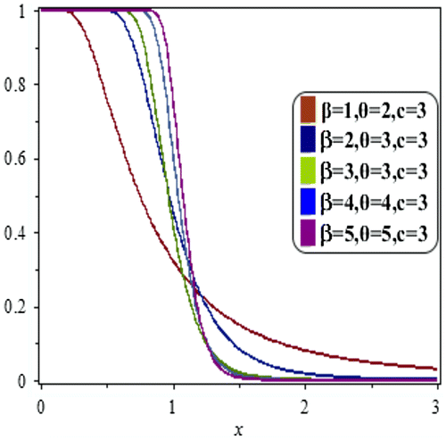
The survival function of the LBWEIWD is(6.8) $$S(x;\mathit{\beta },\mathit{\theta },c)=\frac{\mathit{\gamma }\left(1+c-\frac{1}{\mathit{\beta }},\frac{\mathit{\theta }}{x^{\mathit{\beta }}}\right)}{\mathrm{\Gamma }\left(1+c-\frac{1}{\mathit{\beta }}\right)}$$(6.8)

Table 3 and Figure 7 below presented the survival function values for various choices of parameters and X. Looking at this table we can see that the survival probability of the distribution decreases with increase in the value of parameters, for holding x. Further, from the table we can see that, for fixed c; the survival probability decreases with increase in X.

Table 3. The values of survival function of LBWEIWD at various choices of parameters

X	c	β	θ	Values
2	2	1	2	0.8647
3	2	2	2.5	0.7443
4	2	3	3	0.6640
5	2	4	3.5	0.6217
6	2	5	4	0.5965
7	2	6	4.5	0.5799
8	2	7	5	0.5681
9	2	8	5.5	0.5594
10	2	9	6	0.5526
11	2	10	6.5	0.5472
12	2	11	7	0.5429

Figure 7. The reliability function of the LBWEIWD for selected values of β, θ, and c.

Hazard Rate Function:

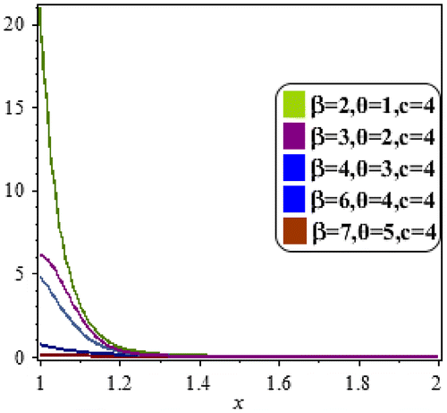
The hazard rate function of the LBWEIWD is given by(6.9) $$h(x;\mathit{\beta },\mathit{\theta },c)=\frac{\mathit{\beta }{\mathit{\theta }}^{1+c-\frac{1}{\mathit{\beta }}}{x}^{-\left(c\mathit{\beta }+\mathit{\beta }\right)}{\{exp\left(-x^{-\mathit{\beta }}\right)\}}^{\mathit{\theta }}}{\mathit{\gamma }\left(1+c-\frac{1}{\mathit{\beta }},\frac{\mathit{\theta }}{x^{\mathit{\beta }}}\right)}$$(6.9)

The hazard rate of the LBWEIWD with specific parameters values is displayed in Figure 8.

Figure 8. The hazard rate of the LBWEIWD for selected values β, θ, and c.

Reversed Hazard Rate Function:

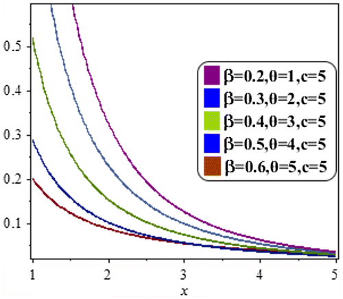
The reversed hazard rate function of the LBWEIWD is given by(6.10) $$\mathrm{\varnothing }\left(x;\mathit{\beta },\mathit{\theta },c\right)=\frac{\mathit{\beta }{\mathit{\theta }}^{1+c-\frac{1}{\mathit{\beta }}}{x}^{-(c\mathit{\beta }+\mathit{\beta })}exp\{-\mathit{\theta }{x}^{-\mathit{\beta }}\}}{\mathrm{\Gamma }\left(1+c-\frac{1}{\mathit{\beta }},\frac{\mathit{\theta }}{x^{\mathit{\beta }}}\right)}$$(6.10)

The plot of reversed hazard rate with specific parameter values is made in Figure 9.

Figure 9. The reversed hazard rate of the LBWEIWD for selected values of β, θ, and c.

7. Parameter estimation

In this section estimation of the three parameters $\mathit{\beta },\mathit{\theta }$ and c of Length-Biased Weighted Exponentiated Inverted Weibull Distribution are obtained by the method of moments and maximum likelihood method:

Method of moments (MOM)

This procedure follows by equating the population moments to the sample moments then we have the system of three equations;(i) $$\frac{1}{n}\sum _{i=1}^{n}X=\frac{{\mathit{\theta }}^{\frac{1}{\mathit{\beta }}}\mathrm{\Gamma }\left(1+c-\frac{2}{\mathit{\beta }}\right)}{\mathrm{\Gamma }\left(1+c-\frac{1}{\mathit{\beta }}\right)}$$(i) (ii) $$\frac{1}{n}\sum _{i=1}^n{X}_i^2=\frac{{\mathit{\theta }}^{\frac{2}{\mathit{\beta }}}\mathrm{\Gamma }\left(1+c-\frac{3}{\mathit{\beta }}\right)}{\mathrm{\Gamma }\left(1+c-\frac{1}{\mathit{\beta }}\right)}$$(ii) (iii) $$\frac{1}{n}\sum _{i=1}^n{X}_i^3=\frac{{\mathit{\theta }}^{\frac{3}{\mathit{\beta }}}\mathrm{\Gamma }\left(1+c-\frac{4}{\mathit{\beta }}\right)}{\mathrm{\Gamma }\left(1+c-\frac{1}{\mathit{\beta }}\right)}$$(iii)

Solving the system (i), (ii), and (ii), the moment’s estimates of $\mathit{\beta },\mathit{\theta }$ and c can be determined. These approximations are mostly used as initial values for the MLE procedure when no closed form exists for the MLE and normal equations need to be resolved iteratively.

Maximum-likelihood estimators (MLE)

Let suppose that sample was drawn from (3.4) and we drive the non linear equations for finding the maximum likelihood estimators of the parameters. It is assumed that X follows LBWEIWD (β, θ, c) and (β, θ, c)^T denotes the parameter vector. The estimation of the parameters for the LBWEIWD is done via the MLE; we will provide the MLE procedure as follows:

The likelihood function $L(\mathit{\beta },\mathit{\theta },c;x)$ of the LBWEIWD $\left(\mathit{\beta },\mathit{\theta },\text{and}c\right),$ and then find the value of $\mathit{\beta },\mathit{\theta },$ and c which maximize $L(\mathit{\beta },\mathit{\theta },c;x)$ is given by(7.1) $$L(\mathit{\beta },\mathit{\theta },c;x)=\frac{{\mathit{\beta }}^n{\mathit{\theta }}^{n\left(1+c-\frac{1}{\mathit{\beta }}\right)}}{{\left[\mathrm{\Gamma }\left(1+c-\frac{1}{\mathit{\beta }}\right)\right]}^n}{\mathrm{\Pi }}_{i=1}^n{x}_i^{-(c\mathit{\beta }+\mathit{\beta })}exp\left\{-\mathit{\theta }\sum _{i=1}^n{x}_i^{-\mathit{\beta }}\right\}$$(7.1)

The log likelihood function of n observations of X can be written as$$l(\mathit{\beta },\mathit{\theta },c;X)=logL(\mathit{\beta },\mathit{\theta },c;X)$$$$=nlog\mathit{\beta }+nlog\mathit{\theta }+nclog\mathit{\theta }-\frac{n}{\mathit{\beta }}log\mathit{\theta }-(c\mathit{\beta }-\mathit{\beta })\sum _{i=1}^{n}log{X}_i-\mathit{\theta }\sum _{i=1}^n{X}_i^{-\mathit{\beta }}-nlog\mathrm{\Gamma }\left(1+c-\frac{1}{\mathit{\beta }}\right)$$(7.2) $$=nlog\mathit{\beta }+nlog\mathit{\theta }+nclog\mathit{\theta }-\frac{n}{\mathit{\beta }}log\mathit{\theta }-c\mathit{\beta }\sum _{i=1}^{n}logX-\mathit{\beta }\sum _{i=1}^{n}log{X}_i-\mathit{\theta }\sum _{i=1}^n{X}_i^{-\mathit{\beta }}-nlog\mathrm{\Gamma }\left(1+c-\frac{1}{\mathit{\beta }}\right)$$(7.2)

Differentiating (7.2) with respect to $\mathit{\beta },\mathit{\theta }$ and c, respectively, as follows:(7.3) $$\frac{\mathit{\partial }l}{\mathit{\partial }\mathit{\beta }}=\frac{n}{\mathit{\beta }}+\frac{nln(\mathit{\theta })}{{\mathit{\beta }}^2}-c\left[\sum _{i=1}^{n}ln{(X)}_i\right]-\left[\sum _{i=}^n(X)\right]-\mathit{\theta }\left[\sum _{i=1}^n(-X_i^{-\mathit{\beta }}\text{ln}(X_i))\right]-\frac{n\mathit{\phi }\left(1+c-\frac{1}{\mathit{\beta }}\right)}{{\mathit{\beta }}^2}$$(7.3) (7.4) $$\frac{\mathit{\partial }l}{\mathit{\partial }\mathit{\theta }}=\frac{n}{\mathit{\theta }}+\frac{nc}{\mathit{\theta }}-\frac{n}{\mathit{\beta }\mathit{\theta }}-\left[\sum _{i=1}^n{X}_i^{-\mathit{\beta }}\right]$$(7.4)

(7.5) $$\frac{\mathit{\partial }l}{\mathit{\partial }c}=nln(\mathit{\theta })-\mathit{\beta }\left[\sum _{i=1}^n\text{ln}(X_i)\right]-n\mathit{\phi }\left(1+c-\frac{1}{\mathit{\beta }}\right)$$(7.5)

Solving the Equation (7.3) $\frac{\mathit{\partial }logL(X_1,X_2\dots X_n,\mathit{\beta },\mathit{\theta },c)}{\mathit{\partial }\mathit{\beta }}=0$ yields the maximum likelihood(7.6) $$\frac{n}{\mathit{\beta }}+\frac{nln(\mathit{\theta })}{{\mathit{\beta }}^2}-c\left[\sum _{i=1}^{n}ln(X_i)\right]-\left[\sum _{i=}^{n}ln(X_i)\right]-\mathit{\theta }\left[\sum _{i=1}^n(-X_i^{-\mathit{\beta }}\text{ln}(X_i))\right]-\frac{n\mathit{\phi }\left(1+c-\frac{1}{\mathit{\beta }}\right)}{{\mathit{\beta }}^2}=0$$(7.6)

Solving the Equation (7.4) $\frac{\mathit{\partial }logL(X_1,X_2\dots X_n,\mathit{\beta },\mathit{\theta },c)}{\mathit{\partial }\mathit{\theta }}=0$ yields the maximum likelihood (7.7) $$\frac{n}{\mathit{\theta }}+\frac{nc}{\mathit{\theta }}-\frac{n}{\mathit{\beta }\mathit{\theta }}-\left[\sum _{i=1}^n{X}_i^{-\mathit{\beta }}\right]=0$$(7.7)

Solving the Equation (7.5) $\frac{\mathit{\partial }logL(X_1,X_2\dots X_n,\mathit{\beta },\mathit{\theta },c)}{\mathit{\partial }c}=0$ yields the maximum likelihood(7.8) $$Nln(\mathit{\theta })-\mathit{\beta }\left[\sum _{i=1}^n\text{ln}(X_i)\right]-n\mathit{\phi }\left(1+c-\frac{1}{\mathit{\beta }}\right)=0$$(7.8)

To find out the likelihood estimators of $\mathit{\beta },\mathit{\theta }$ and c, we have to resolve the given system of non linear Equations (7.6)–(7.8) with respect to $\mathit{\beta },\mathit{\theta }$ and c but the non linear Equations (7.6)–(7.8) do not seem to have a closed form solution and must be solved iteratively to gain the estimate of the parameters or the system of the three equations can be solved consecutively. We take the MLE $\mathit{\beta }\widehat{},\mathit{\theta }\widehat{}\text{and}c\widehat{}$, respectively, by resolving iteratively to zero. These equations are not in closed form and we can apply a numerical technique to attain the expectation of them, such as Newton-Raphson method to obtain the solution.

Table 4. Distance between cracks in a pipe data-set

30.94	18.51	16.62	51.56	22.85	22.38	19.08	49.56
17.12	10.67	25.43	10.24	27.47	14.70	14.10	29.93
27.98	36.02	19.40	14.97	22.57	12.26	18.14	18.84

Example

As in Section 8, we consider uncensored data on distance between cracks in a pipe data-set given in Table 4.The data can be modeled by LBWEIWD and also we estimate the parameters $\mathit{\beta },\mathit{\theta }$ and c using Newton-Raphson method for simultaneously three equations, by taking the initial estimate $\mathit{\beta }\widehat{}$ = 0.5, $\mathit{\theta }\widehat{}$ = 2, and $c\widehat{}$ = 1.5 then the estimate of values are: $\mathit{\beta }\widehat{}$ = 1.4256, $\mathit{\theta }\widehat{}$ = 100.7943, $c\widehat{}$ = 1.4857.

8. Data analysis

This section presents the comparison analysis of the LBWEIW, LBEIW, and EIW distributions applying to the real data-sets. We consider uncensored data on distance between cracks in a pipe data-set. The data is given in Table 4. We can also perform formal goodness-of-fit test in order to verify which distribution fits to the data. We apply the Kolmogorov-Smirnov test (KS test) for the goodness-of-fit purpose.

Table 5 lists the MLE estimates of the parameters β, θ, and c values of the test statistics which is KS test. The p-value of KS for the LBWEIWD is 0.9388. The results in Table 5 showed that the LBWEIWD fits the data as well as LBIW, Weibull, LBEIW, and EIW distribution. In fact, based on the value of the KS-statistic, we observe that the LBWEIWD provides the best fit for this data among all the models considered. So it is evident that the LBWEIWD is the best distribution and is a strong competitor to other distributions commonly used in literature for fitting lifetime data as given below.

Table 5. Goodness-of- fit summary of distance between cracks in a pipe data-set.

Fitting	KS test		Estimate
Distribution	Statistic	p-value	β	θ	c
LBWEIW	0.1021	0.9388	1.4256	100.7943	1.4857
LBIW	0.5129	0.0000	1.3484	–	–
Weibull	0.1436	0.6532	2.3089	26.0230	–
LBEIW	0.1031	0.9376	3.3891	9508.9505	–
EIW	0.0891	0.9822	2.7347	2384.5601	–

9. Conclusions

In this article, the Length-Biased version of weighted Exponentiated inverted Weibull distribution is introduced. A new three parameter distribution is proposed. At first the PDF of the weighted Exponentiated inverted Weibull distribution has been obtained considering weight as $w(x)=x^{-c\mathit{\beta }}$ then from PDF of WEIWD, LBWEIWD have been obtained considering weight as w(x) = x. Next to characterize the distribution of random variable x of LBWEIWD, three functions have been introduced namely survival function or mass function and the failure rate function or hazard function. The moment’s coefficient of variation coefficient of skewness coefficient or kurtosis of LBWEIWD has been derived, for estimation of parameters of LBWEIWD the maximum likelihood estimators have been used.

An application of this new model to real data-set on distance between crakes in a pipe is given to demonstrate that these can be used quite efficaciously to stipulate improved fits than other available models that might be of use for practitioners in the applied sciences and this shows that the fit of the LBWEIWD is the best fit to the data with highest p-value. We hope that this provides a rather general and flexible framework for statistical analysis and may attract the extensive application in life time data analysis and other fields.

Additional information

Funding

Funding. The authors received no direct funding for this research.

Notes on contributors

Aamir Saghir

Aamir Saghir obtained his PhD degree in Statistics from the Department of Mathematics, Zhejiang University, Hangzhou, China, under CSC program. He is currently working in Mirpur University of Science and Technology (MUST), Mirpur, Pakistan, as a senior lecturer. His research interests include Statistical Quality Control, Mathematical Statistics, and Applied Statistics.

Sadaf Tazeem

Sadaf Tazeem obtained her MPhil degree in Mathematics from the Department of Mathematics, Mirpur University of Science and Technology (MUST), Mirpur AJK. She is currently doing her PhD from Mirpur University of Science and Technology (MUST), Mirpur, Pakistan. Her research interests include Mathematical Statistics and probability theory.

Ishfaq Ahmad

Ishfaq Ahmad obtained his PhD degree in Statistics. He is currently working as an assistant professor in Department of Mathematics and Statistics in International Islamic University Islamabad, Pakistan. His research interests include Mathematical Statistics, Applied Statistics and Theory of estimation.

References

- Ahmad, A., & Ahmad, S. P. (2014). Characterization and estimation of double weighted Rayleigh distribution. Journal of Agriculture and Life Sciences, 1, 2375–4214.
- Aleem, M., Sufyan, M., & Khan, N. S. (2013). A class of modified weighted Weibull distribution and its properties. American Review of Mathematics and Statistics, 1, 29–37.
- Al-Kadim, K., & Hantoosh, A. F. (2013). Double weighted distribution & double weighted exponential distribution. Mathematical Theory and Modeling, 3, 2224–5804.
- Al-Kadim, K. A., & Hantoosh, A. F. (2014). Double weighted inverse Weibull Distribution. Pakistan Publishing Group, 978- 969-9347-16-0.
- Al-Khadim, A. K., & Hussein, A. N. (2014). New proposed length-biased weighted Exponential and Rayleigh distribution with application. Mathematical Theory and Modeling, 4, 2224–5804.
- Alqallaf, F., Ghitany, M. E., & Agostinelli, C. (2015). Weighted exponential distribution: Different methods of estimations. Applied Mathematics & Information Sciences, 9, 1167–1173.
- Asgharzadeh, A., Bakouch, H. S., Nadarajah, S., & Sharafi, F. (2016). A new weighted Lindley distribution with application. Brazilian Journal of Probability and Statistics, 30(1), 1–27.10.1214/14-BJPS253
- Badmus, N., Bamiduro, T. A., & Ogunobi, S. G. (2014). Lehmann type II weighted Weibull distribution. International Journal of Physical Sciences, 9, 71–78.
- Badmus, N. I., Bamiduro, A. T., Animasaun, M. A. R., & Akingbade, A. A. (2015). Beta weighted exponential distribution: Theory and application. International Journal of Mathematical Analysis and Optimization: Theory and Applications, 1, 55–66.
- Bashir, S., & Rasul, M. (2015). Some properties of the Weighted Lindley distribution. International Journal of Economic and Business Review, 3, 0187–2349.
- Berrettoni, J. N. (1964). Practical applications of the Weibull distribution. Industrial Quality Control, 21, 71–79.
- Cox, D. R. (1962). Renewal Theory. New York, NY: Barnes & Noble.
- Das, K. K., & Roy, T. D. (2011a). Applicability of length biased generalized Rayleigh distribution. Advances in Applied Science Research, 2, 320–327.
- Das, K. K., & Roy, T. D. (2011b). On some length-biased weighted Weibull distribution. Advances in Applied Science Research, 2, 465–475.
- Del Castillo, J. D., & Pérez-Casany, M. P. (1998). Weighted Poisson distributions for overdispersion and underdispersion situations. Annals of the Institute of Statistical Mathematics, 50, 567–585.10.1023/A:1003585714207
- El-Shaarawi, A., Walter, W. P., & Patil, G. P. (2002). Weighted distribution. Encyclopedia of Environmetics, 4, 2369–2377.
- Farahani, Z. S. M., & Khorram, E. (2014). Bayesian statistical inference for weighted exponential distribution. Journal of Statistical Computation and Simulation, 43, 0361–0918.
- Fay, D., Haddadi, H., Uhlig, S., Moore, A. W., Mortier, R., & Jamakovic, A. (2008). Weighted spectral distribution (Technical Report UCAM-CL-TR-729, pp. 1476–2986). Cambridge.
- Fisher, R. A. (1934). The effect of methods of ascertainment upon the estimation of frequencies. Annals of Eugenics, 6, 13–25.10.1111/j.1469-1809.1934.tb02105.x
- Flaih, A., Elsalloukh, H., Mendi, E., & Milanova, M. (2012). The exponentiated inverted Weibull distribution. Applied Mathematics & Information Sciences, 6, 167–171.
- Ghitany, E., & Al-Mutairi, D. K. (2008). Size-biased Poisson-Lindley distribution and its application. METRON-International Journal of Statistics, 3, 299–311.
- Ghitany, M. E., Al-Mutairi, D. K., & Husain, H. A. (2011). A two-parameter weighted Lindley distribution and its applications to survival data. Mathematics and computers in Simulation, 81, 11901201.
- Gupta, P. L., & Tripathi, R. C. (1990). Effect of length-biased sampling on the modeling error. Communications in Statistics - Theory and Methods, 19, 1483–1491.10.1080/03610929008830274
- Gupta, R. C., & Keating, J. P. (1985). Relations for reliability measures under length biased sampling. Scandanavian Journal of Statistics, 13, 49–56.
- Gupta, R. C., & Kirmani, S. N. U. A. (1990). The role of weighted distributions in Stochastic modeling. Communications in statistics –Theory and Methods, 19, 3147–3162.
- Gupta, R. D., & Kundu, D. A. (2009). A new class of weighted exponential distributions. Statistics, 43, 621–634.10.1080/02331880802605346
- Idowu, B. N., & Adebayo, B. T. (2014). Some statistical properties of exponentiated weighted Weibull distribution. Global Journal of Science Frontier Research: F Mathematics and Decision Sciences, 14, 0975–5896.
- Kao, J. H. K. (1959). A graphical estimation of mixed Weibull parameters in life-testing of electron tubes. Technometrics, 1, 389–407.10.1080/00401706.1959.10489870
- Kersey, J. X. (2010). Weighted inverse Weibull and beta-inverse Weibull distribution (MSC Thesis). University of Georgia Southern, Statesboro.
- Khattree, R. (1989). Characterization of inverse-Gaussian and gamma distributions through their length-biased distributions. IEEE Transactions on Reliability, 38, 610–611.10.1109/24.46490
- Mahdavi, A. (2015). Two weighted distributions generated by exponential distribution. Journal of Mathematical Extension, 9(1), 1–12.
- Mahdy, M. (2011). A weighted gamma distribution and its properties. Journal of Economic Quality Control, 26, 133–144.
- Mizaal, A. R. (2015). Mathematical study of weighted two parameters exponential distribution. Education College, Al – Mustansryia University, 93, 0215–9511.
- Modi, K. (2015). Length-biased Weighted Maxwell distribution. Pakistan Journal of Statistics and Operation Research, 11, 465–472.10.18187/pjsor.v11i4.1008
- Nanuwong, N., & Bodhisuwan, W. (2014). Length biased beta-pareto distribution and its structural properties with application. Journal of Mathematics and Statistics, 10, 49–57.10.3844/jmssp.2014.49.57
- Nasiru, S. (2015). Another weighted Weibull distribution from Azzalini’s family. European Scientific Journal, 11, 1857–7881.
- Odubote, O., & Oluyede, B. O. (2014). Theoretical properties of the weighted Feller- Pareto and related distributions. Asian Journal of Mathematics and Applications, 2014, 2307–7743.
- Oguntunde, P. E. (2015). On the exponentiated weighted exponential distribution and its basic statistical properties. Applied Science Reports, 10, 160–167.
- Oluyede, B. O. (1999). On inequalities and selection of experiments for length-biased distributions. Probability in the Engineering and Informational Sciences, 13, 169–185.
- Oluyede, B. O., & George, E. O. (2000). On stochastic inequalities and comparisons of reliability measures for weighted distributions. Mathematical Problems in Engineering, 8(1), 1–13.
- Patil, G. P., & Ord, J. K. (1976). On size-biased sampling and related form-invariant weighted distributions. Sankhya - The Indian Journal of Statistics, 38, 48–61.
- Patil, G. P., & Rao, C. R. (1978). Weighted distributions and size-biased sampling with applications to wildlife populations and human families. Biometrics, 34, 179–189.10.2307/2530008
- Priyadarshani, H. A. (2011). Statistical properties of weighted generalized Gamma distribution (MSC Thesis). University of Georgia Southern, Statesboro.
- Ramadan, M. M. (2013). A class of weighted Weibull distribution and its properties. Studies in Mathematical Sciences, 6, 35–45.
- Rao, C. R. (1965). On discrete distributions arising out of methods of ascertainment. In G. P. Patil (Ed.), Classical and contagious discrete distributions (pp. 320–332). Calcutta: Pergamon Press and Statistical Publishing Society.
- Ratnaparkhi, M. V., & Naik -Nimbalkar, U. V. (2012). The length-biased lognormal distribution and its application in the analysis of data from oil field exploration studies. Modern Applied Statistical Methods, 11, 225–260.
- Roman, R. (2010). Theoretical properties and estimation in weighted Weibull and related distributions (Electronic Theses and Dissertations). University of Georgia Southern, Statesboro.
- Saghir, A., Saleem, M., Khadim, A., & Tazeem, S. (2015). The modified double weighted exponential distribution with properties. Mathematical Theory and Modeling, 5, 2224–5804.
- Seenoi, P., Supapa, K. T., & Bodhisuwan, W. (2014). The length biased exponentiated inverted Weibull Distribution. International Journal of Pure and Applied Mathematics, 92, 191–206.
- Shakhatreh, M. K. (2012). A two-parameter of weighted exponential distributions. Statistics & Probability Letters, 82, 252–261.10.1016/j.spl.2011.10.008
- Sherina, V., & Oluyede, B. O. (2014). Weighted inverse Weibull distribution: Statistical properties and applications. Theoretical Mathematics & Applications, 4(2), 1–30.
- Shi, X., Broderick, O., & Pararai, M. (2012). Theoretical properties of weighted generalized Rayleigh and related distributions. Applied Mathematical Sciences, 2, 45–62.
- Weibull, W. (1951). A statistical distribution functions of wide applicability. Applied Mechanics, 18, 293–297.
- Ye, Y., Oluyede, B. O., & Pararai, M. (2012). Weighted generalized beta distribution of the second kind and related distributions. Journal of Statistical and Econometric Methods, 1, 13–31.
- Zelen, M., & Feinleib, M. (1969). On the theory of screening for chronic diseases. Biometrika, 56, 601–614.10.1093/biomet/56.3.601