Analytical solutions of a time-fractional nonlinear transaction-cost model for stock option valuation in an illiquid market setting driven by a relaxed Black–Scholes assumption

Abstract

In financial mathematics, trading in an illiquid market has become a topic of great concern since assets in such market cannot be sold easily for cash without at least a minimal loss of value. This may be due to uncertainty traceable to factors like lack of interested buyers, transaction cost, and so on. Here, we obtain analytical solutions of a time-fractional nonlinear transaction-cost model for stock option valuation in an illiquid market through a relatively new semi-analytical method: modified differential transform method. Firstly, we considered a nonlinear option pricing model obtained when the constant volatility assumption of the classical linear Black–Scholes option pricing model is relaxed by including transaction cost. Thereafter, we extend, for the first time in literature, this nonlinear option pricing model to a time-fractional ordered form, and obtain approximate-analytical solutions to this new nonlinear model via the proposed technique. For efficiency and reliability of the method, two cases with five examples are considered: case 1 with two examples for time-integer order, and case 2 with three examples for time-fractional order. Our results strongly agree with the associated exact solutions in literature and those obtained via the application of Adomian Decomposition Method (ADM) even though our approximate solutions include only terms up to time power two, accuracy is improved for more terms. This therefore, shows that the result obtained via the ADM is a particular case of this present work when α = 1. Maple 18 software is used for the computations done in this work.

Keywords:

• fractional calculus
• nonlinear Black–Scholes model
• illiquid market
• option pricing
• MDTM

Mathematics subject classification:

• 26A33
• 34G20
• 91G80

Public Interest Statement

Liquidity is a term used in finance to describe the degree to which an underlying asset can be easily sold or bought in the market setting in a way that the asset’s price is not affected. This is unlike an illiquid market where the trading assets cannot be exchanged for cash easily without a remarkable reduction in the price due to uncertainty. This therefore requires an optimal model. The classical Black–Scholes model fits in for such option trading but for some of its assumptions such as the constant nature of the drift and volatility parameters. Addressing this leads to a nonlinear option pricing model extended to time-fractional form and solved for approximate-analytical solutions via a proposed semi-analytical method.

1. Introduction

The term “liquidity” is used in describing the degree to which an underlying asset can be easily exercised (sold or bought) in the market setting in a way that the asset’s price is not affected (Acharya & Pedersen, 2005; Amihud & Mendelson, 1986). Money or cash is an example of liquid assets because it can be sold for items such as goods and services (instantly) with (or without minimal) loss of value. A liquid market is mainly described by ever ready and willing investors. However, in an illiquid market, the concerned assets cannot be sold or exchanged for cash easily without a remarkable reduction in the price due to uncertainty such as lack of interested buyers and transaction cost, to mention but a few (Keynes, 1971). Stock option is a good example of an illiquid asset.

The standard Black–Scholes model is a very vital tool in modern finance and option theory (Black & Scholes, 1973). Nevertheless, most of the assumptions under which this pricing model is formulated appear not realistic in practical settings. These assumptions include: the asset price S following a Geometric Brownian motion (GBM), constant drift parameter μ, constant volatility rate σ, lack of arbitrage opportunities (lack of risk-free profit), frictionless, and competitive markets (Edeki & Ugbebor, 2015; González-Gaxiola, Ruíz de Chávez, & Santiago, 2015). In a competitive market, there are no transaction costs (say taxes), and restrictions on trade are not honoured (say short sale constraints) (Cetin, Jarrow, & Protter, 2004), whereas in a competitive market, a trader is unbound to buy or sell any amount of a security without price alteration.

Based on these assumptions, the stock price S, at time t (0 < t < T) follows the stochastic differential equation (SDE):(1.1) $$\frac{\text{d}S}{S}=\mathit{\mu }\text{d}t+\mathit{\sigma }\text{d}{W}_t$$(1.1)

where μ represents mean rate of return of S, σ is the volatility parameter, and W_t is a standard Brownian motion. Therefore, for an option value u = u(s, t), we have:(1.2) $$u_t+rS{u}_{\text{S}}+\frac{1}{2}{S}^2{\mathit{\sigma }}^2{u}_{\text{SS}}=ru$$(1.2)

where $u_{\overline{\mathit{\omega }}}$ indicates partial derivative of u w.r.t. the subscripted variable $\overline{\mathit{\omega }}$, while $u(0,t)=0,u(s,t)\to 0\text{as}S\to \infty u\left(s,T\right)={\left(S-E\right)}^{+}$, E is a constant.

In literature, a lot of models with regard to volatility have been proposed for option pricing. However, the simplest of such adopts constant volatility, whereas constant volatility cannot fully explain observed market prices for options valuation except when modified (Barles & Soner, 1998; Boyle & Vorst, 1992; Edeki, Owoloko, & Ugbebor, 2016; Edeki, Ugbebor, & Owoloko, 2016).

Many researchers have considered solving (1.2) for approximate solutions using direct, analytical, or semi-analytical methods (Allahviranloo & Behzadi, 2013; Ankudinova & Ehrhardt, 2008; Bohner & Zheng, 2009; Cen & Le, 2011; Company, Navarro, Ramón Pintos, & Ponsoda, 2008; Edeki, Ugbebor, & Owoloko, 2015; Jódar, Sevilla-Peris, Cortés, & Sala, 2005; Rodrigo & Mamon, 2006). The notion of liquidity is therefore introduced when the frictionless and the competitive markets’ assumptions are relaxed, thereby giving rise to a nonlinear version of the Black–Scholes model (as a result of transaction cost involvement) (Bakstein & Howison, 2003). Bakstein and Howison (2003) see liquidity as a combination of trader’s individual transaction cost and a price slippage impact. It is therefore, our intention to obtain analytical solutions of the time-fractional nonlinear transaction cost model for stock prices in an illiquid market (Bakstein and Howison model (Bakstein & Howison, 2003)).

Recently, significant attention has been given to the study of fractional differential equations (FDEs) with their wider applications because fractional calculus seems to be a generalization of the conventional calculus (He, 1999). The ultimate benefit of the FDEs lies in their properties of non-locality since integer order differential operators are local operators while fractional order differential operators are nonlocal, signifying that the next state of a system depends not only on its current state but also on all of its historical states (Miller & Ross, 1993; Podlubny, 1999). Recent works on FDEs include those of (Edeki, Akinlabi, & Adeosun, 2016a; Ibis, Bayram, & Agargun, 2011; Kilbas, Srivastava, & Trujilo, 2006; Mokhtary, Ghoreishi, & Srivastava, 2016; Song, Yin, Cao, & Lu, 2013).

In considering the solutions of linear time-fractional Black–Scholes Equations (LTFBSEs) in option pricing and valuation; Elbeleze, Kilicman, and Taib (2013) consider the application of the Homotopy Perturbation Sumudu Transform (HPSTM), Kumar et al. (2012) combine the homotopy perturbation method with Laplace transform. Ghandehari and Ranjbar (2014) extend the decomposition method through expansion series. Kumar, Kumar, and Singh (2014) apply the HPM and HAM to solve the time-fractional Black–Scholes (TFBSE) with boundary conditions. Ahmad, Shakeel, Hassan, and Mohyud-Din (2013) employ fractional variation iterative method to obtain analytical solutions of linear fractional Black–Scholes equations. Hariharan (2013) use the Laplace Legendre wavelet method for numerical solutions. Recently, Ravi Kanth and Aruna (2016) present fractional differential transform method (FDTM) and its modified form (MFDTM) for the solution of time- fractional B-S European option pricing equation while Khan and Ansari (2016) consider same by means of sumudu transform method (STM).

In this present work, a modified version of the DTM called projected/modified differential transform method (MDTM) is adopted and presented for the first time, for analytical solutions of a time-fractional nonlinear transaction-cost model for stock option valuation in an illiquid market setting driven by a relaxed Black–Scholes model assumption. We also remark here, to the best of our knowledge, that this is the first time such nonlinear option pricing model is extended to time-fractional order type.

The remaining part of the paper is structured as follows: in Section 2, we give a brief note on the nonlinear option pricing model; in Section 3, we present an overview, the basic theorems of the semi-analytical method and the analysis of its fractional form; in Section 4, the MDTM is applied to the time-fractional order-type nonlinear option pricing model (in its general form) followed by numerical examples for some special cases with graphical interpretations; in Section 5, we give concluding remarks and summary of our results.

2. Bakstein and Howison equation: nonlinear Black–Scholes option pricing model

In this section, consideration will be on a situation where both μ (the drift parameter), and σ (the volatility parameter) can be function of time τ, stock price S and the derivatives of the option price Λ. In particular, the non-constant volatility function of the form:(2.1) $$\mathit{\sigma }=\widehat{\mathit{\sigma }}\left(\mathit{\tau },S,\frac{\mathit{\partial }\mathrm{\Lambda }}{\mathit{\partial }S},\frac{{\mathit{\partial }}^2\mathrm{\Lambda }}{\mathit{\partial }{S}^2}\right)$$(2.1)

is to be considered. Thus, (2.1) in (1.2) yields:(2.2) $$\frac{\mathit{\partial }\mathrm{\Lambda }}{\mathit{\partial }\mathit{\tau }}+rS\frac{\mathit{\partial }\mathrm{\Lambda }}{\mathit{\partial }S}+\frac{1}{2}{S}^2{\widehat{\mathit{\sigma }}}^2\left(\mathit{\tau },S,\frac{\mathit{\partial }\mathrm{\Lambda }}{\mathit{\partial }S},\frac{{\mathit{\partial }}^2\mathrm{\Lambda }}{\mathit{\partial }{S}^2}\right)\frac{{\mathit{\partial }}^2\mathrm{\Lambda }}{\mathit{\partial }{S}^2}-r\mathrm{\Lambda }=0.$$(2.2)

The model Equation (1.2) can be improved upon via (2.1) in the line of transaction costs inclusion. As such, the approach of (Frey & Patie, 2002; Frey & Stremme, 1997) will be followed for the effects on the price with the result:(2.3) $$\mathit{\sigma }=\widehat{\mathit{\sigma }}\left(\mathit{\tau },S,\frac{\mathit{\partial }\mathrm{\Lambda }}{\mathit{\partial }S},\frac{{\mathit{\partial }}^2\mathrm{\Lambda }}{\mathit{\partial }{S}^2}\right)\left(1-\mathit{\rho }S\mathit{\lambda }(S)\frac{{\mathit{\partial }}^2\mathrm{\Lambda }}{\mathit{\partial }{S}^2}\right)$$(2.3)

where σ indicates the traditional volatility, ρ is a constant measuring the liquidity of the market, and λ represents the price of risk (Bakstein & Howison, 2003).

With the assumption that the price of risk is unity (a special case: where λ(S) = 1), and a little algebra with the notion that 1 ≈ (1 – f^*)² (1 + 2f^* + O(f^*)³), one can therefore write (2.2) as:(2.4) $$\frac{\mathit{\partial }\mathrm{\Lambda }}{\mathit{\partial }\mathit{\tau }}+rS\frac{\mathit{\partial }\mathrm{\Lambda }}{\mathit{\partial }S}+\frac{1}{2}{S}^2\left[{\mathit{\sigma }}^2\left(1+2\mathit{\rho }S\frac{{\mathit{\partial }}^2\mathrm{\Lambda }}{\mathit{\partial }{S}^2}\right)\right]\frac{{\mathit{\partial }}^2\mathrm{\Lambda }}{\mathit{\partial }{S}^2}-r\mathrm{\Lambda }=0$$(2.4)

such that Λ(S, T) = h(S), $S\in$ [0,∞). Letting t + τ = T and w(S, t) = Λ(S, τ), Equation (2.4) thus becomes:(2.5) $$\frac{\mathit{\partial }w}{\mathit{\partial }t}+rS\frac{\mathit{\partial }w}{\mathit{\partial }S}+\frac{1}{2}{S}^2{\mathit{\sigma }}^2\left(1+2\mathit{\rho }S\frac{{\mathit{\partial }}^{2}w}{\mathit{\partial }{S}^2}\right)\frac{{\mathit{\partial }}^{2}w}{\mathit{\partial }{S}^2}=rw,w\left(S,0\right)=h\left(S\right).$$(2.5)

The exact solution of (2.5) according to (Esekon, 2013) is of the form:(2.6) $$w\left(S,t\right)=S-{\mathit{\rho }}^{-1}\sqrt{S_0}\left(\sqrt{S}exp\left(\frac{4r+{\mathit{\sigma }}^2}{8}\right)t+\frac{\sqrt{S_0}}{4}exp\left(\frac{4r+{\mathit{\sigma }}^2}{4}\right)t\right).$$(2.6)

For σ, S₀, S, |ρ| > 0, w(S, t) = w, while r, t ≥ 0, S₀ as an initial stock price, with:(2.7) $$w\left(S,0\right)={\left(S-{\mathit{\rho }}^{-1}\left(\sqrt{S_{0}S}+\frac{S_0}{4}\right)\right)}^{+}.$$(2.7)

Liu and Yong (2005) considered and established the existence and uniqueness of this nonlinear model.

In what follows, we will consider (2.5) with respect to time-fractional order, thus considering the model:(2.8) $$\frac{{\mathit{\partial }}^{\mathit{\alpha }}w}{\mathit{\partial }{t}^{\mathit{\alpha }}}=-rS\frac{\mathit{\partial }w}{\mathit{\partial }S}-\frac{1}{2}{S}^2{\mathit{\sigma }}^2\left(1+2\mathit{\rho }S\frac{{\mathit{\partial }}^{2}w}{\mathit{\partial }{S}^2}\right)\frac{{\mathit{\partial }}^{2}w}{\mathit{\partial }{S}^2}+rw,$$(2.8) (2.9) $$\text{subject ; to:}w\left(S,0\right)={\left(S-{\mathit{\rho }}^{-1}\left(\sqrt{S_{0}S}+\frac{S_0}{4}\right)\right)}^{+}.$$(2.9)

3. The outline of the projected DTM (Edeki, Akinlabi, & Adeosun, 2016b; Jang, 2010; Keskin, Servi, & Oturanç, 2011; Ravi Kanth & Aruna, 2012)

Here, we will present an overview of the modified DTM referred to as MDTM.

3.1. A note on some fundamental theorems and notations of the MDTM

Let $\wp \left(x,t\right)$ be an analytic function on a domain D at (x₀, t₀); then in considering the Taylor series expansion of $\wp \left(x,t\right)$, regard is given to some variables s^ov = t instead of all the variables as in the case of the classical DTM. Thus, the MDTM of $\wp \left(x,t\right)$ with respect to t at t₀ is defined as:(3.1) $$\mathrm{\Psi }\left(x,h\right)=\frac{1}{h!}{\left[\frac{{\mathit{\partial }}^h\wp \left(x,t\right)}{\mathit{\partial }{t}^h}\right]}_{t=t_0}$$(3.1)

such that:(3.2) $$\wp \left(x,t\right)=\sum _{h=0}^{\infty }\mathrm{\Psi }\left(x,h\right){\left(t-t_0\right)}^h.$$(3.2)

We refer to (3.2) as the modified differential inverse transform (MDIT) of $\mathrm{\Psi }\left(x,h\right)$ w.r.t. t.

3.2. The fundamental theorems and properties of the MDTM

(a)	If $\wp \left(x,t\right)=\mathit{\alpha }{\wp }_{\text{c}}\left(x,t\right)\pm \mathit{\beta }{\wp }_{\text{d}}\left(x,t\right)$, then $\mathrm{\Psi }\left(x,h\right)=\mathit{\alpha }{\mathrm{\Psi }}_{\text{c}}\left(x,h\right)\pm \mathit{\beta }{\mathrm{\Psi }}_{\text{d}}\left(x,h\right)$.
(b)	If $\wp \left(x,t\right)=\frac{\mathit{\alpha }{\mathit{\partial }}^{\mathit{\eta }}{\wp }_{\ast }\left(x,t\right)}{\mathit{\partial }{t}^{\mathit{\eta }}}$, then $\mathrm{\Psi }\left(x,h\right)=\frac{\mathit{\alpha }\left(h+\mathit{\eta }\right)!}{h!}{\mathrm{\Psi }}_{\ast }\left(x,h+\mathit{\eta }\right)$.
(c)	If $\wp \left(x,t\right)=\frac{p\left(x\right){\mathit{\partial }}^{\mathit{\eta }}{\mathit{\psi }}_{\ast }\left(x,t\right)}{\mathit{\partial }{x}^{\mathit{\eta }}}$, then $\mathrm{\Psi }\left(x,h\right)=\frac{p\left(x\right){\mathit{\partial }}^{\mathit{\eta }}{\mathrm{\Psi }}_{\ast }\left(x,h\right)}{\mathit{\partial }{x}^{\mathit{\eta }}}$.
(d)	If $p\left(x,t\right)=D_t^{\mathit{\alpha }}\wp \left(x,t\right)$, then $\mathrm{\Gamma }\left(1+\frac{k}{\mathit{\lambda }}\right)P\left(x,k\right)=\mathrm{\Gamma }\left(1+\mathit{\alpha }+\frac{k}{\mathit{\lambda }}\right)\mathrm{\Phi }\left(x,k+\mathit{\alpha }\mathit{\lambda }\right)$, and:

(3.3) $$\mathrm{\Gamma }\left(1+\mathit{\alpha }+\frac{k}{\mathit{\lambda }}\right)\mathrm{\Phi }\left(x,k+\mathit{\alpha }\mathit{\lambda }\right)=\mathrm{\Gamma }\left(1+\frac{k}{\mathit{\lambda }}\right)P\left(x,k\right).$$(3.3)

Setting αλ = 1 in (3.3) yields (3.4) and (3.5) as follows:(3.4) $$\mathrm{\Phi }\left(x,k+1\right)=\frac{\mathrm{\Gamma }\left(1+\mathit{\alpha }k\right)}{\mathrm{\Gamma }\left(1+\mathit{\alpha }\left(1+k\right)\right)}G\left(x,k\right).$$(3.4)

As such, for $\wp \left(x,t\right),\mathit{\alpha }\text{-analytic at}{x}_0=0$(3.5) $$\wp \left(x,t\right)=\sum _{ħ=0}^{\infty }\mathrm{\Phi }\left(x,ħ\right)t^{\mathit{\alpha }ħ}.$$(3.5)

3.3. Analysis of the MDTM for time-fractional order

In this subsection, we will consider the nonlinear fractional differential equation (NLFDE) of the form:(3.6) $$D_t^{\mathit{\alpha }}\wp \left(x,t\right)+L_{\left[x\right]}\wp \left(x,t\right)+N_{\left[x\right]}\wp \left(x,t\right)=q\left(x,t\right)\wp \left(x,0\right)=g\left(x\right),t>0$$(3.6)

where $D_t^{\mathit{\alpha }}=\frac{{\mathit{\partial }}^{\mathit{\alpha }}}{\mathit{\partial }{t}^{\mathit{\alpha }}}$ is the fractional Caputo derivative of $\wp =\wp \left(x,t\right)$; whose modified differential transform is Φ(x, h), and $L_{\left[·\right]}\text{and}{N}_{\left[·\right]}$ are linear and nonlinear differential operators w.r.t. x, respectively, while q = q(x.t) is the source term.

We re-write (3.6) as:(3.7) $$D_t^{\mathit{\alpha }}\wp \left(x,t\right)=-L_{\left[x\right]}\wp \left(x,t\right)-N_{\left[x\right]}\wp \left(x,t\right)+q\left(x,t\right),n-1<\mathit{\alpha }<n,n\in \mathbb{N}.$$(3.7)

Thus, applying the inverse fractional Caputo derivative, $D_t^{-\mathit{\alpha }}$ to both sides of (3.6) gives:(3.8) $$\wp \left(x,t\right)=g(x)+D_t^{-\mathit{\alpha }}\left[-L_{\left[x\right]}\wp \left(x,t\right)-N_{\left[x\right]}\wp \left(x,t\right)+q\left(x,t\right)\right],\wp \left(x,0\right)=g(x).$$(3.8)

Thus, expanding the analytical and continuous function, $\wp (x,t)$ in terms of fractional power series, the inverse modified differential transform of Φ(x, h) is given as follows:(3.9) $$\wp \left(x,t\right)=\sum _{ħ=0}^{\infty }\mathrm{\Phi }\left(x,ħ\right)t^{\mathit{\alpha }ħ}=\wp \left(x,0\right)+\sum _{ħ=1}^{\infty }\mathrm{\Phi }\left(x,ħ\right)t^{\mathit{\alpha }ħ},\wp \left(x,0\right)=g(x).$$(3.9)

4. The MDTM and the nonlinear model

In this section, the MDTM approach will be applied to the model Equation (2.8(2.8) $$\frac{{\mathit{\partial }}^{\mathit{\alpha }}w}{\mathit{\partial }{t}^{\mathit{\alpha }}}=-rS\frac{\mathit{\partial }w}{\mathit{\partial }S}-\frac{1}{2}{S}^2{\mathit{\sigma }}^2\left(1+2\mathit{\rho }S\frac{{\mathit{\partial }}^{2}w}{\mathit{\partial }{S}^2}\right)\frac{{\mathit{\partial }}^{2}w}{\mathit{\partial }{S}^2}+rw,$$(2.8) ) as follows:(4.1) $$\frac{{\mathit{\partial }}^{\mathit{\alpha }}w}{\mathit{\partial }{t}^{\mathit{\alpha }}}=-rS\frac{\mathit{\partial }w}{\mathit{\partial }S}-\frac{1}{2}{S}^2{\mathit{\sigma }}^2\left(1+2\mathit{\rho }S\frac{{\mathit{\partial }}^{2}w}{\mathit{\partial }{S}^2}\right)\frac{{\mathit{\partial }}^{2}w}{\mathit{\partial }{S}^2}+rw,$$(4.1) (4.2) $$\text{subject ; to:}w\left(S,0\right)={\left(S-{\mathit{\rho }}^{-1}\left(\sqrt{S_{0}S}+\frac{S_0}{4}\right)\right)}^{+}.$$(4.2)

Simplifying (4.1) gives:(4.3) $$\frac{{\mathit{\partial }}^{\mathit{\alpha }}w}{\mathit{\partial }{t}^{\mathit{\alpha }}}=-\left(rS\frac{\mathit{\partial }w}{\mathit{\partial }S}+\frac{1}{2}{S}^2{\mathit{\sigma }}^2\left(\frac{{\mathit{\partial }}^{2}w}{\mathit{\partial }{S}^2}+2\mathit{\rho }S{\left(\frac{{\mathit{\partial }}^{2}w}{\mathit{\partial }{S}^2}\right)}^2\right)-rw\right).$$(4.3)

At projection, the transformation of (4.3) and (4.2) using MDTM yields (4.4) and (4.5) as follows:(4.4) $$\text{MDT}\left[\frac{{\mathit{\partial }}^{\mathit{\alpha }}w}{\mathit{\partial }{t}^{\mathit{\alpha }}}=-\left(rS\frac{\mathit{\partial }w}{\mathit{\partial }S}+\frac{1}{2}{S}^2{\mathit{\sigma }}^2\left(\frac{{\mathit{\partial }}^{2}w}{\mathit{\partial }{S}^2}+2\mathit{\rho }S{\left(\frac{{\mathit{\partial }}^{2}w}{\mathit{\partial }{S}^2}\right)}^2\right)-rw\right)\right],$$(4.4) (4.5) $$\text{MDT}\left[w\left(S,0\right)=\text{max}\left(S-{\mathit{\rho }}^{-1}\left(\sqrt{S_{0}S}+\frac{S_0}{4}\right),0\right)\right].$$(4.5)

Thus, we have:(4.6) $$\frac{\mathrm{\Gamma }\left(1+\mathit{\alpha }\left(1+k\right)\right)}{\mathrm{\Gamma }\left(1+\mathit{\alpha }k\right)}{W}_{S,k+1}=-\left(rS\frac{\mathit{\partial }{W}_{S,k}}{\mathit{\partial }S}+\frac{1}{2}{S}^2{\mathit{\sigma }}^2\left(\frac{{\mathit{\partial }}^2{W}_{S,k}}{\mathit{\partial }S}+2\mathit{\rho }S\sum _{n=0}^k\frac{{\mathit{\partial }}^2{W}_{S,n}}{\mathit{\partial }S}\frac{{\mathit{\partial }}^2{W}_{S,k-n}}{\mathit{\partial }S}\right)-r{W}_{S,k}\right).$$(4.6)

As such,(4.7) $$W_{S,k+1}=-\frac{\mathrm{\Gamma }\left(1+\mathit{\alpha }k\right)}{\mathrm{\Gamma }\left(1+\mathit{\alpha }\left(1+k\right)\right)}\left(rS\frac{\mathit{\partial }{W}_{S,k}}{\mathit{\partial }S}+\frac{1}{2}{S}^2{\mathit{\sigma }}^2\left(\frac{{\mathit{\partial }}^2{W}_{S,k}}{\mathit{\partial }S}+2\mathit{\rho }S\sum _{n=0}^k\frac{{\mathit{\partial }}^2{W}_{S,n}}{\mathit{\partial }S}\frac{{\mathit{\partial }}^2{W}_{S,k-n}}{\mathit{\partial }S}\right)-r{W}_{S,k}\right),$$(4.7) (4.8) $$\text{subject ; to:}{W}_{S,0}=\text{max}\left(S-{\mathit{\rho }}^{-1}\left(\sqrt{S_{0}S}+\frac{S_0}{4}\right),0\right).$$(4.8)

For k = 0, we have:(4.9) $$W_{S,1}=-\frac{1}{\mathrm{\Gamma }\left(1+\mathit{\alpha }\right)}\left\{rS\frac{\mathit{\partial }{W}_{S,0}}{\mathit{\partial }S}+\frac{1}{2}{S}^2{\mathit{\sigma }}^2\left(\frac{{\mathit{\partial }}^2{W}_{S,0}}{\mathit{\partial }{S}^2}+2\mathit{\rho }S\frac{{\mathit{\partial }}^2{W}_{S,0}}{\mathit{\partial }{S}^2}\frac{{\mathit{\partial }}^2{W}_{S,0}}{\mathit{\partial }{S}^2}\right)-r{W}_{S,0}\right\}.$$(4.9)

For k = 1, we have:(4.10) $$W_{S,2}=\frac{-\mathrm{\Gamma }\left(1+\mathit{\alpha }\right)}{\mathrm{\Gamma }\left(1+2\mathit{\alpha }\right)}\left(rS\frac{\mathit{\partial }{W}_{S,1}}{\mathit{\partial }S}+\frac{1}{2}{S}^2{\mathit{\sigma }}^2\left(\frac{{\mathit{\partial }}^2{W}_{S,1}}{\mathit{\partial }{S}^2}+2\mathit{\rho }S\sum _{n=0}^1\frac{{\mathit{\partial }}^2{W}_{S,n}}{\mathit{\partial }{S}^2}\frac{{\mathit{\partial }}^2{W}_{S,1-n}}{\mathit{\partial }{S}^2}\right)-r{W}_{S,1}\right)=-\frac{\mathrm{\Gamma }\left(1+\mathit{\alpha }\right)}{\mathrm{\Gamma }\left(1+2\mathit{\alpha }\right)}\left(rS\frac{\mathit{\partial }{W}_{S,1}}{\mathit{\partial }S}\right.\left.+\frac{1}{2}{S}^2{\mathit{\sigma }}^2\left(\frac{{\mathit{\partial }}^2{W}_{S,1}}{\mathit{\partial }{S}^2}+4\mathit{\rho }S\frac{{\mathit{\partial }}^2{W}_{S,0}}{\mathit{\partial }{S}^2}\frac{{\mathit{\partial }}^2{W}_{S,1}}{\mathit{\partial }{S}^2}\right)-r{W}_{S,1}\right).$$(4.10)

For k = 2, we have:(4.11) $$W_{S,3}=-\frac{\mathrm{\Gamma }\left(1+2\mathit{\alpha }\right)}{\mathrm{\Gamma }\left(1+3\mathit{\alpha }\right)}\left(rS\frac{\mathit{\partial }{W}_{S,2}}{\mathit{\partial }S}+\frac{1}{2}{S}^2{\mathit{\sigma }}^2\left(\frac{{\mathit{\partial }}^2{W}_{S,2}}{\mathit{\partial }{S}^2}+2\mathit{\rho }S\sum _{n=0}^2\frac{{\mathit{\partial }}^2{W}_{S,n}}{\mathit{\partial }{S}^2}\frac{{\mathit{\partial }}^2{W}_{S,2-n}}{\mathit{\partial }{S}^2}\right)-r{W}_{S,2}\right)=-\frac{\mathrm{\Gamma }\left(1+2\mathit{\alpha }\right)}{\mathrm{\Gamma }\left(1+3\mathit{\alpha }\right)}\left(rS\frac{\mathit{\partial }{W}_{S,2}}{\mathit{\partial }S}\right.\left.+\frac{1}{2}{S}^2{\mathit{\sigma }}^2\left(\frac{{\mathit{\partial }}^2{W}_{S,2}}{\mathit{\partial }{S}^2}+2\mathit{\rho }S\left(2\frac{{\mathit{\partial }}^2{W}_{S,0}}{\mathit{\partial }{S}^2}\frac{{\mathit{\partial }}^2{W}_{S,2}}{\mathit{\partial }{S}^2}+\frac{{\mathit{\partial }}^2{W}_{S,1}}{\mathit{\partial }{S}^2}\frac{{\mathit{\partial }}^2{W}_{S,1}}{\mathit{\partial }{S}^2}\right)\right)-r{W}_{S,2}\right).$$(4.11)

For k = 3, we have:(4.12) $$W_{S,4}=-\frac{\mathrm{\Gamma }\left(1+3\mathit{\alpha }\right)}{\mathrm{\Gamma }\left(1+4\mathit{\alpha }\right)}\left(rS\frac{\mathit{\partial }{W}_{S,3}}{\mathit{\partial }S}+\frac{1}{2}{S}^2{\mathit{\sigma }}^2\left(\frac{{\mathit{\partial }}^2{W}_{S,3}}{\mathit{\partial }{S}^2}+2\mathit{\rho }S\sum _{n=0}^3\frac{{\mathit{\partial }}^2{W}_{S,n}}{\mathit{\partial }{S}^2}\frac{{\mathit{\partial }}^2{W}_{S,3-n}}{\mathit{\partial }{S}^2}\right)-r{W}_{S,3}\right)=-\frac{\mathrm{\Gamma }\left(1+3\mathit{\alpha }\right)}{\mathrm{\Gamma }\left(1+4\mathit{\alpha }\right)}\left(rS\frac{\mathit{\partial }{W}_{S,3}}{\mathit{\partial }S}\right.\left.+\frac{1}{2}{S}^2{\mathit{\sigma }}^2\left(\frac{{\mathit{\partial }}^2{W}_{S,3}}{\mathit{\partial }{S}^2}+4\mathit{\rho }S\left(\frac{{\mathit{\partial }}^2{W}_{S,0}}{\mathit{\partial }{S}^2}\frac{{\mathit{\partial }}^2{W}_{S,3}}{\mathit{\partial }{S}^2}+\frac{{\mathit{\partial }}^2{W}_{S,1}}{\mathit{\partial }{S}^2}\frac{{\mathit{\partial }}^2{W}_{S,2}}{\mathit{\partial }{S}^2}\right)\right)-r{W}_{S,3}\right).$$(4.12)

For k = 4, we have:(4.13) $$W_{S,5}=-\frac{\mathrm{\Gamma }\left(1+4\mathit{\alpha }\right)}{\mathrm{\Gamma }\left(1+5\mathit{\alpha }\right)}\left(rS\frac{\mathit{\partial }{W}_{S,4}}{\mathit{\partial }S}+\frac{1}{2}{S}^2{\mathit{\sigma }}^2\left(\frac{{\mathit{\partial }}^2{W}_{S,4}}{\mathit{\partial }{S}^2}+2\mathit{\rho }S\sum _{n=0}^4\frac{{\mathit{\partial }}^2{W}_{S,n}}{\mathit{\partial }{S}^2}\frac{{\mathit{\partial }}^2{W}_{S,4-n}}{\mathit{\partial }{S}^2}\right)-r{W}_{S,4}\right)=-\frac{\mathrm{\Gamma }\left(1+4\mathit{\alpha }\right)}{\mathrm{\Gamma }\left(1+5\mathit{\alpha }\right)}\left(rS\frac{\mathit{\partial }{W}_{S,4}}{\mathit{\partial }S}\right.\left.+\frac{1}{2}{S}^2{\mathit{\sigma }}^2\left(\frac{{\mathit{\partial }}^2{W}_{S,4}}{\mathit{\partial }{S}^2}+4\mathit{\rho }S\left(\frac{{\mathit{\partial }}^2{W}_{S,0}}{\mathit{\partial }{S}^2}\frac{{\mathit{\partial }}^2{W}_{S,4}}{\mathit{\partial }{S}^2}+\frac{{\mathit{\partial }}^2{W}_{S,1}}{\mathit{\partial }{S}^2}\frac{{\mathit{\partial }}^2{W}_{S,3}}{\mathit{\partial }{S}^2}+\frac{1}{2}\frac{{\mathit{\partial }}^2{W}_{S,2}}{\mathit{\partial }{S}^2}\frac{{\mathit{\partial }}^2{W}_{S,2}}{\mathit{\partial }{S}^2}\right)\right)-r{W}_{S,4}\right).⋮$$(4.13)

4.1. Numerical illustration

In this subsection, two cases will be considered. Case 1 has two examples with time-integer order while case 2 has three examples with time-fractional order.

We recall (2.6) and (2.7) as follows:$$w\left(S,t\right)=w=S-{\mathit{\rho }}^{-1}\sqrt{S_0}\left(\sqrt{S}exp\left(\frac{r+\frac{{\mathit{\sigma }}^2}{4}}{2}\right)t+\frac{\sqrt{S_0}}{4}exp\left(r+\frac{{\mathit{\sigma }}^2}{4}\right)t\right),$$

$$w\left(S,0\right)=max\left(S-{\mathit{\rho }}^{-1}\left(\sqrt{S_{0}S}+\frac{S_0}{4}\right),0\right).$$

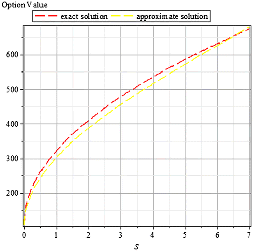
For numerical illustration, we will consider some examples for different values of S, t, and α over fixed values for the other parameters. Hence, for r = 0.06, |ρ| = 0.01, σ = 0.4, and S₀ = 4, we thus have the exact solution and initial condition as:(4.14) $$w\left(S,t\right)=S+200\left(\sqrt{S}exp\left(\frac{t}{20}\right)+\frac{1}{2}exp\left(\frac{t}{10}\right)\right),$$(4.14) (4.15) $$w\left(S,0\right)=S+200\sqrt{S}+100.$$(4.15)

Thus, by applying the MDTM with the above parameters, we get the following:(4.16) $$W_{S,0}=100+200\sqrt{S}+S,$$(4.16) (4.17) $$W_{S,1}=\frac{1}{1250\mathrm{\Gamma }\left(1+\mathit{\alpha }\right)}\left(5000-2500S^{1/2}-75S+600S^2+1200S^{5/2}+6S^3\right),$$(4.17) (4.18) $$W_{S,2}=\frac{1}{312500\mathrm{\Gamma }\left(1+2\mathit{\alpha }\right)}\left(\begin{array}{c}-125000+31250S^{1/2}+5625S-240000S^{3/2}\hfill \\ -1080000S^2-697200S^{5/2}-5400S^3\hfill \\ +3600S^4+7200S^{9/2}+36S^5\hfill \end{array}\right),⋮$$(4.18)

Whence,(4.19) $$w\left(S,t\right)=\sum _{h=0}^{\infty }{W}_{S,h}{t}^{h\mathit{\alpha }}=W_{S,0}+W_{S,1}{t}^{\mathit{\alpha }}+W_{S,2}{t}^{2\mathit{\alpha }}+W_{S,3}{t}^{3\mathit{\alpha }}+\cdots =\left(100+200\sqrt{S}+S\right)+\left(\frac{1}{2500\mathrm{\Gamma }\left(1+\mathit{\alpha }\right)}\left(5000-2500S^{1/2}-75S+600S^2+1200S^{5/2}+6S^3\right)\right)t^{\mathit{\alpha }}+\left\{\frac{1}{312500\mathrm{\Gamma }\left(1+2\mathit{\alpha }\right)}\left(-125000+31250S^{1/2}+5625S-240000S^{3/2}\right.\right.\left.\left.-1080000S^2-697200S^{5/2}-5400S^3+3600S^4+7200S^{9/2}+36S^5\right)\right\}{t}^{2\mathit{\alpha }}+\cdots .$$(4.19)

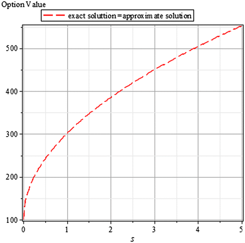
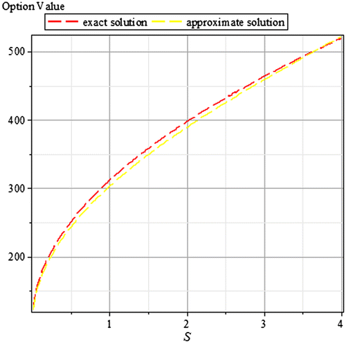
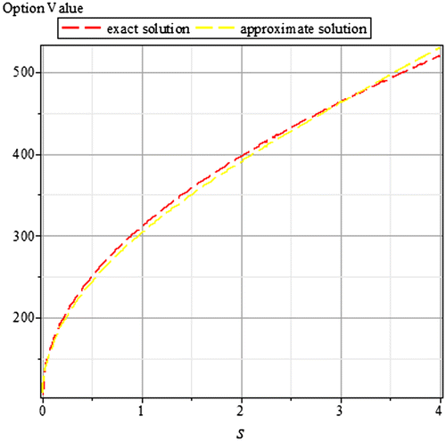
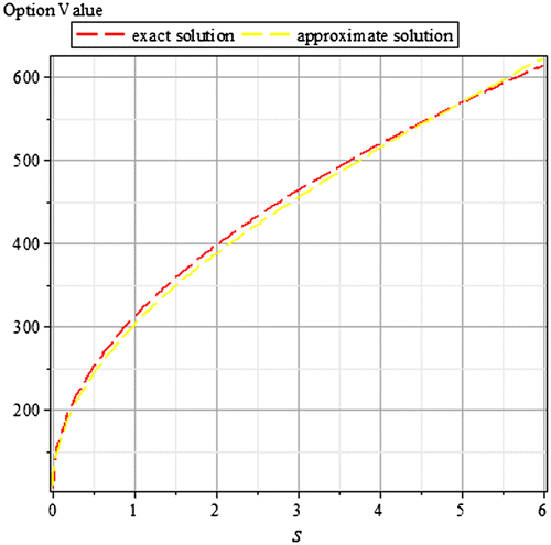
Tables 1 and 2 are for case 1 for an integer power of the time parameter, the graphs of same are in Figures 1 and 2, respectively. In a similar way, Tables 3^{Table 4}–5 are for case 2 for fractional powers of the time parameter, the graphs of same are in Figures 3^{Figure 4}–5, respectively. Also, we present in comparison the exact and the approximate solutions for different values of t and α, with $\left|{\sout{w}}_r\right|=\left|\left(w_{\text{exact}}-w_{\text{approx}}\right)/w_{\text{exact}}\right|$ as the relative error.

Table 1. Case 1 for t = 0 and α = 1

S	wexact	wapprox	$\left|{\sout{w}}_{\text{r}}\right|$
0.5	241.9214	241.9214	0.0000
1.0	301.0000	301.0000	0.0000
1.5	346.4490	346.4490	0.0000
2.0	384.8428	384.8428	0.0000
2.5	418.7278	418.7278	0.0000
3.0	449.4102	449.4102	0.0000
3.5	477.6658	477.6658	0.0000
4.0	504.0000	504.0000	0.0000
4.5	528.7641	528.7641	0.0000
5.0	552.2136	552.2136	0.0000

Table 2. Case 1 for t = 0.5 and  α = 1

S	wexact	wapprox	$\left|{\sout{w}}_{\text{r}}\right|$
0.5	250.6286	243.2212	0.029555
1.0	311.1902	301.9564	0.029673
1.5	357.777	347.1821	0.029613
2.0	397.1301	385.4947	0.029299
2.5	431.8603	419.4882	0.028648
3.0	463.3067	450.5316	0.027574
3.5	492.2649	479.4798	0.025972
4.0	519.2532	506.934	0.023725
4.5	544.6315	533.3594	0.020697

Figure 1. Graph for case 1 w.r.t. Table 1.

Figure 2. Graph for case 1 w.r.t. Table 2.

Table 3. Case 2 for t = 0.5 and α = 0.5

S	wexact	wapprox	$\left|{\sout{w}}_{\text{r}}\right|$
0.01	125.6435	123.2255	0.019245
0.02	134.1475	131.455	0.020071
0.03	140.6751	137.7714	0.020641
0.04	146.1798	143.0975	0.021086
0.05	151.0306	147.7904	0.021454
0.06	155.4171	152.0336	0.021770
0.07	159.4517	155.9358	0.022050
0.08	163.2077	159.5681	0.022300
0.09	166.7361	162.9796	0.022530
0.10	170.0738	166.2063	0.022740

Table 4. Case 2 for t = 0.5 and α = 1.5

S	wexact	wapprox	$\left|{\sout{w}}_{\text{r}}\right|$
0.01	125.6435	121.0283	0.036733
0.02	134.1475	129.3005	0.036132
0.03	140.6751	135.6503	0.035719
0.04	146.1798	141.005	0.035400
0.05	151.0306	145.7237	0.035138
0.06	155.4171	149.9908	0.034914
0.07	159.4517	153.9156	0.034720
0.08	163.2077	157.5695	0.034546
0.09	166.7361	161.0019	0.034391
0.10	170.0738	166.2063	0.022740

Table 5. Case 2 for t = 1 and α = 2.5

S	wexact	wapprox	$\left|{\sout{w}}_{\text{r}}\right|$
0.01	131.5526	121.1564	0.079027
0.02	140.2716	129.4256	0.077321
0.03	146.9642	135.7732	0.076148
0.04	152.608	141.126	0.075239
0.05	157.5814	145.8432	0.074490
0.06	162.0787	150.1088	0.073852
0.07	166.2152	154.0323	0.073296
0.08	170.066	157.6850	0.072801
0.09	173.6834	161.1163	0.072356
0.10	177.1054	164.3623	0.071952

Figure 3. Graph for case 2 w.r.t. Table 3.

Figure 4. Graph for case 2 w.r.t. Table 4.

Figure 5. Graph for case 2 w.r.t. Table 5.

5. Concluding remarks

In this paper, we considered analytical solutions of a time-fractional nonlinear transaction-cost model for stock option valuation in an illiquid market setting driven by a relaxed Black–Scholes model assumption through a relatively new semi-analytical method called the modified differential transform method (MDTM). Firstly, we considered a nonlinear option pricing model obtained when the constant volatility assumption of the famous linear Black–Scholes option pricing model is relaxed through the inclusion of transaction cost. Thereafter, we extend, for the first time in literature, this nonlinear option pricing model to a time-fractional ordered form, and obtained approximate-analytical solutions to this new nonlinear model via the proposed solution technique. For efficiency and reliability of the method, we considered two cases with five examples: case 1 with two examples for time-integer order, and case 2 with three examples for time-fractional order. Our results are very interesting, they conform with the associated exact solutions obtained by Esekon (2013), and those of González-Gaxiola et al. (2015) using the Adomian decomposition method; even though our approximate solutions include only terms up to time power three (3), accuracy is improved for more terms. This therefore shows that the work of González-Gaxiola et al. (2015) is a particular case of our present work when α = 1. Maple 18 software is used for all the numerical computations done in this work. Hence, the method is a good candidate for solving linear and nonlinear differential equations (models) with time- or space fractional orders, though the application of the method to differential equations (linear and nonlinear option pricing models) with complex-fractional orders is yet to be considered in its wider sense.

Funding

This work was supported by Covenant University [grant number CUCRID/PSG/VC/17/07/14-FS].

Acknowledgements

The authors are sincerely grateful to Covenant University for financial support and provision of good working environment. They also wish to thank the anonymous referee(s) for their constructive and helpful comments.

Additional information

Notes on contributors

S.O. Edeki

S.O. Edeki is a lecturer at the Department of Mathematics, Covenant University, Ota, Nigeria. His research areas include financial mathematics, fractional calculus, and stochastic differential equations. He has published reasonable number of research articles in reputable international journals indexed and abstracted in scopus/ISI.

O.O. Ugbebor

O.O. Ugbebor serves as a full professor at the Department of Mathematics, University of Ibadan, Nigeria. She received her BSc and PhD degrees from University of Ibadan, Nigeria and University of London, respectively. Her research areas include probability theory, stochastic processes, and financial mathematics. She has good number of published articles in well-indexed journals both at local and international levels.

E.A. Owoloko

E.A. Owoloko is a senior lecturer at the Department of Mathematics, Covenant University, Ota, Nigeria. He obtained his PhD degree from Covenant University. His research areas include financial mathematics and operation research. He has many research papers in well-indexed journals.

References

- Acharya, V., & Pedersen, L. H. (2005). Asset pricing with liquidity risk. Journal of Financial Economics, 77, 375–410.10.1016/j.jfineco.2004.06.007
- Ahmad, J., Shakeel, M., Hassan, Q. M. U. I., & Mohyud-Din, S. T. (2013). Analytical solution of Black–Scholes model using fractional variational iteration method. International Journal of Modern Mathematical Sciences, 5, 133–142.
- Allahviranloo, T., & Behzadi, Sh. S. (2013). The use of iterative methods for solving Black–Scholes equation. International Journal of Industrial Mathematics, 5(1), 1–11, Article ID IJIM-00329.
- Amihud, Y., & Mendelson, H. (1986). Asset pricing and the bid-ask spread. Journal of Financial Economics, 17, 223–249.10.1016/0304-405X(86)90065-6
- Ankudinova, J., & Ehrhardt, M. (2008). On the numerical solution of nonlinear Black–Scholes equations. Computers & Mathematics with Applications, 56, 799–812.10.1016/j.camwa.2008.02.005
- Bakstein, D., & Howison, S. (2003). A non-arbitrage liquidity model with observable parameters for derivatives. Oxford: Oxford University Preprint.
- Barles, G., & Soner, H. M. (1998). Option pricing with transaction costs and a nonlinear Black–Scholes equation. Finance and Stochastics, 2, 369–397.10.1007/s007800050046
- Black, F., & Scholes, M. (1973). The pricing options and corporate liabilities. Journal of Political Economy, 81, 637–654.10.1086/260062
- Bohner, M., & Zheng, Y. (2009). On analytical solutions of the Black–Scholes equation. Applied Mathematics Letters, 22, 309–313.10.1016/j.aml.2008.04.002
- Boyle, P., & Vorst, T. (1992). Option replication in discrete time with transaction costs. The Journal of Finance, 47, 271–293.10.1111/j.1540-6261.1992.tb03986.x
- Cen, Z., & Le, A. (2011). A robust and accurate finite difference method for a generalized Black–Scholes equation. Journal of Computational and Applied Mathematics, 235, 3728–3733.10.1016/j.cam.2011.01.018
- Cetin, U., Jarrow, R. A., & Protter, P. (2004). Liquidity risk and arbitrage pricing theory. Finance Stochast, 8, 311–341. doi:10.1007/s00780-003-0123-2
- Company, R., Navarro, E., Ramón Pintos, J. R., & Ponsoda, E. (2008). Numerical solution of linear and nonlinear Black–Scholes option pricing equations. Computers & Mathematics with Applications, 56, 813–821.10.1016/j.camwa.2008.02.010
- Edeki, S. O., Akinlabi, G. O., & Adeosun, S. A. (2016a). Analytic and numerical solutions of time-fractional linear Schrödinger equation. Communications in Mathematics and Applications, 7(1), 1–10.
- Edeki, S. O., Akinlabi, G. O., & Adeosun, S. A. (2016b). On a modified transformation method for exact and approximate solutions of linear Schrödinger equations. AIP Conference Proceedings, 1705, 020048. doi:10.1063/1.4940296
- Edeki, S. O., Owoloko, E. A., & Ugbebor, O. O. (2016). The modified Black–Scholes model via constant elasticity of variance for stock options valuation. AIP Conference proceedings, 1705, 020041. doi:10.1063/1.4940289
- Edeki, S. O., & Ugbebor, O. O. (2015, 23–26 June). A remark on the solution of Black–Scholes model for theoretical values of European options. In 34th Annual Conference of the Nigerian Mathematical Society. Lagos: University of Lagos.
- Edeki, S. O., Ugbebor, O. O., & Owoloko, E. A. (2015). Analytical solutions of the Black–Scholes pricing model for european option valuation via a projected differential transformation method. Entropy, 17, 7510–7521.10.3390/e17117510
- Edeki, S. O., Ugbebor, O. O., & Owoloko, E. A. (2016). A note on Black–Scholes pricing model for theoretical values of stock options. AIP Conference Proceedings, 1705, 020040. doi:10.1063/1.4940288
- Elbeleze, A. A., Kilicman, A., & Taib, B. M. (2013). Homotopy perturbation method for fractional Black–Scholes European option pricing equations using Sumudu transform. Mathematical Problems in Engineering, 1–7.
- Esekon, J. E. (2013). Analytic solution of a nonlinear Black–Scholes equation. International Journal of Pure and Applied Mathematical Sciences, 82, 547–555.
- Frey, R., & Patie, P. (2002). Risk management for derivatives in illiquid markets: A simulation study. In K. Sandmann & P. J. Schönbucher (Eds.), Advances in finance and stochastics (pp. 137–159). Berlin: Springer.10.1007/978-3-662-04790-3
- Frey, R., & Stremme, A. (1997). Market volatility and feedback effects from dynamic hedging. Mathematical Finance, 7, 351–374.10.1111/mafi.1997.7.issue-4
- Ghandehari, M. A. M., & Ranjbar, M. (2014). European option pricing of fractional version of the Black–Scholes model: Approach via expansion in series. International Journal of Nonlinear Science, 17, 105–110.
- González-Gaxiola, O., Ruíz de Chávez, J., & Santiago, J. A. (2015). A nonlinear option pricing model through the adomian decomposition method. International Journal of Applied and Computational Mathematics, 1(2), 1–15.
- Hariharan, G. (2013). An efficient wavelet based approximation method to time fractional Black–Scholes European option pricing problem arising in financial market. Applied Mathematical Sciences, 7, 3445–3456.10.12988/ams.2013.35261
- He, J. H. (1999). Some applications of nonlinear fractional differential equations and their approximations. Science, Technology and Society, 15, 86–90.
- Ibis, B., Bayram, M., & Agargun, A. G. (2011). Applications of fractional differential transform method to fractional differential-algebraic equations. European Journal of Pure and Applied Mathematics, 4, 129–141.
- Jang, B. (2010). Solving linear and nonlinear initial value problems by the projected differential transform method. Computer Physics Communications, 181, 848–854.10.1016/j.cpc.2009.12.020
- Jódar, L., Sevilla-Peris, P., Cortés, J. C., & Sala, R. (2005). A new direct method for solving the Black–Scholes equation. Applied Mathematics Letters, 18, 29–32.10.1016/j.aml.2002.12.016
- Keskin, Y., Servi, S., & Oturanç, G. (2011, July 6–8). Reduced differential transform method for solving Klein Gordon equations. In Proceedings of the World Congress on Engineering (WCE). London.
- Keynes, J. M. (1971). A treatise on money: The pure theory of money. (E. Johnson and D. Moggridge Eds.). London: Macmillan.
- Khan, W. A., & Ansari, F. A. (2016). European option pricing of fractional Black–Scholes model using Sumudu transform and its derivatives. General Letters in Mathematcis, 1, 64–74.
- Kilbas, A. A., Srivastava, H. M., & Trujilo, J. J. (2006). Theory and applications of fractional differential equations. North-Holland Mathematical Studies, 204.
- Kumar, S., Yildirin, A., Khan, Y., Jafari, H., Sayevand, K., & Wei, L. (2012). Analytical solution of fractional Black–Scholes European option pricing equations using Laplace transform. Journal of Fractional Calculus and Applications, 2(8), 1–9.
- Kumar, S., Kumar, D., & Singh, J. (2014). Numerical computation of fractional Black–Scholes equation arising in financial market. Egyptian Journal of Basic and Applied Sciences, 1, 177–183.10.1016/j.ejbas.2014.10.003
- Liu, H., & Yong, J. (2005). Option pricing with an illiquid underlying asset market. Journal of Economic Dynamics and Control, 29, 2125–2156.10.1016/j.jedc.2004.11.004
- Miller, K. S., & Ross, B. (1993). An introduction to the fractional calculus and fractional differential equations. New York, NY: John Wiley & Sons.
- Mokhtary, P., Ghoreishi, F., & Srivastava, H. M. (2016). The Müntz–Legendre Tau method for fractional differential equations. Applied Mathematical Modelling, 40, 671–684.10.1016/j.apm.2015.06.014
- Podlubny, I. (1999). Fractional differential equations. San Diego, CA: Academic Press.
- Ravi Kanth, A. S. V., & Aruna, K. (2012). Comparison of two dimensional DTM and PTDM for solving time-dependent Emden–Fowler type equations. International Journal of Nonlinear Science, 13, 228–239.
- Ravi Kanth, A. S. V., & Aruna, K. (2016). ,Solution of time fractional Black–Scholes European option pricing equation arising in financial market. Nonlinear Engineering, 5, 269–276. doi:10.1515/nleng-2016-0052
- Rodrigo, M. R., & Mamon, R. S. (2006). An alternative approach to solving the Black–Scholes equation with time-varying parameters. Applied Mathematics Letters, 19, 398–402.10.1016/j.aml.2005.06.012
- Song, J., Yin, F., Cao, X., & Lu, F. (2013). Fractional variational iteration method versus Adomian’s decomposition method in some fractional partial differential equations. Journal of Applied Mathematics, Article ID 392567, 10.