The improved F-expansion method and its application to the MEE circular rod equation and the ZKBBM equation

Abstract

In the present article, we implement the improved F-expansion method combined with Riccati equation to attain traveling wave solutions to nonlinear evolution equations (NLEEs) via the Magneto-electro-elastic circular rod equation and the Zakharov-Kuznetsov-Benjamin-Bona-Mahony equation. We establish three classes of explicit solutions-hyperbolic, trigonometric and rational solutions containing several free parameters. For particular values of the parameters, solitary wave solutions are emanated from the traveling wave solutions. It turns out that, the method is straightforward, concise and it can be applied to many other NLEEs in mathematical physics and engineering.

Keywords:

• improved F-expansion method
• MEE circular rod equation
• ZKBBM equation
• exact solution
• traveling wave
• NLEEs

Mathematics Subject Classifications:

• 35C07
• 35C08
• 35K99
• 35P05
• 35P99

Public Interest Statement

As we know, nonlinear evolution equations (NLEEs) are largely used to designate complex phenomena in numerous fields of science, such as plasma physics, solid state physical and optical fibers, chemical kinematics, chemical physics, and geochemistry. So it is important to develop various methods for solving different NLEEs. In this present article, we use the improved F-expansion method combined with Riccati equation for seeking abundant exact traveling wave solutions to the Magneto-electro-elastic (MEE) circular rod equation and the Zakharov-Kuznetsov-Benjamin-Bona-Mahony (ZKBBM) equation. The current method is effective, simple, and suitable that can be extended to solve the system of NLEEs arising in mathematical physics and Engineering fields. The obtained exact solutions might play a crucial role to expose the inner composition of the physical phenomena.

1. Introduction

Nowadays in the field of nonlinear science, the study of the traveling wave solutions of NLEEs plays a significant role in several features of mathematical and physical phenomena. Nonlinear wave phenomena appears in various scientific and engineering fields such as optical fibers, biology, solid state physics, chemical kinematics, meteorology, chemical physics, and geochemistry. Nonlinear wave phenomena of dispersion, dissipation, diffusion, feedback and convection are very noteworthy in nonlinear wave equations. The search to exact traveling wave solutions of NLEEs has been one of the most attractive and dynamic area of research to the mathematics, mathematical physicists, and engineers. With the improvement of symbolic computation software like Maple and Mathematica, many powerful and effective methods to find analytical and numerical solutions of nonlinear equations still have drawn a lot of attention by diverse group of investigators.

The exact solutions of NLEEs support us by providing information about the structure of intricate physical phenomena. Therefore, investigation of exact traveling wave solutions to NLEEs turns into an important task in the study of nonlinear physical phenomena. It is notable to observe that there is no unique method to solve all kind of NLEEs. There are lots of nonlinear evolution equations that are investigated by using different mathematical methods. For these physical problems, soliton solutions, compacton, cnoidal waves, singular solitons, and the other solutions have been found. These types of solutions appear in various applications of applied science and engineering. In order to find the exact solutions, especially the traveling wave solutions of the NLEEs, various powerful methods are reported in the literature, such as, the Hirota’s bilinear method (Ashorman, 2014), the truncated Painleve expansion method (Yin-Long, Yin-Ping, & Zhi-Bin, 2010), the Exp-function method (Akbar & Ali, 2011; Zhang, 2008a, 2008b), the tanh-function method (Abdou, 2007; Zayed, Zedan, & Gepreel, 2004; Zhang & Xia, 2008), the Weierstrass elliptic function method (Chen & Yan, 2006), the Jacobi elliptic function expansion method (Chen & Wang, 2005; Wazwaz, 2008; Yusufoglu & Bekir, 2008), the modified simple equation method (Jawad, Petkovic, & Biswas, 2010; Khan & Akbar, 2013a, 2014), the (G′/G)-expansion method (Guo & Zhou, 2010; Islam, Khan, & Akbar, 2015; Kim & Sakthivel, 2012; Wang, Li, & Zhang, 2008; Zayed & Gepreel, 2009), the exp (Φ(ξ))-expansion method (Khan & Akbar, 2013b), the improved F-expansion method (Islam, Khan, Akbar, & Mastroberardino, 2014; Zgang, Wang, Wang, & Fang, 2006), the modified method of simplest equation (Vitanov & Dimitrova, 2014), the F-expansion method (Zhao, 2013), and the generalized Kudryashov method (Islam, Khan, & Akbar, 2015, 2015b).

The objective of this article is to look for new study concerning to the improved F-expansion method combined with Riccati equation to scrutinize exact traveling wave solutions to the MEE circular rod equation and the ZKBBM equation to establish the efficiency and advantages of the method. The MEE circular rod equation is a nonlinear traveling wave equation with dispersion caused by the transverse Poisson’s effect. The ZKBBM equation was studied as an improvement of the KdV equation for modeling long surface gravity waves of small amplitude propagating uni-directionally in (1+1)-dimensions. The solutions of this equation are stable and unique. The exact solutions play a fundamental role to expose the inner composition of the physical phenomena.

The rest of the article is arranged as follows: in the Section 2, the improved F-expansion method is sketched. In Section 3, we apply this method to extract new exact solutions via the MEE circular rod equation and the ZKBBM equation. Advantages of the method are discussed in Section 4. In Section 5, the explanation and graphical representations of certain attained solutions are provided. Finally, in the Section 6, conclusions of this study are given.

2. Delineation of the improved F-expansion method

In this section, we describe the fundamental steps of the improved F-expansion method to obtain the exact solutions of NLEEs. At the outset, we consider the celebrated Riccati equation of the form:(2.1) $$F^{\prime }(\mathit{\eta })=r+F^2(\mathit{\eta }),$$(2.1)

where the prime stands for derivative with respect to η.

We now present three cases of the general solutions of the Riccati Equation (2.1) (Cruz, Schuch, Castanos, & Rosas-Ortiz, 2015).

Case-I: When r < 0, the general solutions are$$\begin{array}{c}{F}_1=-\sqrt{-r}tanh\left(\sqrt{-r}\mathit{\eta }\right),\hfill \\ F_2=-\sqrt{-r}coth\left(\sqrt{-r}\mathit{\eta }\right),\hfill \end{array}$$

Case-II: When r > 0, the general solutions are$$\begin{array}{c}{F}_3=\sqrt{r}tan\left(\sqrt{r}\mathit{\eta }\right),\hfill \\ F_4=-\sqrt{r}cot\left(\sqrt{r}\mathit{\eta }\right),\hfill \end{array}$$

Case-III: When r = 0, the general solution is$$F_5=-\frac{1}{\mathit{\eta }}.$$

We consider a general NLEE in two independent variables, say x and t,(2.2) $$\mathrm{\Phi }(u,u_x,u_t,u_{xx},u_{xt},\cdots )=0,$$(2.2)

where $u=u(x,t)$ is an unknown function to be determined, Φ is a polynomial of $u(x,t)$ and its partial derivatives wherein the highest order partial derivatives and the nonlinear terms are involved and the subscripts indicate the partial derivatives. The key steps of the method are as follows:

Step-1: We now introduce the traveling wave variable,(2.3) $$\mathit{\eta }=x\pm \mathit{\omega }t,u(x,t)=u(\mathit{\eta }),$$(2.3)

where ω is the speed of traveling wave and the wave variable (2.3) transforms Equation (2.2) into the following ordinary differential equation (ODE):(2.4) $$\mathrm{\Theta }(u,u^{\prime },u^{″},u^{\prime ″},\cdots )=0,$$(2.4)

where Θ is a polynomial of u and its derivatives and the superscripts stipulate the ordinary derivatives with respect to η.

Step-2: In many instances, Equation (2.4) can be integrated term by term one or more times, yielding constants of integration, which can be set equal to zero for straightforwardness.

Step-3: We assume that the traveling wave solution of Equation (2.4) can be expressed by a polynomial in $F(\mathit{\eta })$ as follows:(2.5) $$u(\mathit{\eta })=\sum _{i=0}^N{\mathit{\alpha }}_i{\left(\mathit{\mu }+F(\mathit{\eta })\right)}^i+\sum _{i=1}^N{\mathit{\beta }}_i{\left(\mathit{\mu }+F(\mathit{\eta })\right)}^{-i},$$(2.5)

where $F=F(\mathit{\eta })$ satisfies the Riccati Equation (2.1), wherein either α_N or β_N may be zero, but both of them could not be zero at the same time. ${\mathit{\alpha }}_i(i=0,1,2,\cdots ,N)$ and ${\mathit{\beta }}_i(i=0,1,2,\cdots ,N)$, ω and μ are arbitrary constants to be determined later.

Step-4: The positive integer N can be determined by using the homogeneous balance between the highest order derivatives and the nonlinear terms appearing in (2.4). If the degree of u(η) is D[u(η)] = N, then the degree of the other expressions can be computed as follows:(2.6) $$D\left[\frac{d^{p}u(\mathit{\eta })}{d{\mathit{\eta }}^p}\right]=N+p,D\left[u^p{\left(\frac{d^{q}u(\mathit{\eta })}{d{\mathit{\eta }}^q}\right)}^s\right]=Np+s\left(N+p\right).$$(2.6)

Therefore, we can find the value of N appearing in (2.5) by using (2.6).

Step-5: Substituting (2.5) into (2.4) together with the value of N attained in Step 4, we reach a polynomial in $F(\mathit{\eta })$. We set each coefficient of the resulting polynomial to zero, yield an over-determined set of algebraic equations for α_i, β_i, μ, and ω.

Step-6: We stare that the value of the constants α_i, β_i, μ, and ω can be determined by solving the algebraic equations achieved in Step 5. Since the general solution of (2.1) is in general known, inserting the value of α_i, β_i, μ, and ω into (2.5) yields the comprehensive and newly produced exact traveling wave solutions of the nonlinear partial differential Equation (2.2). This completes the determination of the exact traveling wave solutions.

3. Applications

In this section, we make use of the improved F-expansion method to obtain some new and more general exact traveling wave solutions of the MEE circular rod equation and the ZKBBM equation.

3.1. Magneto-electro-elastic (MEE) circular rod equation

Let us consider the Magneto-electro-elastic (MEE) circular rod equation (Xue & Pan, 2013) in the form(3.1.1) $$u_{tt}-c_0^2{u}_{xx}-{\left(\frac{c_0^2}{2}{u}^2+N{u}_{tt}\right)}_{xx}=0,$$(3.1.1)

where c₀ is the linear longitudinal wave velocity for a MEE circular rod equation and N is the dispersion parameter, both depend on the material properties as well as the geometry of the rod. Equation (3.1.1) is a nonlinear traveling wave equation with dispersion caused by the transverse Poisson’s effect. We consider the traveling wave transformation equation(3.1.2) $$\mathit{\eta }=r(x-\mathit{\omega }t),u(x,t)=u(\mathit{\eta }),$$(3.1.2)

which reduces Equation (3.1.1) into the following ODE:(3.1.3) $$r^2{\mathit{\omega }}^2{u}^{″}-r^2{c}_0^2{u}^{″}-r^2{\left(\frac{c_0^2}{2}{u}^2+N{r}^2{\mathit{\omega }}^2{u}^{″}\right)}^{″}=0,$$(3.1.3)

Equation (3.1.3) is integrable. Integrating Equation (3.1.3) twice with respect to η, and setting the constants of integration to zero, we obtain(3.1.4) $$\left({\mathit{\omega }}^2-c_0^2\right)u-\frac{c_0^2}{2}{u}^2-N{r}^2{\mathit{\omega }}^2{u}^{″}=0,$$(3.1.4)

Balancing the highest order nonlinear term u² and the derivative term u^″, Equation (3.1.4) yields N = 2.

Hence, for N = 2, solution Equation (2.5) reduces to(3.1.5) $$u(\mathit{\eta })={\mathit{\alpha }}_0+{\mathit{\alpha }}_1\left(\mathit{\mu }+F(\mathit{\eta })\right)+{\mathit{\alpha }}_2{\left(\mathit{\mu }+F(\mathit{\eta })\right)}^2+{\mathit{\beta }}_1{\left(\mathit{\mu }+F(\mathit{\eta })\right)}^{-1}+{\mathit{\beta }}_2{\left(\mathit{\mu }+F(\mathit{\eta })\right)}^{-2},$$(3.1.5)

where ${\mathit{\alpha }}_0,{\mathit{\alpha }}_1,{\mathit{\alpha }}_2,{\mathit{\beta }}_1$ and β₂ are arbitrary constant to be determined later. Now substituting (3.1.5) into (3.1.4), we obtain a polynomial in $F(\mathit{\eta })$. Equating the coefficient of same power $F(\mathit{\eta })$, we acquire a system of twelve algebraic equations. Solving this system of equations for ${\mathit{\alpha }}_0,{\mathit{\alpha }}_1,{\mathit{\alpha }}_2,{\mathit{\beta }}_1,{\mathit{\beta }}_2$ and ω, we obtain the following values:$$\text{Set-}01:\begin{array}{c}\mathit{\omega }=\pm \frac{c_0}{\sqrt{4N{r}^3+1}},{\mathit{\alpha }}_0=-\frac{12N{r}^2\left({\mathit{\mu }}^2+r\right)}{4N{r}^3+1},{\mathit{\alpha }}_1=\frac{24N{r}^2\mathit{\mu }}{4N{r}^3+1},{\mathit{\alpha }}_2=-\frac{12N{r}^2}{4N{r}^3+1},\hfill \\ {\mathit{\beta }}_1=0,{\mathit{\beta }}_2=0.\hfill \end{array}$$$$\text{Set-}02:\begin{array}{c}\mathit{\omega }=\pm \frac{c_0}{\sqrt{1-4N{r}^3}},{\mathit{\alpha }}_0=\frac{4N{r}^2\left(3{\mathit{\mu }}^2+r\right)}{4N{r}^3-1},{\mathit{\alpha }}_1=-\frac{24N{r}^2\mathit{\mu }}{4N{r}^3-1},{\mathit{\alpha }}_2=\frac{12N{r}^2}{4N{r}^3-1},\hfill \\ {\mathit{\beta }}_1=0,{\mathit{\beta }}_2=0.\hfill \end{array}$$$$\text{Set-}03:\begin{array}{c}\mathit{\omega }=\pm \frac{c_0}{\sqrt{4N{r}^3+1}},{\mathit{\alpha }}_0=-\frac{12N{r}^2\left({\mathit{\mu }}^2+r\right)}{4N{r}^3+1},{\mathit{\alpha }}_1=0,{\mathit{\alpha }}_2=0,\hfill \\ {\mathit{\beta }}_1=\frac{24N{r}^2\mathit{\mu }({\mathit{\mu }}^2+r)}{4N{r}^3+1},{\mathit{\beta }}_2=-\frac{12N{r}^2{\left({\mathit{\mu }}^2+4\right)}^2}{4N{r}^3+1}.\hfill \end{array}$$$$\text{Set-}04:\begin{array}{c}\mathit{\omega }=\pm \frac{c_0}{\sqrt{1-4N{r}^3}},{\mathit{\alpha }}_0=\frac{4N{r}^2\left(3{\mathit{\mu }}^2+r\right)}{4N{r}^3-1},{\mathit{\alpha }}_1=0,{\mathit{\alpha }}_2=0,\hfill \\ {\mathit{\beta }}_1=-\frac{24N{r}^2\mathit{\mu }({\mathit{\mu }}^2+r)}{4N{r}^3-1},{\mathit{\beta }}_2=\frac{12N{r}^2{\left({\mathit{\mu }}^2+4\right)}^2}{4N{r}^3-1}.\hfill \end{array}$$

The above sets of values of ${\mathit{\alpha }}_0,{\mathit{\alpha }}_1,{\mathit{\alpha }}_2,{\mathit{\beta }}_1,{\mathit{\beta }}_2$ and ω provides the subsequent abundant exact traveling wave solutions:

Case-I: When r < 0, we get the following hyperbolic function solutions.(3.1.6) $$\text{Family-}01:u_1\left(\mathit{\eta }\right)=-\frac{12N{r}^3}{4N{r}^3+1}sec{h}^2\left(\sqrt{-r}\mathit{\eta }\right),$$(3.1.6) (3.1.7) $$u_2(\mathit{\eta })=\frac{12N{r}^3}{4N{r}^3+1}csc{h}^2\left(\sqrt{-r}\mathit{\eta }\right),$$(3.1.7)

where $\mathit{\eta }=r\left(x-\frac{c_0}{\sqrt{4N{r}^3+1}}t\right)$.(3.1.8) $$\text{Family-}02:u_3\left(\mathit{\eta }\right)=\frac{4N{r}^3}{4N{r}^3-1}\left(1-3{tanh}^2\left(\sqrt{-r}\mathit{\eta }\right)\right),$$(3.1.8) (3.1.9) $$u_4(\mathit{\eta })=\frac{4N{r}^3}{4N{r}^3-1}\left(1-3{coth}^2\left(\sqrt{-r}\mathit{\eta }\right)\right),$$(3.1.9)

where $\mathit{\eta }=r\left(x-\frac{c_0}{\sqrt{1-4N{r}^3}}t\right)$.(3.1.10) $$\text{Family-}03:u_5\left(\mathit{\eta }\right)=-\frac{12N{r}^3\left({\mathit{\mu }}^2+r\right)}{\left(4N{r}^3+1\right){\left(-\mathit{\mu }+\sqrt{-r}tanh\left(\sqrt{-r}\mathit{\eta }\right)\right)}^2}sec{h}^2\left(\sqrt{-r}\mathit{\eta }\right),$$(3.1.10) (3.1.11) $$u_6(\mathit{\eta })=-\frac{12N{r}^3\left({\mathit{\mu }}^2+r\right)}{\left(4N{r}^3+1\right){\left(-\mathit{\mu }+\sqrt{-r}tanh\left(\sqrt{-r}\mathit{\eta }\right)\right)}^2}csc{h}^2\left(\sqrt{-r}\mathit{\eta }\right),$$(3.1.11)

where $\mathit{\eta }=r\left(x-\frac{c_0}{\sqrt{4N{r}^3+1}}t\right)$.(3.1.12) $$\text{Family-}04:u_7\left(\mathit{\eta }\right)=\frac{4N{r}^3\left(\begin{array}{c}\hfill {\mathit{\mu }}^2-3{\mathit{\mu }}^2{tanh}^2\left(\sqrt{-r}\mathit{\eta }\right)+4\mathit{\mu }\sqrt{-r}tanh\left(\sqrt{-r}\mathit{\eta }\right)\\ \hfill -r{tanh}^2\left(\sqrt{-r}\mathit{\eta }\right)+3r\\ \hfill \end{array}\right)}{\left(4N{r}^3-1\right){\left(-\mathit{\mu }+\sqrt{-r}tanh\left(\sqrt{-r}\mathit{\eta }\right)\right)}^2},$$(3.1.12) (3.1.13) $$u_8(\mathit{\eta })=\frac{4N{r}^3\left(\begin{array}{c}{\mathit{\mu }}^2-3{\mathit{\mu }}^2{coth}^2\left(\sqrt{-r}\mathit{\eta }\right)+4\mathit{\mu }\sqrt{-r}coth\left(\sqrt{-r}\mathit{\eta }\right)\\ -r{coth}^2\left(\sqrt{-r}\mathit{\eta }\right)+3r\\ \end{array}\right)}{\left(4N{r}^3-1\right){\left(-\mathit{\mu }+\sqrt{-r}coth\left(\sqrt{-r}\mathit{\eta }\right)\right)}^2},$$(3.1.13)

where $\mathit{\eta }=r\left(x-\frac{c_0}{\sqrt{1-4N{r}^3}}t\right)$.

Case-II: When r > 0, we get the following trigonometric solutions:(3.1.14) $$\text{Family-}05:u_9\left(\mathit{\eta }\right)=-\frac{12N{r}^3}{4N{r}^3+1}{sec}^2\left(\sqrt{r}\mathit{\eta }\right),$$(3.1.14) (3.1.15) $$u_{10}(\mathit{\eta })=-\frac{12N{r}^3}{4N{r}^3+1}{csc}^2\left(\sqrt{r}\mathit{\eta }\right),$$(3.1.15)

where $\mathit{\eta }=r\left(x-\frac{c_0}{\sqrt{4N{r}^3+1}}t\right)$.(3.1.16) $$\text{Family-}06:u_{11}\left(\mathit{\eta }\right)=\frac{4N{r}^3}{4N{r}^3-1}\left(1+3{tan}^2\left(\sqrt{r}\mathit{\eta }\right)\right),$$(3.1.16) (3.1.17) $$u_{12}(\mathit{\eta })=\frac{4N{r}^3}{4N{r}^3-1}\left(1+3{cot}^2\left(\sqrt{r}\mathit{\eta }\right)\right),$$(3.1.17)

where $\mathit{\eta }=r\left(x-\frac{c_0}{\sqrt{1-4N{r}^3}}t\right)$.(3.1.18) $$\text{Family-}07:u_{13}\left(\mathit{\eta }\right)=-\frac{12N{r}^3\left({\mathit{\mu }}^2+r\right)}{\left(4N{r}^3+1\right){\left(\mathit{\mu }+\sqrt{r}tan\left(\sqrt{r}\mathit{\eta }\right)\right)}^2}{sec}^2\left(\sqrt{r}\mathit{\eta }\right),$$(3.1.18) (3.1.19) $$u_{14}(\mathit{\eta })=-\frac{12N{r}^3\left({\mathit{\mu }}^2+r\right)}{\left(4N{r}^3+1\right){\left(-\mathit{\mu }+\sqrt{r}coth\left(\sqrt{r}\mathit{\eta }\right)\right)}^2}{csc}^2\left(\sqrt{r}\mathit{\eta }\right),$$(3.1.19)

where $\mathit{\eta }=r\left(x-\frac{c_0}{\sqrt{4N{r}^3+1}}t\right)$.(3.1.20) $$\text{Family-}08:u_{15}\left(\mathit{\eta }\right)=\frac{4N{r}^3\left(\begin{array}{c}\hfill {\mathit{\mu }}^2+3{\mathit{\mu }}^2{tan}^2\left(\sqrt{r}\mathit{\eta }\right)-4\mathit{\mu }\sqrt{r}tan\left(\sqrt{r}\mathit{\eta }\right)\\ \hfill +r{tan}^2\left(\sqrt{r}\mathit{\eta }\right)+3r\\ \hfill \end{array}\right)}{\left(4N{r}^3-1\right){\left(\mathit{\mu }+\sqrt{r}tan\left(\sqrt{r}\mathit{\eta }\right)\right)}^2},$$(3.1.20) (3.1.21) $$u_{16}(\mathit{\eta })=\frac{4N{r}^3\left(\begin{array}{c}{\mathit{\mu }}^2+3{\mathit{\mu }}^2{cot}^2\left(\sqrt{r}\mathit{\eta }\right)+4\mathit{\mu }\sqrt{r}cot\left(\sqrt{r}\mathit{\eta }\right)\\ +r{cot}^2\left(\sqrt{r}\mathit{\eta }\right)+3r\\ \end{array}\right)}{\left(4N{r}^3-1\right){\left(-\mathit{\mu }+\sqrt{r}cot\left(\sqrt{r}\mathit{\eta }\right)\right)}^2},$$(3.1.21)

where $\mathit{\eta }=r\left(x-\frac{c_0}{\sqrt{1-4N{r}^3}}t\right)$.

Remark

All of these solutions have been verified with Maple software by substituting them into the original equations and found accurate.

3.2. The Zakharov-Kuznetsov-Benjamin-Bona-Mahony (ZKBBM) equation

In this subdivision, we construct the exact solutions of the ZKBBM equation by using the proposed method. This equation was studied as an improvement of the KdV equation for modeling long surface gravity waves of small amplitude propagating uni-directionally in (1+1)-dimensions. The solutions of this equation are stable and unique. This contrasts with the KdV equation, which is unstable in its high wave number components. We consider the ZKBBM equation (Akbar, Ali, & Zayed, 2012) in the form(3.2.1) $$u_t+u_x-2au{u}_x-b{u}_{xxt}=0,$$(3.2.1)

where a and b are positive constants. We substitute the traveling wave transformation $\mathit{\eta }=r(x-\mathit{\omega }t),u(x,t)=u(\mathit{\eta }),$ into (3.2.1) and obtain the ODE:(3.2.2) $$(1-\mathit{\omega })u^{\prime }-2au{u}^{\prime }+b{r}^2\mathit{\omega }{u}^{″\prime }=0,$$(3.2.2)

Integrating (3.2.2) with respect to η once and setting the constant of integration to zero, we obtain(3.2.3) $$(1-\mathit{\omega })u-a{u}^2+b{r}^2\mathit{\omega }{u}^{″}=0,$$(3.2.3)

Balancing the highest order derivative u^″ and nonlinear term of the highest order u² from (3.2.3), yields N = 2.

Therefore, Equation (2.5) reduces to(3.2.4) $$u(\mathit{\eta })={\mathit{\alpha }}_0+{\mathit{\alpha }}_1\left(\mathit{\mu }+F(\mathit{\eta })\right)+{\mathit{\alpha }}_2{\left(\mathit{\mu }+F(\mathit{\eta })\right)}^2+{\mathit{\beta }}_1{\left(\mathit{\mu }+F(\mathit{\eta })\right)}^{-1}+{\mathit{\beta }}_2{\left(\mathit{\mu }+F(\mathit{\eta })\right)}^{-2},$$(3.2.4)

where ${\mathit{\alpha }}_0,{\mathit{\alpha }}_1,{\mathit{\alpha }}_2,{\mathit{\beta }}_1$ and β₂ are arbitrary constant to be determined. Now substituting (3.2.5) into (3.2.4), we obtain a polynomial in $F(\mathit{\eta })$. Equating the coefficient of same power $F(\mathit{\eta })$, we get a system of 12 algebraic equations. Solving this system of equations for ${\mathit{\alpha }}_0,{\mathit{\alpha }}_1,{\mathit{\alpha }}_2,{\mathit{\beta }}_1,{\mathit{\beta }}_2$and ω, we obtain the following values:$$\text{Set-}01:\begin{array}{c}\mathit{\omega }=-\frac{1}{4b{r}^3-1},{\mathit{\alpha }}_0=-\frac{2b{r}^2\left(r+3{\mathit{\mu }}^2\right)}{a\left(4b{r}^3-1\right)},{\mathit{\alpha }}_1=\frac{12b{r}^2\mathit{\mu }}{a\left(4b{r}^3-1\right)},\hfill \\ {\mathit{\alpha }}_2=-\frac{6b{r}^2}{a\left(4b{r}^3-1\right)},{\mathit{\beta }}_1=0,{\mathit{\beta }}_2=0.\hfill \end{array}$$$$\text{Set-}02:\begin{array}{c}\mathit{\omega }=\frac{1}{4b{r}^3+1},{\mathit{\alpha }}_0=\frac{6b{r}^2\left(r+{\mathit{\mu }}^2\right)}{a\left(4b{r}^3+1\right)},{\mathit{\alpha }}_1=-\frac{12b{r}^2\mathit{\mu }}{a\left(4b{r}^3+1\right)},\hfill \\ {\mathit{\alpha }}_2=\frac{6b{r}^2}{a\left(4b{r}^3+1\right)},{\mathit{\beta }}_1=0,{\mathit{\beta }}_2=0.\hfill \end{array}$$$$\text{Set-}03:\begin{array}{c}\mathit{\omega }=-\frac{1}{4b{r}^3-1},{\mathit{\alpha }}_0=-\frac{2b{r}^2\left(r+3{\mathit{\mu }}^2\right)}{a\left(4b{r}^3-1\right)},{\mathit{\alpha }}_1=0,{\mathit{\alpha }}_2=0,\hfill \\ {\mathit{\beta }}_1=\frac{12b{r}^2\mathit{\mu }\left(r+{\mathit{\mu }}^2\right)}{a\left(4b{r}^3-1\right)},{\mathit{\beta }}_2=-\frac{6b{r}^2\left(2r{\mathit{\mu }}^2+r^2+{\mathit{\mu }}^4\right)}{a\left(4b{r}^3-1\right)}.\hfill \end{array}$$$$\text{Set-}04:\begin{array}{c}\mathit{\omega }=\frac{1}{4b{r}^3+1},{\mathit{\alpha }}_0=\frac{6b{r}^2\left(r+{\mathit{\mu }}^2\right)}{a\left(4b{r}^3+1\right)},{\mathit{\alpha }}_1=0,{\mathit{\alpha }}_2=0\hfill \\ {\mathit{\beta }}_1=-\frac{12b{r}^2\mathit{\mu }\left(r+{\mathit{\mu }}^2\right)}{a\left(4b{r}^3+1\right)},{\mathit{\beta }}_2=\frac{6b{r}^2{\left(r+{\mathit{\mu }}^2\right)}^2}{a\left(4b{r}^3+1\right)}.\hfill \end{array}$$

The above sets of values of ${\mathit{\alpha }}_0,{\mathit{\alpha }}_1,{\mathit{\alpha }}_2,{\mathit{\beta }}_1,{\mathit{\beta }}_2$ and ω, deliver the following solutions of the ZKBBM equation.

Case-I: When r < 0, we obtain the following hyperbolic function solutions.(3.2.5) $$\text{Family-}01:u_1\left(\mathit{\eta }\right)=\frac{2b{r}^3\left(3{tanh}^2\left(\sqrt{-r}\mathit{\eta }\right)-1\right)}{a\left(4b{r}^3-1\right)},$$(3.2.5) (3.2.6) $$u_2(\mathit{\eta })=\frac{2b{r}^3\left(3{coth}^2\left(\sqrt{-r}\mathit{\eta }\right)-1\right)}{a\left(4b{r}^3-1\right)},$$(3.2.6)

where $\mathit{\eta }=r\left(x+\frac{1}{4b{r}^3-1}t\right).$(3.2.7) $$\text{Family-}02:u_3\left(\mathit{\eta }\right)=\frac{6b{r}^3}{a\left(4b{r}^3+1\right)}sec{h}^2\left(\sqrt{-r}\mathit{\eta }\right),$$(3.2.7) (3.2.8) $$u_4(\mathit{\eta })=\frac{6b{r}^3}{a\left(4b{r}^3+1\right)}csc{h}^2\left(\sqrt{-r}\mathit{\eta }\right),$$(3.2.8)

where $\mathit{\eta }=r\left(x-\frac{1}{4b{r}^3+1}t\right).$(3.2.9) $$\text{Family-}03:u_5\left(\mathit{\eta }\right)=-\frac{2b{r}^3\left(\begin{array}{c}\hfill {\mathit{\mu }}^2+4\mathit{\mu }\sqrt{-r}tanh\left(\sqrt{-r}\mathit{\mu }\right)-r{tanh}^2\left(\sqrt{-r}\mathit{\mu }\right)\\ \hfill -3{\mathit{\mu }}^2{tanh}^2\left(\sqrt{-r}\mathit{\mu }\right)+3r\\ \hfill \end{array}\right)}{a\left(4b{r}^3-1\right){\left(-\mathit{\mu }+\sqrt{-r}tanh\left(\sqrt{-r}\mathit{\mu }\right)\right)}^2},$$(3.2.9) (3.2.10) $$u_6(\mathit{\eta })=-\frac{2b{r}^3\left(\begin{array}{c}{\mathit{\mu }}^2+4\mathit{\mu }\sqrt{-r}coth\left(\sqrt{-r}\mathit{\mu }\right)-r{coth}^2\left(\sqrt{-r}\mathit{\mu }\right)\\ -3{\mathit{\mu }}^2{coth}^2\left(\sqrt{-r}\mathit{\mu }\right)+3r\\ \end{array}\right)}{a\left(4b{r}^3-1\right){\left(-\mathit{\mu }+\sqrt{-r}coth\left(\sqrt{-r}\mathit{\mu }\right)\right)}^2},$$(3.2.10)

where $\mathit{\eta }=r\left(x+\frac{1}{4b{r}^3-1}t\right).$(3.2.11) $$\text{Family-}04:u_7\left(\mathit{\eta }\right)=\frac{6b{r}^3\left(r+{\mathit{\mu }}^2\right)}{a\left(4b{r}^3+1\right){\left(-\mathit{\mu }+\sqrt{-r}tanh\left(\sqrt{-r}\mathit{\eta }\right)\right)}^2}sec{h}^2\left(\sqrt{-r}\mathit{\eta }\right),$$(3.2.11) (3.2.12) $$u_8(\mathit{\eta })=\frac{6b{r}^3\left(r+{\mathit{\mu }}^2\right)}{a\left(4b{r}^3+1\right){\left(-\mathit{\mu }+\sqrt{-r}coth\left(\sqrt{-r}\mathit{\eta }\right)\right)}^2}csc{h}^2\left(\sqrt{-r}\mathit{\eta }\right),$$(3.2.12)

where $\mathit{\eta }=r\left(x-\frac{1}{4b{r}^3+1}t\right).$

Case-II: When r > 0, we get the following trigonometric solutions.(3.2.13) $$\text{Family-}05:u_9\left(\mathit{\eta }\right)=-\frac{2b{r}^3\left(1+3{tan}^2\left(\sqrt{r}\mathit{\eta }\right)\right)}{a\left(4b{r}^3-1\right)},$$(3.2.13) (3.2.14) $$u_{10}(\mathit{\eta })=-\frac{2b{r}^3\left(1+3{cot}^2\left(\sqrt{r}\mathit{\eta }\right)\right)}{a\left(4b{r}^3-1\right)},$$(3.2.14)

where $\mathit{\eta }=r\left(x+\frac{1}{4b{r}^3-1}t\right).$(3.2.15) $$\text{Family-}06:u_{11}\left(\mathit{\eta }\right)=\frac{6b{r}^3}{a\left(4b{r}^3+1\right)}{sec}^2\left(\sqrt{r}\mathit{\eta }\right),$$(3.2.15) (3.2.16) $$u_{12}(\mathit{\eta })=\frac{6b{r}^3}{a\left(4b{r}^3+1\right)}{csc}^2\left(\sqrt{r}\mathit{\eta }\right),$$(3.2.16)

where $\mathit{\eta }=r\left(x-\frac{1}{4b{r}^3+1}t\right).$(3.2.17) $$\text{Family-}07:u_{13}\left(\mathit{\eta }\right)=-\frac{2b{r}^3\left(\begin{array}{c}\hfill -{\mathit{\mu }}^2+4\mathit{\mu }\sqrt{r}tan\left(\sqrt{r}\mathit{\mu }\right)-r{tan}^2\left(\sqrt{r}\mathit{\mu }\right)\\ \hfill -3{\mathit{\mu }}^2{tan}^2\left(\sqrt{r}\mathit{\mu }\right)-3r\\ \hfill \end{array}\right)}{a\left(4b{r}^3-1\right){\left(\mathit{\mu }+\sqrt{r}tan\left(\sqrt{r}\mathit{\mu }\right)\right)}^2},$$(3.2.17) (3.2.18) $$u_6(\mathit{\eta })=-\frac{2b{r}^3\left(\begin{array}{c}{\mathit{\mu }}^2+4\mathit{\mu }\sqrt{r}cot\left(\sqrt{r}\mathit{\mu }\right)+r{cot}^2\left(\sqrt{r}\mathit{\mu }\right)\\ +3{\mathit{\mu }}^2{cot}^2\left(\sqrt{r}\mathit{\mu }\right)+3r\\ \end{array}\right)}{a\left(4b{r}^3-1\right){\left(-\mathit{\mu }+\sqrt{r}coth\left(\sqrt{r}\mathit{\mu }\right)\right)}^2},$$(3.2.18)

where $\mathit{\eta }=r\left(x+\frac{1}{4b{r}^3-1}t\right).$(3.2.19) $$\text{Family-}08:u_{15}\left(\mathit{\eta }\right)=\frac{6b{r}^3\left(r+{\mathit{\mu }}^2\right)}{a\left(4b{r}^3+1\right){\left(\mathit{\mu }+\sqrt{r}tan\left(\sqrt{\text{r}}\mathit{\eta }\right)\right)}^2}{sec}^2\left(\sqrt{r}\mathit{\eta }\right),$$(3.2.19) (3.2.20) $$u_{16}(\mathit{\eta })=\frac{6b{r}^3\left(r+{\mathit{\mu }}^2\right)}{a\left(4b{r}^3+1\right){\left(-\mathit{\mu }+\sqrt{r}cot\left(\sqrt{\text{r}}\mathit{\eta }\right)\right)}^2}{csc}^2\left(\sqrt{r}\mathit{\eta }\right),$$(3.2.20)

where $\mathit{\eta }=r\left(x-\frac{1}{4b{r}^3+1}t\right).$

Remark

All of solutions have been verified with Maple Software by putting them into the original equations and found correct.

4. Advantages of the method

In the case, when the coefficients of the governing equations are function of several parameters, in numerical method, for each combination of parameters a new algorithm is required. But, the analytic exact solutions might interpret the effect of parameters in a compact way rather than graphs and tables. The principal advantage of the improved F-expansion method is that it provides abundant exact solutions including some novel solutions with additional parameters in a simple and straight way. The exact solutions have its great importance to know entirely the effect of the parameters in any circumstances. The close-form solution helps to understand the mechanism and physical effects through the model problem. It is also useful to validate the numerical method and help them in the stability analysis.

5. Explanation and graphical representations of the obtained solutions

In this section, we will discuss the physical interpretation of the solutions of the MEE circular rod equations and ZKBBM equation.

5.1. Explanation of the obtained solutions

5.1.1. The Magneto-electro-elastic (MEE) circular rod equation

We have found in total sixteen exact traveling wave solutions of the MEE circular rod equation in terms of some unknown parameters. If we put particular values of the unknown parameters in each of the traveling wave solutions then solitary waves are originated. Solution (3.1.6) and (3.1.8) represent the well-known bell shape soliton. Solitons are certain types of solitary waves. The soliton solution is spatially localized solution and hence $u(\mathit{\xi }),u^{\prime }(\mathit{\xi }),u^{″}(\mathit{\xi })\to 0$ as $\mathit{\xi }\to \infty$. Solution (3.1.7) and (3.1.9) represent the singular soliton solution. Singular solitons are another kind of solitary waves that appear with a singularity, usually infinite discontinuity. Singular solitons can be associated to solitary waves when the center position of the solitary wave is imaginary. Therefore, it is pertinent to address the issue of singular solitons. This solution has spike and therefore it can probably provide an explanation to the formation of Rogue waves (Akbar & Ali, 2016). Solutions (3.1.10)–(3.1.13) correspond to generalized solitary waves. Solutions (3.1.14)–(3.1.17) all are singular periodic solutions, while solutions (3.1.18)–(3.1.21) represent generalized singular periodic solutions. Periodic traveling waves take part in a vital role in many cases, such as impulsive systems, self-reinforcing systems, and reaction-diffusion-advection systems. Mathematical modeling of lots of complicated physical incidents, videlicet, physics, mathematical physics, chemistry, biology, and many more occurrences are similar to periodic traveling wave solutions. From the generalized solution different types of special solutions can be extracted by the choice of the values of the parameters.

We have depicted only a few figures of the solitary wave solutions of the MEE circular rod equation by setting specific values of the unknown parameters in order to concise the article.

5.1.2. Zakharov-Kuznetsov-Benjamin-Bona-Mahony (ZKBBM) equation

In the case of ZKBBM equation, 16 conformable solutions in terms of some tangible parameters have been extracted. Solutions (3.2.5) and (3.2.7) represent the anti-bell shape soliton and the solutions (3.2.6) and (3.2.8) characterize the singular soliton solution. Solutions (3.2.9)–(3.2.12) correspond to generalized solitary waves. Solutions (3.2.13)–(3.2.16) all are singular periodic solutions, while solutions (3.2.17)–(3.2.20) represent generalized singular periodic solutions. From the generalized solution different types of special solutions can be extracted by the choice of the values of the parameters. We have sketched only a small number of the obtained solutions of the ZKBBM equation which are shown in the following sub-section.

5.2. Graphical representation of some obtained solutions

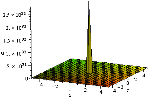
Graphical representation is an effective tool for communication and it exemplifies evidently the solutions of the problems. The graphical illustrations of the solutions are depicted in the Figures 1–2 for the MEE circular rod equation. Figure 1 is plotted for the solution (3.1.8) for the values c₀ = 2, N = 3, r = 0.50, within the interval $-5\le x,t\le 5$. The shape of the solution (3.1.8) is bell-shape soliton. For the values c₀ = −2, N = −3, r = 0.35, the solution (3.1.7) has been plotted within the interval $-5\le x,t\le 5$ and shown in Figure 2. The shape of the solution is singular soliton.

Figure 1. Bell-shaped soliton of (3.1.8) for c₀ = 2, N = 3, r = −0.50 within the interval $-5\le x,t\le 5$.

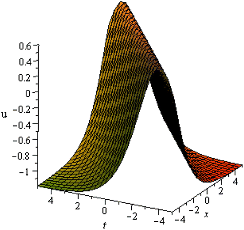
Figure 2. Singular soliton of (3.1.17) for c₀ = −2, N = −3, r = 0.35 within the interval $-5\le x,t\le 5$.

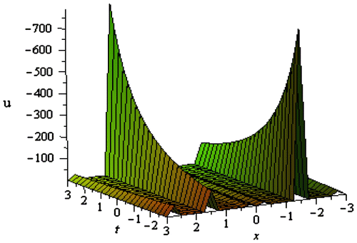
The graphical description of the solutions for the ZKBBM equation is depicted in the Figures 3–4. For the values a = 3, b = 2, r = −0.50, Figure 3 is drawn from the solution (3.2.5) within the interval $-5\le x,t\le 5$. Figure 3 represents anti-bell shape soliton. For the values a = 2, b = 5, r = 3, Figure 4 is drawn from the solution (3.2.13) within the interval $-3\le x,t\le 3$. The shape of Figure 4 is periodic.

Figure 3. Anti-bell-shaped soliton of (3.2.5) for a = 3, b = 2, r = −0.50 within the interval $-5\le x,t\le 5$.

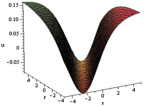
Figure 4. Periodic soliton of solution (3.2.13) for a = 2, b = 5, r = 3 within the interval $-3\le x,t\le 3$.

6. Conclusions

In this article, the improved F-expansion method combined with Riccati equation has been applied successfully to establish abundant exact traveling wave solutions to the MEE circular rod equation and the ZKBBM equation. The attained traveling wave solutions are expressed as the combination of hyperbolic, trigonometric, and rational functions. The obtained solutions are effective, useful, and practically well-suited. These solutions might be significant to illustrate some physical phenomena. The calculation procedure of this method is easy, straightforward, user friendly, and by computer algebra the method can be suitably conducted. Thus, the improved F-expansion method combined with Riccati equation can be further used to solve many other nonlinear evolution equations which often arise in various scientific real time application arenas.

Competing interests

Authors have declared that no competing interests exist.

Authors’ contributions

This work was carried out in collaboration among the authors. All authors have a good contribution to design the study and to perform the analysis of this research work. All authors read and approved the final manuscript.

Funding

The Authors received no direct funding for this research.

Acknowledgment

The authors wish to express their sincere thank to the anonymous referees, whose professional support and detailed comments help us to improve the original manuscript.

Additional information

Notes on contributors

Md. Shafiqul Islam

Md. Shafiqul Islam is a lecturer at the Department of Mathematics, Mawlana Bhashani Science and Technology University, Bangladesh. He received his BSc and MSc in Applied Mathematics from Pabna University of Science and Technology, Bangladesh in 2012 and 2013, respectively. His research interest includes nonlinear ordinary and partial differential equation, biomathematics, applied mathematics and fluid mechanics.

M. Ali Akbar

M. Ali Akbar received his PhD in Mathematics from the University of Rajshahi, Bangladesh. Currently, he is an associate professor at the Department of Applied Mathematics, University of Rajshahi, Bangladesh. His fields of interest are nonlinear differential equations and fractional calculus.

Kamruzzaman Khan

Kamruzzaman Khan received his BSc (Hons) and MSc in Applied Mathematics from University of Rajshahi, Bangladesh in 2006 and 2007, respectively. Currently, he is an assistant professor at the Department of Mathematics, Pabna University of Science and Technology, Bangladesh. His fields of interest are nonlinear ordinary and partial differential equations, fluid mechanics.

References

- Abdou, M. A. (2007). The extended tanh method and its applications for solving nonlinear physical models. Applied Mathematics and Computation, 190, 988–996.
- Akbar, M. A., & Ali, N. H. M. (2011). Exp-function method for Duffing equation and new solutions of (2+1)-dimensional dispersive long wave equations. Program in Applied Mathematics, 1, 30–42.
- Akbar, M. A., & Ali, N. H. M. (2016). An Ansatz for solving nonlinear partial differential equations in mathematical physics. SpringerPlus, 5, 24. doi:10.1186/s40064-015-1652-9
- Akbar, M. A., Ali, N. H. M., & Zayed, E. M. E. (2012). A generalized and improved (G′/G)-expansion method for nonlinear evolution equations. Mathematical Problems in Engineering, 2012, 22. doi:10.1155/2012/459879
- Ashorman, R. (2014). Multi-soliton solutions for a class of fifth-order evolution equations. International Journal of Hybrid Information Technology, 7(4), 11–18.10.14257/ijhit
- Chen, Y., & Wang, Q. (2005). Extended Jacobi elliptic function rational expansion method and abundant families of Jacobi elliptic function solutions to (1+1)-dimensional dispersive long wave equation. Chaos, Solitons & Fractals, 24, 745–757.10.1016/j.chaos.2004.09.014
- Chen, Y., & Yan, Z. (2006). The Weierstrass elliptic function expansion method and its applications in nonlinear wave equations. Chaos, Solitons & Fractals, 29(4), 948–964.10.1016/j.chaos.2005.08.071
- Cruz, H., Schuch, D., Castanos, O., & Rosas-Ortiz, O. (2015). Time-evolution of quantum systems via a complex nonlinear Riccati equation-I. Conservative systems with time-independent Hamiltonian. Annals of Physics, 360, 44–60.
- Guo, S., & Zhou, Y. (2010). The extended (G′/G)-expansion method and its applications to the Whitham-Broer-Kaup-Like equations and coupled Hirota-Satsuma KdV equations. Applied Mathematics and Computation, 215, 3214–3221.
- Islam, M. S., Khan, K., & Akbar, M. A. (2015a). An analytical method for finding exact solutions of modified Korteweg-de Vries equation. Results in Physics, 5, 131–135.10.1016/j.rinp.2015.01.007
- Islam, M. S., Khan, K., & Akbar, M. A. (2015b). The generalized Kudrysov method to solve some coupled nonlinear evolution equations. Asian Journal of Mathematics and Computer Research, 3(2), 104–121.
- Islam, M. S., Khan, K., Akbar, M. A., & Arnous, A. (2015). Generalized Kudryashov method for solving some some (3+1)-dimensional nonlinear evolution equations. New Trends in Mathematical Sciences, 3(3), 46–57.
- Islam, M. S., Khan, K., Akbar, M. A., & Mastroberardino, A. (2014). A note on improved F-expansion method combined with Riccati equation applied to nonlinear evolution equations. Royal Society Open Science, 1(2), 140038.10.1098/rsos.140038
- Jawad, A. J. M., Petkovic, M. D., & Biswas, A. (2010). Modified simple equation method for nonlinear evolution equations. Applied Mathematics and Computation, 217, 869–877.
- Khan, K., & Akbar, M. A. (2013a). Exact and solitary wave solutions for the Tzitzeica-Dodd-Bullough and the modified KdV-Zakharov-Kuznetsov equations using the modified simple equation method. Ain Shams Engineering Journal, 4, 903–909.10.1016/j.asej.2013.01.010
- Khan, K., & Akbar, M. A. (2013b). Application of exp(−Φ(ξ))-expansion method to find the exact solutions of modified Benjamin-Bona-Mahony equation. World Applied Sciences Journal, 24(10), 1373–1377.
- Khan, K., & Akbar, M. A. (2014). Exact solutions of the (2+1)-dimensional cubic Klein Gordon Equation and the (3+1)-dimensional Zakharov-Kuznetsov equation using the modified simple equation method. Journal of the Association of Arab Universities for Basic and Applied Sciences, 15, 74–81.
- Kim, H., & Sakthivel, R. (2012). New exact traveling wave solutions of some nonlinear higher-dimensional physical models. Reports on Mathematical Physics, 70, 39–50.10.1016/S0034-4877(13)60012-9
- Vitanov, N. K., & Dimitrova, Z. I. (2014). Solitary wave solutions for nonlinear partial differential equations that contain monomials of odd and even grades with respect to participating derivatives. Applied Mathematics and Computation, 247, 213–217.
- Wang, M., Li, X., & Zhang, J. (2008). The (G′/G)-expansion method and travelling wave solutions of nonlinear evolution equations in mathematical physics. Physics Letters A, 372, 417–423.10.1016/j.physleta.2007.07.051
- Wazwaz, A. M. (2008). New solutions of distinct physical structures to high-dimensional nonlinear evolution equations. Applied Mathematics and Computation, 196, 363–370.
- Xue, C. X., & Pan, E. (2013). On the longitudinal wave along a functionally graded magneto electro-elastic rod. International Journal of Engineering Science, 62, 48–55.10.1016/j.ijengsci.2012.08.004
- Yin-Long, Z., Yin-Ping, L., & Zhi-Bin, L. (2010). A connection between the (G′/G)-expansion method and the truncated Painlevé expansion method and its application to the mKdV equation. Chinese Physics B, 19(3), 030306.10.1088/1674-1056/19/3/030306
- Yusufoglu, E., & Bekir, A. (2008). Exact solutions of coupled nonlinear evolution equations. Chaos, Solitons & Fractals, 37, 842–848.10.1016/j.chaos.2006.09.074
- Zayed, E. M. E., & Gepreel, K. A. (2009). The (G′/G)-expansion method for finding the traveling wave solutions of nonlinear partial differential equations in mathematical physics. Journal of Mathematical Physics, 50, 013502–013514.10.1063/1.3033750
- Zayed, E. M. E., Zedan, H. A., & Gepreel, K. A. (2004). Group analysis and modified extended tanh function to find the invariant solutions and soliton solutions for nonlinear Euler equations. International Journal of Nonlinear Sciences and Numerical Simulation, 5, 221–234.
- Zgang, J. L., Wang, M. L., Wang, Y. M., & Fang, Z. D. (2006). The improved F-expansion method and its applications. Physics Letters A, 350, 103–109.
- Zhang, S. (2008a). Application of exp-function method to high-dimensional nonlinear evolution equation. Chaos, Solitons & Fractals, 38, 270–276.10.1016/j.chaos.2006.11.014
- Zhang, S. (2008b). Application of Exp-function method to Riccati equation and new exact solutions with three arbitrary functions of Broer-Kaup-Kupershmidt equations. Physics Letters A, 372, 1873–1880.10.1016/j.physleta.2007.10.086
- Zhang, S., & Xia, T. C. (2008). A further improved tanh function method exactly solving the (2+1)-dimensional dispersive long wave equations. Applied Mathematics E-Notes, 8, 8–66.
- Zhao, Y. M. (2013). F-expansion method and its applicationfor finding new exact solutions to the Kudryashov-Sinelshchikov equation. Journal of Applied Mathematics, 2013, 895760.