On queue with two types of general heterogeneous service with Bernoulli feedback

Abstract

This paper deals with the steady-state behavior of an M/G/1 queue with two types of general heterogeneous service to the arriving customers and Bernoulli feedback. We first derive the steady-state probability generating functions for the queue size distributions at a random epoch as well as at a departure epoch. Next, we derive the mean queue size at random epoch and the mean waiting time. Also, we obtain the mean busy period of this model and discuss some important particular cases.

Keywords:

• M/G/1 queue
• Bernoulli feedback
• steady-state probability

Public Interest Statement

As the congestion problem in teletraffic, the range of applications has grown to include not only telecommunications and computer science, but also manufacturing, air traffic control, military logistics, call centers, supermarkets, inventories, hospitals, and many other areas that involve service systems whose demands are random. The mathematical analysis of the model established the indices that presumably relate the physical and stochastic parameters to certain performance measures, such as average response and waiting time, server utilization, system throughput, probability of buffer overflow, distribution function of response and waiting time, busy period of server. The system contains sufficient detail so that its performance measures reflect the behavior of the real system.

1. Introduction

Queueing situations in which the idle server may take vacations encounter in computer, communication and manufacturing systems, etc. Many researchers have studied the vacation queueing systems in different frameworks and elaborated many applications of such vacation models.

Miller (1964) was the first to study the vacation model, where the server is unavailable for some random length of time for the M/G/1 queueing system. After Levy and Yechiali (1975) included several types of generalizations of the classical M/G/1 queueing system, this type of model has also been reported by a number of authors. When the service of a customer is unsuccessful, it may be retried again and again until a successful service completed. Takács (1963) was the first to study such a model, where the customer who completed their service are feedback instantaneously to the tail of the queue with probability p (0 ≤ p ≤ 1) or departs from the system forever with probability q{ = (1 − p)}. This mechanism is known as Bernoulli feedback. These queueing models arise in the stochastic modeling of many real life situations. For example, in data transmission, a packet transmitted from the source to the destination may be returned and it may go on until the packet is finally transmitted. Boxma and Yechiali (1997) studied such a model where the service time of the unit taken for its first service different from the subsequent service times of the unsuccessful units with gated vacations. Choi, Kim, and Choi (2003) investigated this model in more depth. Recently, Choudhury and Paul (2005) investigates an M/G/1 queueing system where the server provides two phases of general heterogeneous service and Bernoulli feedback.

2. The mathematical model

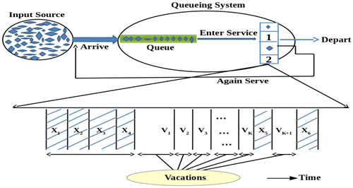
Customer arrives at the system in a compound Poisson process. There is a single server who provides two kinds of general heterogeneous one by one service to customers on a first come first served basis. Before his service starts, each customer has the option to choose the first service with probability q₁ or the second service with probability p₁ where q₁ + p₁ = 1. As soon as the system becomes empty, the server takes a vacation for a random length of time called vacation time to do other jobs, which is uninterruptible. After returning from that vacation, there are two possibilities, viz. (1) he keeps on taking vacations till he finds at least one unit in the queue (multiple vacations) or (2) he may take only one vacation between two successive busy periods (single vacation). After completion of first phase of service (FPS) or second phase of service (SPS) if the customer (unit) is not satisfied with his service for certain reason or if he received unsuccessful service, then he may immediately join the tail of the original queue as a feedback customer for receiving another regular service with probability θ (0 ≤ θ ≤ 1), otherwise he may depart forever from the system with probability θ’ (=1 − θ). Let B₁, B₂ denotes the service time of SPS and SPS, respectively (Figure 1). Assume that each of B₁, B₂ has a general distribution with distribution function B_i(x), i = 1, 2 respectively and probability density function b_i(x), Laplace Stieltzes transform (LST) $B_i^{\ast }$(s) and finite moments ${\beta }_i^{(k)}$, k ≥ 1 for i = 1, 2 (denoting FPS and SPS respectively). The model under the investigation is depicted in the Figure 1.

Figure 1. Queueing system with multiple vacation and Bernoulli feedback.

Also, let V be the vacation time random variable, v(x) be the probability density function and its distribution function is V(X) and LST is V*(s) so that the total service time required by a unit to complete the service time period is given by,$$B=\left\{\begin{array}{c}{B}_1\text{; with probability}{q}_{\text{1}}\\ B_{\text{2}}\text{; with probability}{p}_{\text{1}}\\ \end{array}\right.$$

Therefore, the LST B*(s) of B is given by,$$B^{\ast }(\text{s})=q_1{B}_1^{\ast }(\text{s})+p_1{B}_2^{\ast }(\text{s})$$

And the first two raw moments are,$${\beta }_1=q_1{\beta }_1^{(1)}+p_1{\beta }_2^{(1)}$$$${\beta }_2=q_1{\beta }_1^{(2)}+p_1{\beta }_2^{(2)}$$

3. Steady-state equations

Assume that the system is in steady state condition and define that N_Q(t) be the queue size at time t, $B_i^0$(t) be the elapsed ith types of service at time t and V⁰(t) be the elapsed vacation time at time t, i = 1, 2. Let us introduce the following random variable,$$Y(t)=\left\{\begin{array}{c}0\text{; if the system is idle at time}“t”\\ \text{1 ; if the system is busy with FPS at time}“t”\\ \text{2 ; if the system is busy with SPS at time}“t”\\ \end{array}\right.$$

Therefore, the supplementary variables $B_1^0$(t), $B_2^0$(t) and V⁰(t) are introduced in order to obtain a bivariate Markov process $\left\{N_Q\left(t\right),L(t)\right\}$, where$$L(t)=0\text{if}Y(t)=0,L(t)=V^0(t)\text{if}Y(t)=0,L(t)=B_1^0(t)\text{if}Y(t)=1,L(t)=B_2^0(t)\text{if}Y(t)=2$$

And we define,$$U(t)=\text{Prob}[N_Q(t)=0,L(t)=0]$$$$V_n(x,t)=\text{Prob}[N_Q(t)=n,L(t)=V^0(t);x<V^0\left(t\right)\le x+dx];x>0,n\ge 0$$$$P_{n,i}(x,t)=\text{Prob}[N_Q(t)=n,L(t)=B_i^0(t);x<B_i^0(t)\le x+dx];x>0,n\ge 0,i=1,2$$

Further, we assume that B_i(0) = 0, B_i(∞) = 1, V(0) = 0, V(∞) = 1, i = 1, 2 and B_i(x), V(x) are continuous at x = 0 so that μ_i(x) = $\frac{b_i(x)}{1-B_i(x)}$; i = 1,2 and therefore we have,$$b_i(\mathrm{\Omega })={\mu }_i(x)e^{-\underset{0}{\overset{\mathrm{\Omega }}{\int }}{\mu }_i(x)dx},i=1,2$$

Also ϑ(x) = $\frac{v(x)}{1-V(x)}$ and therefore v(ψ) = ϑ(x) $-\underset{0}{\overset{\psi }{\int }}$ θ(x) d(x).

Let us define the following PDF:$$P_i(x,z)=\sum _{n=0}^{\infty }{P}_{n,i}(x)z^n,P_i(z)=\sum _{n=0}^{\infty }{P}_{n,i}{z}^n,i=1,2,|z|\le 1$$$$V(x,z)=\sum _{n=0}^{\infty }{V}_n(x)z^n,V(z)=\sum _{n=0}^{\infty }{V}_n{z}^n,|z|\le 1$$

To analyze this model at stationary point of time, we can use the forward Kolmogorov equations, which under the steady-state conditions are:(1) $$\frac{d}{\mathit{dx}}{P}_{n,1}(x)+[\lambda +{\mu }_1(x)]P_{n,1}(x)=\lambda P_{n-1,1}(x),n\le 0$$(1) (2) $$\frac{d}{\mathit{dx}}{P}_{n,2}(x)+[\lambda +{\mu }_2(x)]P_{n,2}(x)=\lambda P_{n-1,2}(x),n\le 0$$(2) (3) $$\frac{d}{\mathit{dx}}{V}_n(x)+[\lambda +\vartheta (x)]V_n(x)=\lambda V_{n-1}(x),n\ge 0$$(3) (4) $$\lambda U={\theta }^{\prime }\underset{0}{\overset{\infty }{\int }}\vartheta (x)V_0(x)dx+{\theta }^{\prime }\underset{0}{\overset{\infty }{\int }}{P}_{1,0}(x){\mu }_1(x)dx+{\theta }^{\prime }\underset{0}{\overset{\infty }{\int }}{P}_{2,0}(x){\mu }_2(x)dx$$(4)

These equations are to be solved under the following boundary conditions,(5) $$P_{n,1}(0)=q_1\theta \underset{0}{\overset{\infty }{\int }}{P}_{n,1}(x){\mu }_1(x)dx+q_1{\theta }^{\prime }\underset{0}{\overset{\infty }{\int }}{P}_{n+1,1}(x){\mu }_1(x)dx+q_1\theta \underset{0}{\overset{\infty }{\int }}\vartheta \left(\text{x}\right)V_n(x)dx+q_1{\theta }^{\prime }\underset{0}{\overset{\infty }{\int }}\vartheta \left(x\right)V_{n+1}(x)dx+q_1\theta \underset{0}{\overset{\infty }{\int }}{P}_{n,2}(x){\mu }_2(x)dx+q_1{\theta }^{\prime }\underset{0}{\overset{\infty }{\int }}{P}_{n+1,2}(x){\mu }_2(x)dx,n\ge 1$$(5) (6) $$P_{0,1}(0)=q_1\underset{0}{\overset{\infty }{\int }}{P}_{1,0}(x){\mu }_1(x)dx+q_1{\theta }^{\prime }\underset{0}{\overset{\infty }{\int }}{P}_{1,1}(x){\mu }_1(x)dx+q_1\theta \underset{0}{\overset{\infty }{\int }}\vartheta \left(\text{x}\right)V_0(x)dx+q_1{\theta }^{\prime }\underset{0}{\overset{\infty }{\int }}\vartheta \left(\text{x}\right)V_1(x)dx+q_1\theta \underset{0}{\overset{\infty }{\int }}{P}_{0,2}(x){\mu }_2(x)dx+q_1{\theta }^{\prime }\underset{0}{\overset{\infty }{\int }}{P}_{1,2}(x){\mu }_2(x)dx+\lambda U{q}_1$$(6) (7) $$V_n(0)=\underset{0}{\overset{\infty }{\int }}{P}_{n,1}\left(x\right){\mu }_1(x)dx+\underset{0}{\overset{\infty }{\int }}{P}_{n,2}\left(x\right){\mu }_2(x)dx,n\ge 0$$(7) (8) $$P_{n,2}(0)=p_1\theta \underset{0}{\overset{\infty }{\int }}{P}_{n,1}(x){\mu }_1(x)dx+p_1{\theta }^{\prime }\underset{0}{\overset{\infty }{\int }}{P}_{n+1,1}(x){\mu }_1(x)dx+p_1\theta \underset{0}{\overset{\infty }{\int }}\vartheta \left(\text{x}\right)V_n(x)dx+p_1{\theta }^{\prime }\underset{0}{\overset{\infty }{\int }}\vartheta \left(\text{x}\right)V_{n+1}(x)dx+p_1\theta \underset{0}{\overset{\infty }{\int }}{P}_{n,2}(x){\mu }_2(x)dx+p_1{\theta }^{\prime }\underset{0}{\overset{\infty }{\int }}{P}_{n+1,2}(x){\mu }_2(x)dx,n\ge 1$$(8) (9) $$P_{0,2}(0)=p_1\theta \underset{0}{\overset{\infty }{\int }}{P}_{1,0}(x){\mu }_1(x)dx+p_1{\theta }^{\prime }\underset{0}{\overset{\infty }{\int }}{P}_{1,1}(x){\mu }_1(x)dx+p_1\theta \underset{0}{\overset{\infty }{\int }}\vartheta \left(x\right)V_0(x)dx+p_1{\theta }^{\prime }\underset{0}{\overset{\infty }{\int }}\vartheta \left(\text{x}\right)V_1(x)dx+p_1\theta \underset{0}{\overset{\infty }{\int }}{P}_{0,2}(x){\mu }_2(x)dx+p_1{\theta }^{\prime }\underset{0}{\overset{\infty }{\int }}{P}_{1,2}(x){\mu }_2(x)dx+\lambda U{p}_1,$$(9)

4. The steady queue size distribution

Proceeding in the usual manner with Equations (1)–(4) we obtain,(10) $$P_1(x,z)=P_1(0,z)e^{-\left(\lambda -\lambda z\right)x-\underset{0}{\overset{x}{\int }}{\mu }_1(t)dt}$$(10) (11) $$V(x,z)=V(0,z)e^{-\left(\lambda -\lambda z\right)x-\underset{0}{\overset{x}{\int }}\vartheta (t)dt}$$(11) (12) $$P_2(x,z)=P_2(0,z)e^{-\left(\lambda -\lambda z\right)x-\underset{0}{\overset{x}{\int }}{\mu }_2(t)dt}$$(12)

Solving for P₁(0,z), P₂(0,z) and V(0,z) we have(13) $$P_1(0,z)=\frac{\lambda U(z-1)q_1}{\left(1+V^{\ast }\left[\lambda -\lambda z\right]\right)\left(z\theta +{\theta }^{\prime }\right)\left(p_1{B}_2^{\ast }\left[\lambda -\lambda z\right]+q_1{B}_1^{\ast }[\lambda -\lambda z]\right)-z}$$(13) (14) $$P_2(0,z)=\frac{\lambda U(z-1)p_1}{\left(1+V^{\ast }\left[\lambda -\lambda z\right]\right)\left(z\theta +{\theta }^{\prime }\right)\left(p_1{B}_2^{\ast }\left[\lambda -\lambda z\right]+q_1{B}_1^{\ast }[\lambda -\lambda z]\right)-z}$$(14) (15) $$V(0,z)=\frac{\lambda U(z-1)\left(p_1{B}_2^{\ast }\left[\lambda -\lambda z\right]+q_1{B}_1^{\ast }[\lambda -\lambda z]\right)}{\left(1+V^{\ast }\left[\lambda -\lambda z\right]\right)\left(z\theta +{\theta }^{\prime }\right)\left(p_1{B}_2^{\ast }\left[\lambda -\lambda z\right]+q_1{B}_1^{\ast }[\lambda -\lambda z]\right)-z}$$(15)

Next from (10) and (13), we obtain,(16) $$P_1(z)=\underset{0}{\overset{\infty }{\int }}{P}_1(x,z)dx=\frac{q_1(B_1^{\ast }\left[\lambda -\lambda z\right]-1)U}{\left(1+V^{\ast }\left[\lambda -\lambda z\right]\right)\left(z\theta +{\theta }^{\prime }\right)\left(p_1{B}_2^{\ast }\left[\lambda -\lambda z\right]+q_1{B}_1^{\ast }[\lambda -\lambda z]\right)-z}$$(16)

From Equations (11) and (15), we obtain,(17) $$V(z)=\underset{0}{\overset{\infty }{\int }}V(x,z)dx=\frac{\left(p_1{B}_2^{\ast }\left[\lambda -\lambda z\right]+q_1{B}_1^{\ast }[\lambda -\lambda z]\right)\left(V^{\ast }\left(\lambda -\lambda z\right)-1\right)U}{\left(1+V^{\ast }\left[\lambda -\lambda z\right]\right)\left(z\theta +{\theta }^{\prime }\right)\left(p_1{B}_2^{\ast }\left[\lambda -\lambda z\right]+q_1{B}_1^{\ast }[\lambda -\lambda z]\right)-z}$$(17)

Also from Equations (12) and (14), we obtain,(18) $$P_2(z)=\underset{0}{\overset{\infty }{\int }}{P}_2(x,z)dx=\frac{p_1(B_2^{\ast }\left[\lambda -\lambda z\right]-1)U}{\left(1+V^{\ast }\left[\lambda -\lambda z\right]\right)\left(z\theta +{\theta }^{\prime }\right)\left(p_1{B}_2^{\ast }\left[\lambda -\lambda z\right]+q_1{B}_1^{\ast }[\lambda -\lambda z]\right)-z}$$(18)

The unknown probability U can be determined by utilizing the normalizing condition which is equivalent to, U + $P_1\left(1\right)+P_2$(1) + V(1) = 1 and the utilization factor of this system ρ is given by, ρ = 2λ$\left[q_1{\beta }_1^{(1)}+p_2{\beta }_2^{(1)}\right]$ ˂ 1, which is the steady-state probability that the system is idle and also we have $\left(\frac{\rho }{{\theta }^{\prime }}\right)$ ˂ 1; which is the stability condition under which the steady-state solution exist. Now, we let P_R(z) = U + P₁(z) + $P_2$(z) + V(z) denote the steady state PGF of the system size distribution at a random epoch, then adding the Equations (16)–(18) we obtain on simplifying,(19) $$P_R(z)=\frac{\begin{array}{c}\left[\left(3\lambda {\beta }_1+2\theta -1\right)\left(1+V^{\ast }\left[\lambda -\lambda z\right]\right)\left(z\theta +{\theta }^{\prime }\right)+\left(5\lambda {\beta }_1+2\theta -1\right)V^{\ast }\left[\lambda -\lambda z\right]\right]\\ \left(p_1{B}_2^{\ast }\left[\lambda -\lambda z\right]+q_1{B}_1^{\ast }[\lambda -\lambda z]\right)-\left[\left(3\lambda {\beta }_1+2\theta -1\right)z+\left(5\lambda {\beta }_1+2\theta -1\right)\right]\end{array}}{\left(5\lambda {\beta }_1+2\theta -1\right)\left[\left(1+V^{\ast }[\lambda -\lambda z]\right)\left(z\theta +{\theta }^{\prime }\right)\left(p_1{B}_2^{\ast }\left[\lambda -\lambda z\right]+q_1{B}_1^{\ast }[\lambda -\lambda z]\right)-z\right]}$$(19)

Let P(z) = P₁(z) + P₂(z) + V(z) be the PGF of the queue size distribution at a random epoch then,(20) $$P(z)=\frac{\left(p_1{B}_2^{\ast }\left[\lambda -\lambda z\right]+q_1{B}_1^{\ast }[\lambda -\lambda z]\right)V^{\ast }\left[\lambda -\lambda z\right]-1}{\left(1+V^{\ast }[\lambda -\lambda z]\right)\left(z\theta +{\theta }^{\prime }\right)\left(p_1{B}_2^{\ast }\left[\lambda -\lambda z\right]+q_1{B}_1^{\ast }[\lambda -\lambda z]\right)-z}$$(20)

Now, let us denote P_Q(z) as the PGF of the queue size distribution at departure epoch of this model. Then we get,(21) $$P_Q(z)=U+zP(z)=\frac{\begin{array}{c}2\left(1-2\theta -4\lambda {\beta }_1\right)z+\left(p_1{B}_2^{\ast }\left[\lambda -\lambda z\right]+q_1{B}_1^{\ast }\left[\lambda -\lambda z\right]\right)\\ \left[\left(3\lambda {\beta }_1+2\theta -1\right)\left(1+V^{\ast }\left[\lambda -\lambda z\right]\right)\left(z\theta +{\theta }^{\prime }\right)+\left(5\lambda {\beta }_1+2\theta -1\right)z{V}^{\ast }[\lambda -\lambda z]\right]\end{array}}{\left(5\lambda {\beta }_1+2\theta -1\right)\left[\left(1+V^{\ast }[\lambda -\lambda z]\right)\left(z\theta +{\theta }^{\prime }\right)\left(p_1{B}_2^{\ast }\left[\lambda -\lambda z\right]+q_1{B}_1^{\ast }[\lambda -\lambda z]\right)-z\right]}$$(21)

5. The mean queue size at a random epoch and the mean waiting time

Let L_q denote the mean queue size at a random epoch for an M/G/1 queueing system with two types of general heterogeneous service with multiple vacations and Bernoulli feedback then we obtain from (19) the mean queue size; where L_q = $\frac{d}{\mathit{dz}}$ P_q(z)|_z=1 = λ[${\mathrm{{\rm Y}}}^{(1)}$ + ${\beta }_1$]; ${\left(V^{\ast }\right)}^{\prime }[0]$ = $-{\mathrm{{\rm Y}}}^{(1)}$. We derive the LST of the waiting time distribution of a test customer for this model, to obtain this we follow the simple approach used in Kleinrock (1975) for solving the LST of the time in the system from the PGF of the distribution function of the number of the system in a regular M/G/1 queue. Let $W_q^{\ast }$(s) be the LST of the distribution function of the waiting time of a test customer of this model, then utilizing the standard argument of Kleinrock (1975) (for instance see p. 197) we may write,$$W_q^{\ast }(\lambda -\lambda z)B^{*}(\lambda -\lambda z)=P_Q(z)$$

Now, s = λ(1 − z) in the above equation we get $W_q^{\ast }$(s) and having the LST of the waiting time distribution we can easily derive the LST of the distribution function for the response time. The response time $W_R$ is the time interval from the arrival time of a tagged customer to the time when it leaves the system after service completion that means, waiting time plus service time. If $W_R^{\ast }$(s) be the LST of the distribution function of W_R then,$$W_R^{\ast }(s)=W_q^{\ast }(s)B^{\ast }(s)=\frac{\left[2\left(1-2\theta -4\lambda {\beta }_1\right)\left(1-\frac{s}{\lambda }\right)+\left(p_1{B}_2^{\ast }\left(s\right)+q_1{B}_1^{\ast }\left(s\right)\right)\left(\left(3\lambda {\beta }_1+2\theta -1\right)\left(1+V^{\ast }\left(s\right)\right)\left(1-\frac{s}{\lambda }\theta \right)+\left(5\lambda {\beta }_1+2\theta -1\right)\left(1-\frac{s}{\lambda }\right)V^{\ast }\left(s\right)\right)\right]}{\left(5\lambda {\beta }_1+2\theta -1\right)\left[\left(1+V^{\ast }\left(s\right)\right)\left(1-\frac{s}{\lambda }\theta \right)\left(p_1{B}_2^{\ast }\left(s\right)+q_1{B}_1^{\ast }\left(s\right)\right)-\left(1-\frac{s}{\lambda }\right)\right]}$$

If E$\left(W_R\right)$ be the mean response time of a test customer in this model then,$$E\left(W_R\right)=-\frac{d{W}_R^{\ast }(\text{s})}{\mathit{ds}}{|}_{s=0}.={\mathrm{{\rm Y}}}^{(1)}+{\beta }_1$$

6. Mean busy period

We obtain the mean busy period for our model. Here, we define the busy period as the length of the time interval during which the server remains busy and this continues till the instant when the server becomes free again. This busy period is equivalent to the ordinary busy period generated by the units which arrive during the vacation period plus an idle period, which we may call as generalized idle period and define,

T₀ = length of the generalized idle period

T_b = length of the busy period

Since T₀ and T_b generate an alternating renewal process, therefore, we may write,$$\frac{E\left(T_b\right)}{E\left(T_0\right)}=\frac{\text{Prob}\left[T_b\right]}{1-\text{Prob}\left[T_b\right]}$$

and, Prob [T_b] = Prob [the server is busy with FPS] + Prob [the server is busy with SPS]$$=\frac{\lambda \left(q_1{\beta }_1^{(1)}+p_1{\beta }_2^{(1)}\right)}{5\lambda {\beta }_1+2\theta -1}$$$$E(T_0)=E(V)+\frac{1}{\lambda }$$

Hence, we have E (T_b) = $\frac{{\beta }_1\left(1+\lambda E(V)\right)}{4\lambda {\beta }_1+2\theta -1}$

7. Numerical insights

Let us consider that the FPS and SPS time distributions follow exponential distribution with probability distribution function B_i(x) = 1 − $e^{(-{\mu }_{i}x)}$, x ˃ 0, i = 1, 2 with ${\beta }_i^{(1)}$ = $\frac{1}{{\mu }_i}$ and finite moment ${\beta }_i^{(2)}$ = $\frac{2}{{\mu }_i^2}$ for i = 1, 2 and the vacation time random variable follows the Erlang distribution with probability distribution function v(x) = $\frac{{\mathrm{{\rm Y}}}^{\vartheta }{x}^{\vartheta -1}{e}^{-\mathrm{{\rm Y}}x}}{\left(\vartheta -1\right)!}$, x ˃ 0 with mean $\frac{\vartheta }{\mathrm{{\rm Y}}}$.

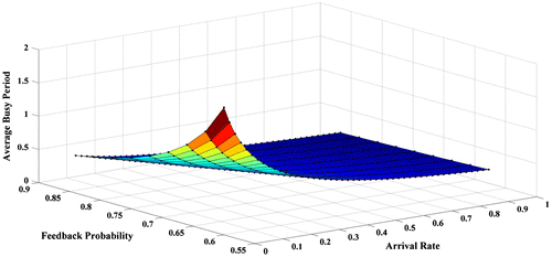
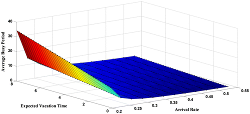
In this section, we analyze and compare the performance of the proposed model by varying the arrival rate, feedback probability and expected vacation time. We first analyze the mean busy period for the proposed queueing system with respect to the arrival rate of the customer and feedback probability. The result is graphically illustrated in Figure 2. We observed that the mean busy period decreases with the increase in arrival rate (or, feedback probability) for different values of feedback probability (or, arrival rate). Figure 3 depicts the mean busy period as the arrival rate of the customer and expected vacation time vary. A sharp increase in the busy period is observed as the expected vacation time of the server increases for fixed arrival rate of the customer. On the other hand, the expected busy period decreases with the increase in the arrival rate for fixed feedback probability.

Figure 2. Effects of arrival rate and feedback probability on the average busy period.

Figure 3. Effects of arrival rate and expected vacation time on average busy period.

The following default parameters are considered in order to find the optimal values of expected busy period as in Figures 2 and 3,

Figure 2: q₁ = 0.7, μ₂ = 2, μ₁ = 3, E(v) = 0.4

Figure 3: q₁ = 0.6, μ₂ = 2, μ₁ = 10, θ = 0.4.

8. Remarks

By specifying vacation time random variable as well as service time random variables, we obtained some results by considering some particular cases of our model.

Case I: M/$\left(\begin{array}{c}{G}_1\hfill \\ G_2\hfill \end{array}\right)$/1/V (MV) queue with Erlangian vacation time.

Suppose that vacation time is an k-Erlang, i.e. E_k with probability density function:$$v(x)=\frac{dV(x)}{\mathit{dx}}=\frac{{(kv)}^k{x}^{k-1}{e}^{-kvx}}{\left(k-1\right)!};k>0,v\ge 1$$

Also V*(λ – λz) = ${\left(\frac{\mathit{vk}}{vk+\lambda (1-z)}\right)}^k$ and E(V) = $\frac{1}{v}$, U = 1 − $\left(\frac{2\lambda {\beta }_1}{1+5\lambda {\beta }_1-2{\theta }^{\prime }}\right)$ then we have,$$P_1(z)=\frac{\left(B_1^{\ast }\left[\lambda -\lambda z\right]-1\right)q_{1}U}{\left(z\theta +{\theta }^{\prime }\right)\left({\left(\frac{\mathit{vk}}{vk+\lambda \left(1-z\right)}\right)}^k+1\right)\left(p_1{B}_2^{\ast }\left[\lambda -\lambda z\right]+q_1{B}_1^{\ast }\left[\lambda -\lambda z\right]\right)-z}$$$$V(z)=\frac{\left({\left(\frac{\mathit{vk}}{vk+\lambda \left(1-z\right)}\right)}^k-1\right)U\left(p_1{B}_2^{\ast }\left[\lambda -\lambda z\right]+q_1{B}_1^{\ast }[\lambda -\lambda z]\right)}{\left(z\theta +{\theta }^{\prime }\right)\left({\left(\frac{\mathit{vk}}{vk+\lambda \left(1-z\right)}\right)}^k+1\right)\left(p_1{B}_2^{\ast }\left[\lambda -\lambda z\right]+q_1{B}_1^{\ast }\left[\lambda -\lambda z\right]\right)-z}$$$$P_2(z)=\frac{\left(B_2^{\ast }\left[\lambda -\lambda z\right]-1\right)p_{1}U}{\left(z\theta +{\theta }^{\prime }\right)\left({\left(\frac{\mathit{vk}}{vk+\lambda \left(1-z\right)}\right)}^k+1\right)\left(p_1{B}_2^{\ast }\left[\lambda -\lambda z\right]+q_1{B}_1^{\ast }\left[\lambda -\lambda z\right]\right)-z}$$

Further from Equation (20), we get the PGF of the queue size distribution at a random epoch,$$P(z)=\frac{{\left(\frac{\mathit{vk}}{vk+\lambda \left(1-z\right)}\right)}^k\left(p_1{B}_2^{\ast }\left[\lambda -\lambda z\right]+q_1{B}_1^{\ast }[\lambda -\lambda z]\right)-1}{\left(z\theta +{\theta }^{\prime }\right)\left({\left(\frac{\mathit{vk}}{vk+\lambda \left(1-z\right)}\right)}^k+1\right)\left(p_1{B}_2^{\ast }\left[\lambda -\lambda z\right]+q_1{B}_1^{\ast }\left[\lambda -\lambda z\right]\right)-z}$$

Case II: M/$\left(\begin{array}{c}{G}_1\hfill \\ G_2\hfill \end{array}\right)$/1/V (MV) queue with Exponential vacation time.

As special case of this model, we consider the case of Markovian vacation time random variable with mean E(V) = $\frac{1}{v}$, then the PGF of the various queue size distribution of this model can be obtained by putting k = 1 in Equations (22)–(24):$$P_1(z)=\frac{\left(v+\lambda \left(1-z\right)\right)q_{1}U\left(B_1^{\ast }\left[\lambda -\lambda z\right]-1\right)}{\left(z\theta +{\theta }^{{}^{\prime }}\right)\left(\lambda \left(1-z\right)+2v\right)\left(p_1{B}_2^{\ast }\left[\lambda -\lambda z\right]+q_1{B}_1^{\ast }\left[\lambda -\lambda z\right]\right)-z\left(v-\lambda (z-1)\right)}$$$$V(z)=\frac{\lambda \left(1-z\right)U\left(p_1{B}_2^{\ast }\left[\lambda -\lambda z\right]+q_1{B}_1^{\ast }\left[\lambda -\lambda z\right]\right)}{z\left(v-\lambda \left(z-1\right)\right)-\left(z\theta +{\theta }^{\prime }\right)\left(\lambda \left(1-z\right)+2v\right)\left(p_1{B}_2^{\ast }\left[\lambda -\lambda z\right]+q_1{B}_1^{\ast }\left[\lambda -\lambda z\right]\right)}$$$$P_2(z)=\frac{\left(v+\lambda \left(1-z\right)\right)p_{1}U\left(B_2^{\ast }\left[\lambda -\lambda z\right]-1\right)}{\left(z\theta +{\theta }^{{}^{\prime }}\right)\left(\lambda \left(1-z\right)+2v\right)\left(p_1{B}_2^{\ast }\left[\lambda -\lambda z\right]+q_1{B}_1^{\ast }\left[\lambda -\lambda z\right]\right)-z\left(v-\lambda (z-1)\right)}$$

Funding

The authors received no direct funding for this research.

Additional information

Notes on contributors

Snigdha Mahanta

Gautam Choudhury is an associate professor in the Mathematical Science Division, Institute of Advanced Study in Science and Technology, Guwahati, India. There are more than 85 research publications in international/national refereed journals to his credit. His areas of interest are Queuing theory, stochastic models in the communication system and statistical inference in stochastic processes.

Gautam Choudhury

Snigdha Mahanta is a working PhD researcher in Mathematical Science Division, Institute of Advanced Study in Science and Technology, Guwahati, India. Her current research interests include the Markov chain and stochastic models in Queuing theory.

References

- Boxma, O. J., & Yechiali, U. (1997). An M/G/1 queue with multiple types of feedback and gated vacations. Journal of Applied Probability, 34, 773–784.10.1017/S0021900200101421
- Choi, B. D., Kim, B., & Choi, S. H. (2003). An M/G/1 queue with multiple types of feedback, gated vacations, and FCFS policy. Computers and Operations Research, 30(9), 1289–1309.10.1016/S0305-0548(02)00071-0
- Choudhury, G., & Paul, M. (2005). A two phase queueing system with Bernoulli feedback. International Journal of Information and Management Sciences, 16(1), 35–52.
- Kleinrock, L. (1975). Queueing systems (Vol. 1). New York, NY: Wiley.
- Levy, Y., & Yechiali, U. (1975). Utilization of idle time in an M/G/1 queueing system. Management Science, 22, 202–211.
- Takács, L. (1963). A single server queue with feedback. Bell System Technical Journal, 42, 487–503.10.1002/bltj.1963.42.issue-2
- Miller, L. W. (1964). Alternating priorities in multi-class queue (PhD dissertation). Cornell University, Ithaca, NY.