Numerical modelling of pollutant formation in a lifted methane–air vertical diffusion flame

Abstract

A comparison of turbulence and combustion models have been performed for predicting CO₂ and NO_x formation from a methane diffusion flame firing vertically upwards. The flow field has been modeled using the Reynolds-Averaged Navier–Stokes equation incorporating the k-ε realizable turbulence closure model, the k-ω shear-stress transport (SST) turbulence model and the transitional SST turbulence model and the three models have been compared. Combustion was modeled using the unsteady Stationary Laminar Flamelet Model (SLFM), the Eulerian Particle Flamelet Model (EPFM), and the Pollutant Model (PM) and the three models have also been compared. Numerical predictions show good agreement with experimental data. Furthermore, the experimental data showed that the k-ε realizable turbulence model and the k-ω SST turbulence model performed better than transitional SST model in predicting the pollutant species from the flame. The result also shows that the PM performed better than flamelet models in predicting the combustion characteristics of NO_X in the flame.

Keywords:

• gas flares
• diffusion flames
• pollutant species
• turbulence models

Public Interest Statement

According to studies, 5% of the world's natural gas production is wasted by flaring. However, this wastage cannot be compared to the environmental and health impact of gas flaring activities. The process of gas flaring releases tonnes of toxic compounds into the atmosphere and many of these compounds have been implicated as mutagens or carcinogens. Also, the IPCC (Intergovernmental Panel on Climate Change) has established that the global warming potential of methane is 25 times that of carbon dioxide. Flaring may therefore preclude the emission of methane and other greenhouse gases, although situations may arise when the toxicity of the waste gases relative to that of the products of combustion should be taken into consideration. Methane has been widely investigated in terms of emissions characteristics. This research adds to the body of literature on methane combustion using the growing field of CFD to predict the emission of pollutants, such as nitrogen oxide in methane combustion.

1. Introduction

Gas flaring is the controlled combustion of waste hydrocarbon gases from oil field and oil refinery activities due to lack of infrastructure to harness the gases. This process is associated with the undesirable formation of pollutants, such as CO, NO_x, unburned hydrocarbons, smoke as well as CO₂. Methane constitutes more than 90% of natural gas and therefore it has been widely investigated in terms of its combustion characteristics and its emissions (Flavio, Matthias, Peter, Nikolaos, & Christian, 2011; Lawal et al., 2010; Mahmud, Sangha, Costa, & Santos, 2007). Previous experiments (Brookes & Moss, 1999) have shown that that very low concentrations of soot are present in lifted methane jet diffusion flames at atmospheric pressure. This accounts for the non-luminous appearance and higher temperature in these flames as observed by Bandaru and Turns (2000). The high temperature obtained in lifted methane diffusion flames makes NOx emission of particular concern in flaring conditions. NO_x emissions have been observed to be higher in methane–air flames than in propane–air flames due to the higher flame temperatures as well as the greater entrainment of air in methane flames compared to propane flames (Lyle, Tseng, Gore, & Laurendeau, 1999; Wang, Endrud, Turns, D’Agostini, & Slavejkov, 2002).

The advances made in computing technology have enabled researchers to model the properties of turbulent jet diffusion flames using numerical techniques. In-flame temperatures and species as well as soot have been successfully modeled by several authors with good agreements with experimental data (Mahmud et al., 2007; Norton, Smyth, Miller, & SmookE, 1993; Woolley, Fairweather, & Yunardi, 2009). A previous study of variants of the k-ε turbulence closure models suggested that the realizable version is superior to the other variants in modeling diffusion flames from circular pipe burners (Lawal et al., 2010). The aim of the present work is to further extend this study by comparing the k-ε realizable turbulence closure model with the k-ε shear-stress transport (SST) turbulence model and the transitional SST turbulence model with respect to their capability in predicting a methane–air vertical diffusion flame. Three combustion models have also been investigated and compared namely: the unsteady Stationary Laminar Flamelet Model (SLFM), the Eulerian Particle Flamelet Model (EPFM), and the Pollutant Model (PM). The results of the numerical investigation were validated against experimental data obtained from the work of Yap, Pourkashanian, Howard, Williams, and Yetter (1998) with reasonably good agreement between the numerical and experimental data.

2. Numerical method

The mathematical models available in the commercial computational fluid dynamics software, Ansys-14 (2014) were used to simulate the experimental conditions. The code solves the density-averaged form of the balance equations for mass, momentum, energy, and the relevant scalar quantities describing turbulence and combustion based on the finite volume solution method.

2.1. Conservation equations

A short description of the governing equations for the analysis of turbulent reacting flows is presented below in Cartesian tensor notation.

Mass conservation:(1) $$\frac{\mathit{\partial }\overline{\mathit{\rho }}}{\mathit{\partial }t}+\frac{\mathit{\partial }}{\mathit{\partial }{x}_k}\left(\overline{\mathit{\rho }}{\tilde{u}}_k\right)=0$$(1)

Momentum conservation:

(2) $$\frac{\mathit{\partial }(\overline{\mathit{\rho }}{\tilde{u}}_i)}{\mathit{\partial }t}+\frac{\mathit{\partial }}{\mathit{\partial }{x}_k}(\overline{\mathit{\rho }}{\tilde{u}}_k{\tilde{u}}_i)=\frac{\mathit{\partial }\overline{P}}{\mathit{\partial }{x}_i}+\frac{\mathit{\partial }{\mathit{\tau }}_{ik}}{\mathit{\partial }{x}_k}+{\tilde{F}}_k-\frac{\mathit{\partial }}{\mathit{\partial }{x}_k}(\widetilde{\mathit{\rho }{u}_k^{″}{u}_i^{″}})$$(2)

where $\overline{\mathit{\rho }}$ and $\overline{P}$ are the unweighted mean density and pressure; the symbol ~ represents a Favre mean or density weighted mean quantity and the symbol ″ denotes a corresponding fluctuating quantity. The two terms on the left hand side of Equation (2) represent the accumulation and convective terms, respectively. The first three terms on the right hand side represent the pressure, viscous and source terms, respectively, while the last term represents the turbulence or Reynolds stress.

Energy conservation:(3) $$\frac{\mathit{\partial }}{\mathit{\partial }t}(\mathit{\rho }h)+\frac{\mathit{\partial }}{\mathit{\partial }{x}_j}(\mathit{\rho }h{u}_j)=\frac{\mathit{\partial }}{\mathit{\partial }{x}_j}\left(\frac{\mathit{\mu }}{Pr}\frac{\mathit{\partial }h}{\mathit{\partial }{x}_j}\right)+q_{rad}$$(3)

where h and Pr are the specific enthalpy and Prandtl number of the mixture, respectively, and q_rad is the source term due to radiation heat loss.

2.2. Turbulence models

The Reynolds stresses arising from the RANS equations were closed using the realizable k-ε turbulence model, the k-ω SST turbulence model, and the transitional SST model. The k-ε models are the most popular two-equation models for the simulation of turbulence in internal flows. The k in the equation stands for the turbulent kinetic energy, while ε stands for the turbulence frequency of the large eddies. The model is available in three forms namely: The standard k-ε, the RNG k-ε, and the realizable k-ε model. Among the reported benefit of the realizable k-ε model over, its standard version is that it more accurately predicts the spreading rate of both planar and round jets as well as providing improved predictions of the flow where boundary layers are affected by strong pressure gradients, rotation, recirculation, and separation (Shih, Liou, Shabbir, Yang, & Zhu, 1995). The modeled transport equations for k and ε in the realizable k-ε model are given by (Shih et al., 1995):(4) $$\frac{\mathit{\partial }(\mathit{\rho }k)}{\mathit{\partial }t}+\frac{\mathit{\partial }(\mathit{\rho }k{u}_j)}{\mathit{\partial }{x}_j}=\frac{\mathit{\partial }}{\mathit{\partial }{x}_j}\left[\left(\mathit{\mu }+\frac{{\mathit{\mu }}_t}{{\mathit{\sigma }}_k}\right)\frac{\mathit{\partial }k}{\mathit{\partial }{x}_j}\right]+G_k+G_b-\mathit{\rho }\mathit{\epsilon }-Y_M+S_k$$(4) (5) $$\frac{\mathit{\partial }(\mathit{\rho }\mathit{\epsilon })}{\mathit{\partial }t}+\frac{\mathit{\partial }(\mathit{\rho }\mathit{\epsilon }{u}_j)}{\mathit{\partial }{x}_j}=\frac{\mathit{\partial }}{\mathit{\partial }{x}_j}\left[\left(\mathit{\mu }+\frac{{\mathit{\mu }}_t}{{\mathit{\sigma }}_{\mathit{\epsilon }}}\right)\frac{\mathit{\partial }\mathit{\epsilon }}{\mathit{\partial }{x}_j}\right]+\mathit{\rho }{C}_{1}S\mathit{\epsilon }-\mathit{\rho }{C}_2\frac{{\mathit{\epsilon }}^2}{k+\sqrt{\mathit{\nu }\mathit{\epsilon }}}+C_{1\mathit{\epsilon }}\frac{\mathit{\epsilon }}{k}{C}_{3\mathit{\epsilon }}{G}_b+S_{\mathit{\epsilon }}$$(5)

where $G_k,G_b,Y_M$ represent the generation due to the mean velocity gradient, the generation due to buoyancy and the contribution from fluctuating dilatation, respectively. S_k and S_ɛ represent the source terms for k and ε, respectively. The values for the model constants C_1ε, C₂ σ_k and σ_ε are given by Shih et al. (1995) as 1.44, 1.9, 1.0, and 1.2, respectively. These constants have been established to ensure that the model performs optimally for certain canonical flows (Ansys theroy guide, 2014). In this paper, however, the model constant C₂ was modified to a value of 1.8 as recommended in literature (Barlow & Frank, 1998).

The k-ω models, first introduced by Wilcox (1988) are the second most widely used turbulence models after the k-ε models. The standard k-ω model solves a modified version of the k equation used in the standard k-ε model and a transport equation for the turbulence frequency, ω. The standard k-ω model is applicable to wall-bounded flows and free shear flows and includes modifications for the effects of low-Reynolds-number flows, compressibility, and shear flow spreading. A modified version of the standard k-ω model, known as the SST k-ω model was developed by Menter, Langtry, and Volker (1994) to combine the reliable formulation of the k-ω model in the near-wall region with the free-stream independence of the k-ε model in the far field. The transport equation for k and ω is given by(6) $$\frac{\mathit{\partial }(\mathit{\rho }k)}{\mathit{\partial }t}+\frac{\mathit{\partial }(\mathit{\rho }k{u}_i)}{\mathit{\partial }{x}_i}=\frac{\mathit{\partial }}{\mathit{\partial }{x}_j}\left({\mathrm{\Gamma }}_k\frac{\mathit{\partial }k}{\mathit{\partial }{x}_j}\right)+G_k-Y_k+S_k$$(6) (7) $$\frac{\mathit{\partial }(\mathit{\rho }\mathit{\omega })}{\mathit{\partial }t}+\frac{\mathit{\partial }(\mathit{\rho }\mathit{\omega }{u}_j)}{\mathit{\partial }{x}_j}=\frac{\mathit{\partial }}{\mathit{\partial }{x}_j}\left({\mathrm{\Gamma }}_{\mathit{\omega }}\frac{\mathit{\partial }\mathit{\omega }}{\mathit{\partial }{x}_j}\right)+G_{\mathit{\omega }}-Y_{\mathit{\omega }}+D_{\mathit{\omega }}+S_{\mathit{\omega }}$$(7)

where Γ_k and Γ_ω, G_k and G_ω, Y_k and Y_ω, and S_k and S_ω represent the effective diffusivity, generation, dissipation and source terms for k and ω, respectively. D_ω is the cross diffusion term. Further details on these terms are found in the ANSYS FLUENT Theory Guide.

The transition SST model is a four-equation model based on the coupling of the SST k-ω equation with two other transport equations, one for the transition onset criteria, defined by the momentum-thickness Reynolds number and one for the intermittency. The intermittency is the fraction of time that the flow is turbulent during the transition phase. This concept is used to blend the flow from laminar to turbulent regions. The transition model works with the SST turbulence model by modification of the k-ε equation and the model is appropriate for the prediction of laminar-turbulent transition of wall boundary layers.

2.3. Combustion models

The SLFM is based on the concept of a conserved scalar—the mixture fraction. In a diffusion flame comprising a fuel and oxidizer stream, the mixture fraction, Z could be defined based on the element mass fraction Y_i (Libby & Williams, 1994).(8) $$Z=\frac{Y_i-Y_{i2}}{Y_{i2}-Y_{i1}}$$(8)

where the subscripts 1 and 2 denote the oxidant and fuel streams, respectively. Therefore, at any point in the flow of the two mixing fluids, Z can be regarded as the mass fraction of the mixture originating from the fuel stream, and (Z−1) as the mass fraction originating from the oxidiser stream. Under the assumption of equal diffusivities, which is approximately the case in many practical applications, the mixture fraction does not depend on the choice of the element used for its definition. Therefore, the mixture fraction can also describe the instantaneous temperature and composition of the mixture, i.e.

(9) $${\mathit{\varphi }}_i={\mathit{\varphi }}_i(Z),\mathit{\varphi }=\mathit{\rho },T,Y_i$$(9)

where ϕ_i represents the instantaneous density, temperature or mass fraction of species, respectively. The complete laminar flamelet equation consists of a one-dimensional transport equation for the conserved scalar, the mixture fraction, and temperature. The term containing the time derivative becomes important only when there are rapid changes in the scalar dissipation rate, such as what occurs at extinction. However, if the scalar dissipation rate varies slowly enough, then the time-dependent term can be neglected. This assumption and that of unity Lewis number simplifies the SLFM equations as follows (Peters, 1984):

(10) $$\mathit{\rho }\frac{\mathit{\chi }}{2}\frac{{\mathit{\partial }}^2{Y}_i}{\mathit{\partial }{Z}^2}+{\dot{w}}_i=0$$(10)

where

(11) $$\mathit{\chi }=2D{\left(\frac{\mathit{\partial }Z}{\mathit{\partial }{x}_j}\right)}^2$$(11)

χ is the scalar dissipation rate which controls the mixing and thus links the turbulence and the chemistry of the reaction. ${\dot{w}}_i$ is the chemical source term, Y_i is the mass fraction of species i while D is the diffusion coefficient of the scalar.

The EPFM resolves the effect of the transient history of the scalar dissipation rate. The model accounts for the spatial evolution of the flamelet profile within the flow field by tracking sample fluid particles identified with unsteady flamelets. The method involves retaining the predicted fields of the scalar dissipation rate, mixture faction and its variance obtained from the unsteady flamelet equations. Using these predicted fields, an improved prediction of the averaged species mass fractions and temperature are post-processed through the solution of the so-called unsteady particle marker (flamelet) equations. The unsteady flamelet equations are solved in conjunction with a transport equation for the probability of finding a fluid particle I_I at location x and time t in the flow. The equation takes the form (Barths, Hasse, Bikas, & Peters, 2000):(12) $$\overline{\mathit{\rho }}\frac{\mathit{\partial }{\tilde{I}}_I}{\mathit{\partial }t}+\frac{\mathit{\partial }}{\mathit{\partial }{x}_j}(\overline{\mathit{\rho }}\widetilde{u_j}{\check{I}}_I)=\frac{\mathit{\partial }}{\mathit{\partial }{x}_j}\left[\frac{{\mathit{\mu }}_t}{{\mathit{\sigma }}_t}\frac{\mathit{\partial }\check{I_I}}{\mathit{\partial }{x}_j}\right]$$(12)

The PM (Hughes, Tomlin, Dupont, & Pourkashanian, 2001) on the other hand uses the well-known Zeldovich, Sadovnikov, and Frank-Kamenetskii (1947) and Fenimore and Jones (1967) mechanisms to model the thermal NO and the prompt NO, respectively. Equilibrium reaction was assumed between O and O₂, while partial equilibrium was assumed for the reactions involving OH. Experiments have shown that at high temperatures (T > 1,800 K, p = 1 atm), the reaction rates of forward and backward reactions are so fast that one obtains a partial equilibria for the reactions involving OH. However, the partial equilibrium assumption provides satisfactory results only at sufficiently high temperatures, therefore at temperatures below approximately 1,600 K, partial equilibrium may not be established because the characteristic time of combustion (given as the ratio of the flame thickness and the mean gas velocity) will be faster than the reaction time.

2.4. Radiation model

To determine the fraction of heat loss due to radiation in flames, it is necessary to solve the radiative transfer equation (RTE), which appears a sink in the energy Equation (3). The governing equation for the radiative heat transfer describes the transport of incoming and outgoing radiation intensity through the computational domain and it can be expressed as (Modest, 2003):

(13) $$\frac{dI(\overrightarrow{r},\overrightarrow{s})}{ds}+(a+{\mathit{\sigma }}_s)I(\overrightarrow{r},\overrightarrow{s})=a{n}^2\frac{\mathit{\sigma }{T}^4}{\mathit{\pi }}+\frac{{\mathit{\sigma }}_s}{4\mathit{\pi }}{\int }_0^{4\mathit{\pi }}I(\overrightarrow{r},{\overrightarrow{s}}^{\prime })\mathrm{\Phi }(\overrightarrow{s},{\overrightarrow{s}}^{\prime })d{\mathrm{\Omega }}^{\prime }$$(13)

where $\overrightarrow{r},\overrightarrow{s}$ and ${\overrightarrow{s}}^{\prime }$ are the position, direction, and scattering direction vectors, respectively. a and σ_s are the absorption and the scattering coefficient, s is the path length, n is the refractive index, I is the radiation intensity, T is the local temperature, Ф is the phase function, Ω^′ is the solid angle, and σ is the Stefan-Boltzmann constant given as 5.672 × 10⁻⁸ W/m²-K⁴.

3. Computational method

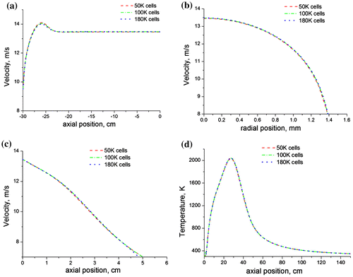
The computational simulation was based on the experimental work of (Yap et al., 1998), where they investigated a methane flame firing vertically upwards from an interchangeable fuel tube of inner diameter, d_i of 1.75 mm and outer diameter, d₀ of 3.18 mm at Reynolds number of 4,221. The simulation was achieved on a two-dimensional structured quad mesh generated using the ANSYS-ICEM meshing software. The mesh domain extended 2.3 m (700 d_i) in the axial direction and 0.4 m (123 d_i) in the radial direction (Figure 1), where d_i is the internal diameter of the pipe. 320 and 77 mesh nodes were used in the axial and radial directions, respectively, with the origin centered at the burner exit. The mesh distribution option was selected so as to place a finer node distribution in the pipe region and coarser nodes further away from the pipe (see Figure 2). A mesh refinement study was conducted to ensure the independence of the solution on the mesh size and density. This entailed comparing the velocity profiles for mesh sizes of 5 × 10⁴, 1 × 10⁵, and 2 × 10⁵ cells, respectively (Figure 3). Pressure inlet boundary conditions were employed at entrainment boundaries, located 0.3 m (92 d_i) and 0.4 m (123 d_i) away from the burner exit in the axial and radial directions, respectively. A pressure outlet boundary condition was employed at the outflow, located 2 m (615 d_i) away from the burner exit. A no-slip wall boundary condition was implemented at the pipe walls and 5% turbulence intensity was specified at the pipe inlet. The turbulence intensity at the entrainment boundaries was specified at 1 and 0.2% for the pressure inlet and outlet, respectively. Internal emissivity was set to one at all the pressure boundaries. The numerical solution was accomplished using a finite-volume discretization technique implemented in the ANSYS-Fluent solver. All the terms in the flow and combustion equations were discretized using a second-order upwind scheme, and the coupling between the pressure and velocity fields was handled via the SIMPLE algorithm implemented in the Fluent code. Activation of gravitational buoyancy in the solver had negligible effects on the predicted results. This observation has also been reported in works with similar fuel Reynold’s number (Castiñeira & Edgar, 2008; Saqr & Wahid, 2011). Residuals for all the solved equations were below 10⁻⁴ and iteration was continued until a stable residual was obtained. The kinetic of the methane reactions was modeled using the GRI mechanism (Frenklach et al., 2012) which contained 53 species with 325 reactions, while combustion was modeled with the SLFM (Peters, 1984).

Figure 1. Computational flow domain and boundary conditions.

Note: Dimensions in mm.

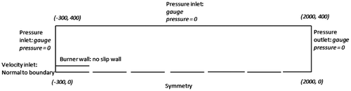
Figure 2. Hex mesh of the flow domain generated using ANSYS ICEM meshing software.

Figure 3. Predictions of (a) axial velocity, (b) radial velocity, (c) velocity at pipe exit and (d) axial temperature, for 50, 100, and 180 K mesh sizes showing meshing independence.

4. Results and discussion

4.1. Turbulence models

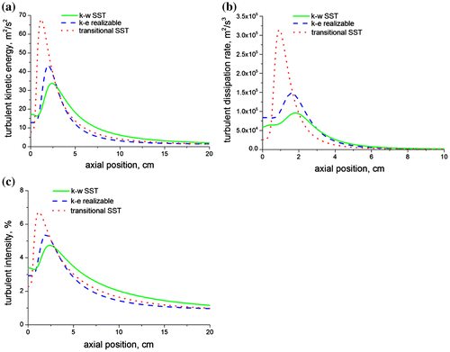
Figure 4(a–c) shows the predictions of the turbulent kinetic energy, the turbulent dissipation rate and the turbulent intensity, respectively, along the axis of the jet flame for the three turbulence models investigated. The stationary laminar flamelet combustion model was employed as a basis for comparing the three turbulence models. The transitional SST model is observed to produce a very high turbulence kinetic energy, turbulence dissipation rate, and turbulence intensity in comparison with the realizable k-ε and the k-ω SST models. The chemistry of the flame is strongly coupled with the turbulence and therefore a higher turbulent kinetic energy or turbulence intensity will increase mixing in the flame, thus leading to a faster consumption of the fuel.

Figure 4. Axial predictions of (a) turbulent kinetic energy, (b) turbulent dissipation rate and (c) turbulent intensity for a methane–air jet diffusion flame at Re = 4,221 using the three turbulence models.

This can be observed in a radial plot of the mixture fraction at three axial locations (Figure 5(a–c)) where the transitional SST severely under-predicted the concentration of methane at the flame axis when compared with the experimental data. On the other hand, the realizable k-ε and the k-ω SST models were able to capture the trend of the mixture fraction very well, especially in Figure 5(a), where we see an almost perfect fit with the experimental data. Radial predictions of the temperature and species concentration also show the superiority of the realizable k-ε and the k-ω SST models over the transitional SST, when compared with the experimental data. This is clearly visible at the first axial location (Figure 6(a)) where there is a perfect fit of the temperature predicted by the realizable k-ε with the experimental temperature measurements.

Figure 5. Radial predictions of the mean mixture fraction at (a) x/d_i = 9, (b) x/d_i = 60, and (c) x/d_i = 170 for a methane–air jet diffusion flame at Re = 4,221 using the three turbulence models.

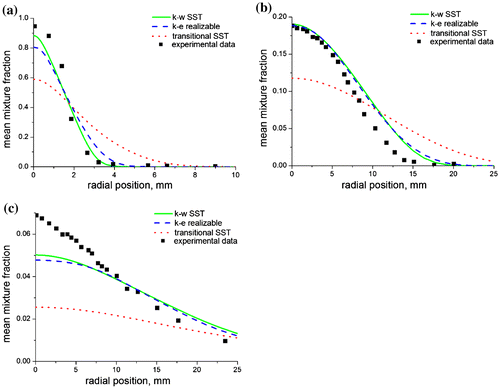
Figure 6. Radial predictions of temperature at (a) x/d_i = 9, (b) x/d_i = 60, and (c) x/d_i = 170 for a methane–air jet diffusion flame at Re = 4,221 using the three turbulence models.

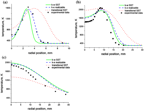
The worsening trend in the prediction of the temperature as one moves downstream of the flame can be attributed to an increase in the turbulence which leads to higher fluctuations in the temperature. Predictions of the species concentration also show good agreement with the experimental data. Nitrogen prediction (Figure 7(a–c)) is also observed to be better upstream of the flame (towards the burner nozzle), than downstream of the flame (towards the flame tip). This is because air entrainment occurs from the flame base due to the low pressure developed in this region, thus enriching the flame base with nitrogen. This increased concentration of nitrogen at the flame base leads to an improved prediction of the nitrogen concentration. On the contrary, carbon dioxide predictions (Figure 8(a–c)) are observed to be better downstream of the flame than upstream. This is because carbon dioxide is a product specie (unlike nitrogen which is a reactant), hence most of the carbon dioxide is formed at the upper section of the flame where the temperature is higher thus leading to an improved prediction in this region of the flame. Both of these observations have been confirmed by the experimental data.

Figure 7. Radial predictions of the nitrogen concentrations at (a) x/d_i = 9, (b) x/d_i = 60, and (c) x/d_i = 170 for a methane–air jet diffusion flame at Re = 4,221 using the three turbulence models.

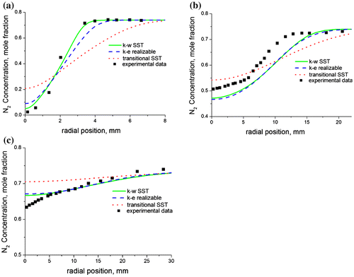
Figure 8. Radial predictions of the carbon dioxide concentrations at (a) x/d_i = 9, (b) x/d_i = 60, and (c) x/d_i = 170 for a methane–air jet diffusion flame at Re = 4,221 using the three turbulence models.

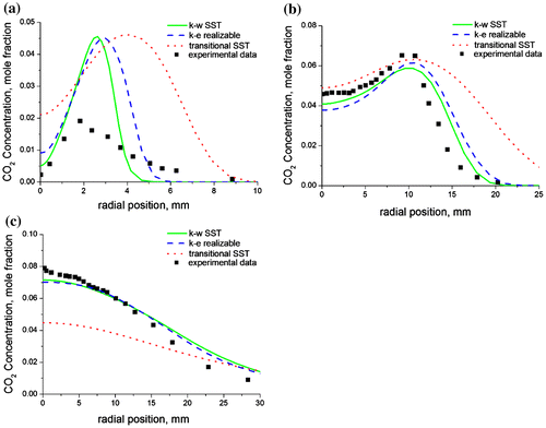
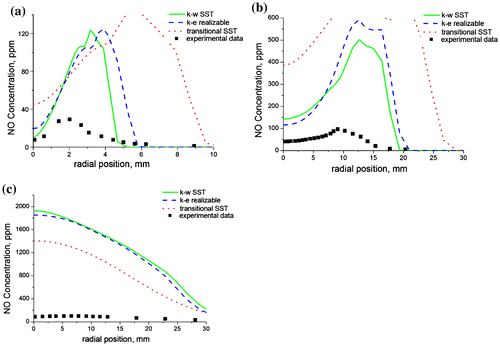
Figure 9(a–c) shows the predictions of the nitrogen oxide concentration distribution as a function of the radial position for the selected axial locations. The concentrations of nitrogen oxide in the flame are extremely small (ppm), thus making the predictions of nitrogen oxide a difficult undertaking for mathematical models. These small concentrations arise from the unreactive nature of the nitrogen molecule due to its strong triple bond which requires extremely high temperatures for bond dissociation. The flamelet models are based on a transport equation for the nitrogen oxide convection, diffusion, and production as implemented in the Fluent code. However, the flamelet equation does not account for the kinetic effects of slow forming species such as nitrogen oxide, thus making the model inadequate for nitrogen oxide predictions. This explains the poor predictions of the nitrogen oxide concentration at all the axial locations investigated.

Figure 9. Radial predictions of the nitrogen oxide concentration at (a) x/d_i = 9, (b) x/d_i = 60, and (c) x/d_i = 170 for a methane–air jet diffusion flame at Re = 4,221 using the three turbulence models.

4.2. Combustion models

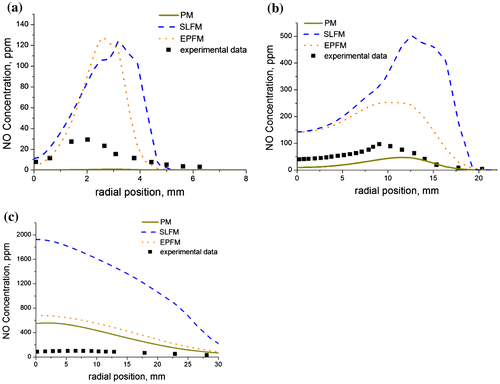
The importance of nitrogen oxide as an environmental pollutant, as well as the difficulty involved in its prediction requires accurate mathematical models. Predictions of nitrogen oxide as a function of the radial position are shown in Figure 10(a–c) for the selected axial locations using the SLFM (Peters, 1984), the EPFM (Barths et al., 2000) and the PM (Hughes et al., 2001) in an effort to compare their performances. The k-ω SST turbulence closure model has been used as a basis for the comparison, and similar results were also obtained with the k-ε realizable turbulence model. The EPFM tracks sample fluid particles identified with unsteady flamelets within the flow field, thereby accounting for the spatial evolution of the flamelet profile. This requires a converged case of a SLFM calculation which retains the predicted field of the mixture fraction and its variance as well as the scalar dissipation rate. The predicted fields are then used to obtain an improved prediction of the average temperature and the average species mass fractions through the solution of the unsteady particle marker flamelet equations. The unsteady flamelet equations are solved in tandem with a transport equation for the probability of finding a fluid particle at a given location and at a given time in the flow domain. The PM on the other hand uses the well-known Zeldovich et al. (1947) and Fenimore and Jones (1967) mechanisms to model the thermal NO and the prompt NO, respectively. Since nitrogen oxide is a slow forming species, the PM calculations for nitrogen oxide are performed after the main calculations have converged. The equations for the flamelet, radiation, and energy are deactivated in the solver and the pollutant calculation is performed until convergence is achieved. The impact of the temperature on the performance of the PM is visible from Figure 10(a) where we observe that the model could not even detect the presence of nitrogen oxide upstream of the flame at the near nozzle location (x/d_i = 9) due to the low temperature in this region of the flame. However, as we move downstream of the flame toward the mid-flame region (Figure 10(b)) where the temperature is higher, the PM begins to register the presence of nitrogen oxide. The prediction from the PM is clearly better than the predictions from the SLFM and EPFM at this particular axial location. This improved performance of the PM in comparison with the flamelet models, can be attributed to the use of a rate expression which accounts for finite rate kinetics in the NO reactions, whereas the flamelet models uses a transport equation to model the NO formation and combustion.

Figure 10. Radial predictions of the nitrogen oxide concentration at (a) x/d_i = 9, (b) x/d_i = 60, and (c) x/d_i = 170 for a methane–air jet diffusion flame at Re = 4,221 using three combustion models.

5. Conclusions

In this paper, results obtained in the numerical investigation of a turbulent methane-air jet diffusion flame have been presented and discussed and the following conclusions have been reached.

•	The realizable k-ε and the k-ω SST turbulence models performed better than the transitional SST model in predicting the temperature and species concentration from a vertical methane-air diffusion flame. The effect of gravitational buoyancy on the predicted results was also investigated and was found to negligible in the present work.
•	A comparison of the SLFM, EPFM, and the PM was made with respect to their capabilities in predicting the nitrogen oxide concentration in methane-air jet diffusion flame and the result showed that the PM performed better than the flamelet models. This has been attributed to the ability of the PM to account for finite rate kinetic effects in slow forming species, such as the oxide of nitrogen.

Funding

The author wishes to acknowledge the financial support from his sponsor, the Petroleum Technology Development Fund.

Acknowledgments

The contributions of Dr Sandy Black, Paul Crosby and Gurdev Bhogal of the University of Leeds in the UK are greatly appreciated.

Additional information

Notes on contributors

Alechenu Audu Aboje

Alechenu Audu Aboje finished his PhD in 2015 from the University of Leeds in the United Kingdom where he worked on the combustion of gases, particularly methane and propane. These two gases were selected for study due to their predominance in gas flaring, a practice that is prevalent in the oil and gas fields of Nigeria and other oil- and gas-producing nations. Other areas of interest include the application of computational fluid dynamics to the prediction of pollutants and the production and applications of alternative fuels from biomass, such as biodiesels and bioethanols. He is also a University lecturer in the Department of Chemical Engineering at the Federal University of Technology, Minna, Nigeria and teaches courses in fluid mechanics, thermodynamics and unit operations of chemical Engineering.

References

- Ansys-fluent theory guide. (2012). (Version 14.0). UK: Ansys-Fluent Sheffield.
- Bandaru, R. V., & Turns, S. R. (2000). Turbulent jet flames in a crossflow: Effects of some jet, crossflow, and pilot-flame parameters on emissions. Combustion and Flame, 121, 137–151.10.1016/S0010-2180(99)00166-2
- Barlow, R. S., & Frank, J. (1998). Effects of turbulence on species mass fractions in methane/air jet flames. 27th Symposium (international) on Combustion, 1087–1095, University of Colardo, Boulder.
- Barths, H., Hasse, C., Bikas, G., & Peters, N. (2000). Simulation of combustion in direct injection diesel engines using an Eulerian particle flamlet model. International Symposium on Combustion, 28, 1161–1168.
- Barths, H., Peters, N., Brehm, N., & Mack, A. (1998). Simulation of pollutant formation in a gasturbine combustor using unsteady flamelets. Proccedings of the Combustion Institute Institute, 27, 1841–1847.10.1016/S0082-0784(98)80026-X
- Brookes, S. J., & Moss, J. B. (1999). Measurements of soot production and thermal radiation from confined turbulent jet diffusion flames of methane. Combustion and Flame, 116, 49–61.10.1016/S0010-2180(98)00027-3
- Castiñeira, D., & Edgar, T. F. (2008). Computational fluid dynamics for simulation of wind-tunnel experiments on flare combustion systems. Energy & Fuels, 22, 1698–1706. doi:10.1021/ef700545j
- Fenimore, C. P., & Jones, G. W. (1967). Oxidation of soot by hydroxyl radicals. The Journal of Physical Chemistry, 71, 593–597.10.1021/j100862a021
- Flavio, C. C. G., Matthias, K., Peter, H., Nikolaos, Z., & Christian, B. (2011). Simulation of a lifted flame in a vitiated air environment. Proceedings of the European Combustion Meeting, 1, 12–40.
- Frenklach, M., Smith, G. P., Golden, D. M., Moriarty, N. W., & Eiteneer, B. (2012, November). GRI mechanism. Retrieved from http://www.me.berkeley.edu/gri-mech/version30/text30.html.
- Hughes, K. J., Tomlin, A. S., Dupont, V. A., & Pourkashanian, M. (2001). Experimental and modelling study of sulfur and nitrogen doped premixed methane flames at low pressure. Faraday Discussions, 119, 337–352.10.1039/b102061g
- Lawal, M. S., Fairweather, M., Ingham, D. B., Ma, L., Pourkashanian, M., & Williams, A. (2010). Numerical study of emission characteristics of a jet flame in cross-flow. Combustion Science and Technology, 182, 1491–1510. doi:10.1080/00102202.2010.496379
- Libby, P. A., & Williams, F. A. (1994). Turbulent reacting flows. California: Academic Press.
- Lyle, K. H., Tseng, L. K., Gore, J. P., & Laurendeau, N. M. (1999). A study of pollutant emission characteristics of partially premixed turbulent jet flames. Combustion Science and Technology, 116, 627–629.
- Mahmud, T., Sangha, S. K., Costa, M., & Santos, A. (2007). Experimental and computational study of a lifted, non-premixed turbulent free jet flame. Fuel, 86, 793–806.10.1016/j.fuel.2006.08.030
- Menter, F. R., Langtry, R. B., & Volker, S. (1994). Two-equation eddy-viscosity turbulence model for engineering applications. American Institute of Aeronautics and Astronautics, 32, 1598–1605.10.2514/3.12149
- Modest, M. F. (2003). Radiative heat transfer (p. 225). London: Academic Press.
- Norton, T. S., Smyth, K. C., Miller, J. H., & SmookE, M. D. (1993). Comparison of experimental and computed species concentration and temperature profiles in laminar, two dimensional methane-air diffusion flames. Combustion Science and Technology, 90, 1–34.10.1080/00102209308907601
- Peters, N. (1984). Laminar diffusion flamelet models in non-premixed turbulent combustion. Progress in Energy and Combustion Science, 10, 319–339.10.1016/0360-1285(84)90114-X
- Saqr, K. M., & Wahid, M. A. (2011). Comparison of four eddy-viscosity turbulence models in the eddy dissipation modeling of turbulent diffusion flames. International Journal of Applied Mathematics and Mechanics, 7(19), 1–18.
- Shih, T. H., Liou, W. W., Shabbir, A., Yang, Z., & Zhu, J. (1995). A new k-ε eddy viscosity model for high Reynolds number turbulent flows: Model development and validation. Computers and Fluids, 24, 227–238.10.1016/0045-7930(94)00032-T
- Wang, L., Endrud, N. E., Turns, S. R., D’Agostini, M. D., & Slavejkov, A. G. (2002). A study of the influence of, oxygen index on the soot, radiation, and emission characteristics of turbulent jet flames. Combustion Science and Technology, 174, 45–72.10.1080/00102200290021245
- Wilcox, D. C. (1988). Reassesment of the scale-determining equation for advanced turbulence models. American Institute of Aeronautics and Astronautics, 26, 1299–1310.10.2514/3.10041
- Woolley, R. M., Fairweather, M., & Yunardi, Y.. (2009). Conditional moment closure modelling of soot formation in turbulent, non-premixed methane and propane flames. Fuel, 88, 393–407. doi:10.1016/j.fuel.2008.10.005
- Yap, L. T., Pourkashanian, M., Howard, L., Williams, A., & Yetter, R. A. (1998). Nitric-oxide emission scaling of buoyancy-dominated oxygen-enriched and preheated methane turbulent-jet diffusion flames. Symposium (International) on Combustion, 27, 1451–1460.10.1016/S0082-0784(98)80552-3
- Zeldovich, Y. B., Sadovnikov, Y. P., & Frank-Kamenetskii, D. (1947). Oxidation of nitrogen in combustion. Moscow: Academy of Sciences of the USSR.