Variable selection methods for water demand forecasting in Ethiopia: Case study Gondar town

Abstract

This study developed variable selection methods to forecast urban water demand of Gondar town. Seven variable selection methods are adopted to develop appropriate water demand forecasting model. Multiple linear regression analysis was used to investigate in identifying the optimal predictor variable for developing the water demand forecasting model. The results showed that PCA played a big role to identify the influential variables in modeling of water demand in a better way as compared to other statistical methods. We developed three models to forecast the demand of water in the study area. This study selected Model 1 since Model 1 gives accurate results as compared to Model 2 and Model 3.

Keywords:

• water demand forecast
• variable selection method
• multicollinear
• Gondar town

Public Interest Statement

Water demand forecast would use to extrapolate the future demand according to the historical data of the urban water consumption as well as some correlation factor historical data. Water demand forecast can be estimated by developing appropriate mathematical models based on the predictor variables that affect the demand of water. This study developed a variable selection method to forecast urban water demand of Gondar town. The study considers monthly total rainfall (mm), number of rainy days in a month, average maximum monthly temperature, water price (US$/KL), and water restriction levels. Seven variable selection methods are adopted to develop appropriate water demand forecasting model. Multiple linear regression analysis was used to investigate in identifying the optimal predicator variable for developing the water demand forecasting model.

Competing Interest

The authors declare no conflict of interest.

1. Introduction

Water demand forecasting would use to extrapolate the future demand according to the historical data of the urban water consumption as well as some correlation factor historical data (Xinping, 2009). Accurate water demand forecast is needed for sustainable supply of water to the consumers with excellent quality, quantity and pressure (Almutaz, Ajbar, Khalid, & Ali, 2012). Water demand forecast is an important work for water resources planning and optimal allocation (Liu, Savenije, & Xu, 2003; Mohamed & Al-Mualla, 2010; Tiwari & Adamowski, 2013). Water demand forecasting can be estimated by developing appropriate mathematical models based on the predictor variables that affect the demand of water (Haque, Rahman, Hagare, & Comparative, 2018).

Climatic variables (Rainfall and Temperature), socioeconomic conditions (household income and water price), population growth, technical innovation, cost of supply and condition of water distribution system are the factors that affects the water consumption pattern of the town (Anele, Todini, Hamam, & Abu-Mahfouz, 2018). Identification of crucial variable is essential for the development of the water demand forecasting model since the accuracy of the model depends on the selection of suitable sets of predictor variables. These variables are strongly correlated each other which can create multicollinearity problems during the regression-based model development (Haque et al., 2018).

There are various methods for water demand forecasting. The most commonly used methods for water demand forecast are: the water quota approach, the conventional tendency approach, multiple linear regression approach, system dynamics approach, the gray model approach and artificial neural network approach (Ghalehkhondabi, Ardjmand, Ii, & Weckman, 2017; Objectives, 2017; Russo, Alfredo, & Fisher, 2014; Sebri, 2016; Wang, Lei, Guo, You, & Wang, 2015; Worqlul, Collick, Rossiter, Langan, & Steenhuis, 2015). Recently, linear regression model has been adopted by many researchers to develop water demand forecasting models (Al-Musaylh, Deo, Adamowski, & Li, 2018; Bakker, Duist, Van, Schagen, Van, Vreeburg, & Rietveld, 2014; Britz, Ferris, & Kuhn, 2013; Candelieri et al., 2018; Gustin, Mcleod, & Lomas, 2018; Quilty & Adamowski, 2018; Sebri, 2016). Donkor et al. (Haque et al., 2018) stated that neural networks and hybrid models are more suitable for short-term water demand forecasting, while regression-based models are more appropriate for long-term forecasting.

In our paper, we choose the variable selection methods to choose the best variable selection methods to predict the urban water demand of Gondar town. Thus, our paper aims to compare the different variable selection methods regarding elimination of the multicollinearity problems in the linear regression model in line with water demand forecasting. The selected variables for prediction of water demand depend on the time horizon such as short-term and long-term water demand forecasting. Seven variable selection methods are nominated in our study to find the optimal variable to set in the development of the time horizon models in water demand forecasting. The variable selection methods compared are (1) Forward selection (FS); (2) Backward Elimination (BW); (3) Stepwise selection (SW); (4) Residual mean square error (MSE); (5) Mallow’s CP criterion (CP); (6) Akaike Information Criterion (AIC) and (7) Principal component analysis (PCA). The target of variable selection procedure is to identify the right predictor variables that have a great impact on the response variable and provide robust model prediction. Many studies so far have been done on variable selection methods on different disciplines (Araujo, Peres, & Fogliatto, 2017; Duan et al., 2018; Figueiredo, De, Cordella, Bouveresse, Rutledge, & Archer, 2018; Gilhodes et al., 2017; Herrera, 2010; Rahman, Imtiaz, & Hawboldt, 2016; Sheng et al., 2018; Zubaidi et al., 2018). However, the number of studies by variable selection methods on water demand forecasting is very limited. Therefore, this paper tried to fill the gap to forecast the water demand by choosing seven variable selection methods.

The findings of this paper are expected to provide base information about variable selection methods in modeling of water demand forecasting for accurate prediction.

2. Materials and methods

2.1. Study area

Gondar town is found in Northern Ethiopia which lies 12°30ʹ North and 37°20ʹ East. The town is located at an altitude of 1500–2200 m above sea level. The maximum and minimum temperatures of the area were 30.7 °C and 12.3 °C, respectively. The area receives a bimodal rainfall pattern with an annual precipitation rate of 1000 mm (Garedew, Hagos, Zegeye, & Addis, 2015).

2.2. Data sources

The raw data used in this study are monthly total rainfall (mm), number of rainy days in a month, average maximum monthly temperature, water price (US$/KL), and water restriction levels. These are obtained from National Meteorological Agency of Ethiopia.

2.3. Methods

For modeling the residential water demand forecasting, seven variable selection methods were adopted in this study to identify the predictor variables. These methods were evaluated by using a split sample validation methods (Mekasha, Tesfaye, & Duncan, 2014). The study period was divided into two parts (January 2010 to December 2015) to develop the multiple linear regression models (MLR) and from (January 2016 to December 2017) to validate the developed models. The MLR technique develops a model by constructing a linear relationship between two or more independent variables with a dependent variable and expressed as follows:

(1) $Y=b_0+b_1{x}_1+b_2{x}_2+...+b_i{x}_i+\epsilon$(1)

where Y is the dependent variable, $b_0$ … $b_i$ are the coefficients estimated by the least squares method, x₁ … x_i are the independent variables, i is the number of independent variables and $\epsilon$ is the error term related to each observation. The semi-log form was considered to develop the multi-linear regression models in this paper by using seven variable selection methods. In this paper, the dependent variable was taken in the logarithmic form and the independent variables were incorporated. The seven variable selection methods are described as follows.

2.3.1. Forward selection (FS)

FS method adds variables to the model until no remaining variable (outside the model) can add anything significant to the dependent variable. FS begins with no variable in the model. For each variable, the test statistic (TS), a measure of the variable’ s contribution to the model, is calculated. If the calculated p-value for the variable is found to be less than the critical value, then the FS method keeps the variable in the model, otherwise the variable is removed from the model. This is done literatively until all the variables in the model have a value of p < 0.1. The partial F-statistic was calculated by Equation (2) and compared with F- distribution to estimate the p-value. A critical threshold value of p < 0.1 was adopted in this study:

(2) $Fi=\frac{\left(SS{E}_{i-1}-SS{E}_i\right)\mathrm{x}\mathrm{n}-\mathrm{k}-1}{SS{E}_i\mathrm{k}}$(2)

where SSE_i–1 and SSE_i are the sum of square errors before and after the exclusion of a predictor variable, n is the number of data points, and k is the number of predictor variables.

2.3.2. Backward elimination (BE)

This is the simplest of all variable selection procedures and can be easily implemented without special software. This method deletes variables one by one from the model until all remaining variables contribute something significant to the dependent variable. BE begins with a model that includes all variables (Mekasha et al., 2014). Variables are then deleted from the model one by one until all the variables remaining in the model have the TS values greater than the present value. In situations where there is a complex hierarchy, backward elimination can be run manually while taking account of what variables are eligible for removal. It starts with all the predictors in the model and remove the predictor with highest p-value greater than the critical value

2.3.3. Stepwise selection (SW)

This is a combination of backward elimination and FS. This addresses the situation, where variables are added or removed early in the process. At each stage, a variable may be added or removed and there are several variations on exactly how this is done. Stepwise procedures are relatively cheap computationally. Like the FS method, it starts with no variable in the model, and variables are added one by one to the model by fulfilling the p criteria (p < 0.1). After a variable is added in the model, the stepwise selection method investigates all the variables in the model and deletes any variable that show a p-value greater than the critical value. The next variable is added in the model only after checking the model and deleting any variables if necessary (Haque et al., 2018). This process continues till none of the variables outside the model have a p-value less than the critical value and every single variable in the model satisfies the p criteria.

2.3.4. Mean square error (MSE)

This method finds several subsets of different sizes that best predict the dependent variable. R² finds subsets of variables that best predict the dependent variable based on the appropriate TSs. If there are k potential predictor variables, then the possible number of prediction models would be 2^k. The independent variables were considered and with MSE criteria, all the possible models were evaluated and the model with the lowest value of MSE was selected. The MSE measures the variance for each of the models and is equated as follows:

(3) $MSE=\frac{\sum {\left(Y-Yp\right)}^2}{\mathrm{n}-\mathrm{p}}$(3)

where Y and Yp are the observed and predicted water demand value, respectively, n is the number of data points, and k is the number of independent variables.

2.3.5. Best model with the Akaike information criterion (AIC)

The AIC procedure was proposed by Akaike (Haque et al., 2018), and it selects the model with the minimum value of the AIC, which can be calculated by the following equation:

(4) $AIC=nlog\left(MSE\right)+2k$(4)

2.3.6. Best model with mallow’s cp criterion (CP)

The Cp criterion was proposed by Mallow (Look, 2010) for univariate regression analysis, and it selects the model with the minimum value of the Cp statistic. The Cp statistic can be calculated as follows:

(5) $\mathrm{C}\mathrm{p}=\frac{\left(SS{E}_k\right)}{S^2}-\left(n-2k\right)$(5)

where S² is the MSE for the full model and SSE_k is the residual sum of squares for the subset model that contains k number of predictor variables in the model.

2.3.7. Principal component analysis (PCA)

Principal component analysis is one of the most frequently used multivariate data analysis methods. It is a projection method as it projects observations from a p-dimensional space with p variables to a k-dimensional space (where k < p) so as to conserve the maximum amount of information (information is measured here through the total variance of the dataset) from the initial dimensions. PCA dimensions are also called axes or factors.

If the information associated with the first 2 or 3 axes represents a sufficient percentage of the total variability of the scatter plot, the observations could be represented on a two- or three-dimensional chart, thus making interpretation much easier.

(6) $PC1=b_{11}{x}_1+b_{12}{x}_2+...+b_{1k}{x}_k=\sum _{j=1}^k{b}_{1j}{x}_j$(6)

(7) $PC1=b_{21}{x}_1+b_{22}{x}_2+...+b_{2k}{x}_k=\sum _{j=1}^k{b}_{2j}{x}_j$(7)

where x₁, x₂,..x_k represent the original variables in the data matrix and b_ij represent the eigenvectors.

3. Results

3.1. Standardized coefficients of the variable selection methods

The standardized coefficient indicates how much the effect of each independent variables on the dependent variable in our results. The results showed that out of the five variables (rainfall, maximum temperature, number of rainy days, water price and water restriction zone) three variables are statistically significant in FS, four in BE, three in SE and four MSE variable selection methods (Figure 1). Rainfall was the most influential variables in our study for water demand forecasting.

Figure 1. Coefficients of the independent variables for each variable selection method.

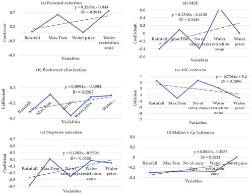
The results showed that rainfall, maximum temperature, number of rainy days and water restriction zone had no any significant impact on water demand forecast by Mallow’s Cp criterion and AIC variable selection methods. However, the results of these variables by Mallow’s Cp criterion methods are negative. Maximum temperature showed a negative result by AIC methods. It is clearly seen in (Figure 1) and (Table 1) that all the variable selection methods show a different result and takes different sets of variables to be taken as an input in the linear regression models. The results also showed that the relation between the variable selection methods and water demand was irrational. This is due to the presence of multicollinearities among the independent variables (Haque et al., 2018).

Table 1. Modeling results from the developed models adopting different variable selection methods

Model	FS		BW		SW		MSE		Mallow’s Cp	AIC
N	17		17		17		17		17	17
Independent variable	Cf.	P-value	Cf.	P-value	Cf.	P-value	Cf.	P-value	Cf.	Cf.
Constant	5.235	0.00	6.014	0.004	5.235	0.000	–	0.004	–	–
Rainfall	−0.664	0.021	−0.488	0.120	−0.664	0.021	−0.397	0.120	−0.303	5.543
Maximum temperature	0.117	0.628	0.086	0.106	0.117	0.127	0.096	0.679	−0.280	−0.071
No. of rainy days	0.400	0.061	−0.611	0.061	−0.400	0.464	−0.391	0.087	−0.267	5.631
Water price	–	–	–	–	–	–	–	–	–	–
Water restriction zone	0.071	0.758	0.052	0.768	0.071	0.081	0.65	0.768	−0.275	3.251

Note: Cf = coefficient.

As far as modeling statistical results concerned, the best model was selected based on the value of R² and adjusted R² value. Hence, the highest value of R² and adjusted R² are the best model. The findings of this paper showed that the highest value of R² is recorded in Model 2 and found to be the best model (Table 2).

Table 2. Modeling performance by applying the different variable selection methods

Model	R^2	Adjusted R^2
Model 1	45%	28%
Model 2	45%	33%
Model 3	44%	37%

3.2. Pearson’s correlation matrices of the water demand variables

The results of the Pearson’s correlation matrices of the water demand showed that the maximum correlation coefficient was found to be 0.318 between water price and maximum temperature followed by 0.222 between number of rainy days and rainfall. All the correlation results are found in Table 3. However, the presence of high correlation between independent variables indicates a strong multicollinearity, which is more likely to produce biased results in the regression analysis.

Table 3. Pearson’s correlation matrix of the independent variables

Variables	Rainfall	Max. Tem	No. of rainy days	Water price	Water restriction zone
Rainfall	1	−0.408	0.222	−.541*	−0.274
Max. temperature		1	−0.155	0.318	−0.008
No. of rainy days			1	−.500*	−0.104
Water price				1	0.214
Water restriction zone					1

3.3. Principal component analysis (PCA)

The eigenvalues of each principal component analysis on the independent variables are shown in Figure 2. The results showed that 60% of the last three principal components (PCs) show variability. The eigenvalues of the three PCs are less than one. Therefore, this paper selected PC-1 to PC-5 which were chosen to find the influencing variables to estimate the water demand. Bold values indicate a correlation between PCs and independent variables (Table 4). This study incorporated all the independent variables in the chosen five PCs.

Table 4. Correlation matrix of the independent variables by PCA

Variables	Rainfall	Max. Tem	No. of rainy days	Water price	Water restriction zone
Rainfall	1.000	−0.356	0.410	−0.480	−0.411
Max. tem	−0.356	1.000	−0.445	0.284	0.000
No. of rainy days	0.410	−0.445	1.000	−0.456	0.000
Water price	−-0.480	0.284	−0.456	1.000	0.164
Water restriction zone	−0.411	0.000	0.000	0.164	1.000

Figure 2. Eigen values of the principal components.

Hence, the independent variables heavily loaded in PC-1 are rainfall, maximum temperature; in PC-2 are rainfall, maximum temperature and number of rainy days; in PC-3 the loaded variables are maximum temperature, number of rainy days and water price; in PC-4 number of rainy days, water price and water restriction zones and in PC-5 the loaded independent variables are number of rainy days, water price and water restriction zones. However, since PC-1 and PC-2 are mostly occupied by rainfall and maximum temperature variables and highly correlated with each other. Therefore, they are chosen from PC-1 to use in regression analysis to avoid the multicollinearity problem.

Finally, we developed three individual models by using the independent variables by considering the loading potentials with the principal component analysis. These models are 1, 2, and 3. The potentials of each model indicated in Table 2.

1. Model 1: Rainfall, maximum temperature, number of rainy days, water restriction zone

2. Model 2: Rainfall, maximum temperature, number of rainy days

3. Model 3: Rainfall, number of rainy days

When we developed the three models, the water price zones in all models were not found to be statistically significant by using regression analysis. Therefore, we ignored this variable in the three models during simulation results of the models.

From the results, we can conclude that Model 1 gives better results as compared with the other two models. Models 2 and 3 give weak results. This may be due to multicollinearity problem of the variables (Haque et al., 2018) (Table 5). The most influencing predictor variables for determining the water demand in Gondar town were rainfall, maximum temperature, number of rainy days and water restriction zone. The results show that the chosen independent variables are performing good accuracy of water demand prediction and the developed model is free from the multicollinearity problem. This method is also simple to apply for water demand forecast in water supply system.

Table 5. The three developed model results by principal component analysis

Model	Model 1		Model 2		Model 3
Independent variables	Cf	P-value	Cf	P-value	Cf	P-value
Constant	6.014	0.004	6.271	0.001	6.688	0.000
Rainfall	−0.488	0.120	−0.513	0.079	−0.555	0.037
Maximum temperature	0.153	0.679	0.137	0.679	–	–
Number of rainy days	−0.611	0.087	−0.617	0.073	−0.626	0.61
Water restriction	0.069	0.789	–	–	–	–

4. Conclusion

This study analyzed and compared the results of the FS, backward elimination, stepwise selection, MSE criterion, Mallow’s Cp criterion, AIC and PCA variable selection methods for water demand forecasting of Gondar town. The results indicate that the seven variable selection methods resulted in different sets of predictor variables.

The result showed that PCA played a major role to identify the influential variables in modeling of water demand in a better way as compared to other statistical methods. The results of this study are exactly fit with the study area in Ethiopia and hence other areas can also adopt the developed system having different water consumption pattern and climate conditions to develop water demand forecasting models. The results of this paper also indicated that incorporating many independent variables in the model could not necessarily improve the performance efficiency of the models.

Acknowledgments

The authors thank the National Meteorological Service Agency of Ethiopia for providing the raw data. The authors also thank China Institute of Water Resources and Hydropower Research for financing this research.

Additional information

Funding

This work was supported by National Key Research and Development Project [grant number 2016YFA0601503].

Notes on contributors

Mohammed Gedefaw

We submitted a manuscript entitled: “Variable selection methods for water demand forecasting in Ethiopia: Case study Gondar town” which will be published in Cogent Environmental Science journal. All authors certify that they have participated sufficiently in the work to take public responsibility for the content, including participation in the concept, design, analysis, writing, or revision of the manuscript. For example, Dr. Mohammed Gedefaw is the principal author of this paper and made substantial contributions to the design, idea generating, analysis, interpretation and drafting of the manuscript. All the other co-authors greatly contributed for the improvement of the paper. This paper is under water and natural resources management research thematic team. The final manuscript before submission was checked and approved by all the authors.

References

- Al-Musaylh, M. S., Deo, R. C., Adamowski, J. F., & Li, Y. (2018). Advanced engineering informatics short-term electricity demand forecasting with MARS, SVR and ARIMA models using aggregated demand data in Queensland, Australia. Advanced Engineering Informatics, 35, 1–16. doi:10.1016/j.aei.2017.11.002
- Almutaz, I., Ajbar, A., Khalid, Y., & Ali, E. (2012). A probabilistic forecast of water demand for a tourist and desalination dependent city : Case of Mecca, Saudi Arabia. DES, 294, 53–59. doi:10.1016/j.desal.2012.03.010
- Anele, A. O., Todini, E., Hamam, Y., & Abu-Mahfouz, A. M. (2018). Predictive uncertainty estimation in water demand. 12–15. doi:10.3390/w10040475
- Araujo, F., Peres, P., & Fogliatto, F. S. (2017). Variable selection methods in multivariate statistical process control: A systematic literature review. Computation Industrial Engineering. doi:10.1016/j.cie.2017.12.006
- Bakker, M., Duist, H., Van Schagen, K., Van Vreeburg, J., & Rietveld, L. (2014). Improving the performance of water demand forecasting models by using weather input. Procedia Engineering, 70, 93–102. doi:10.1016/j.proeng.2014.02.012
- Britz, W., Ferris, M., & Kuhn, A. (2013). Environmental modelling & software modeling water allocating institutions based on multiple optimization problems with equilibrium constraints. Environmental Modelling and Software, 46, 196–207. doi:10.1016/j.envsoft.2013.03.010
- Candelieri, A., Giordani, I., Archetti, F., Barkalov, K., Meyerov, I., Polovinkin, A., … Zolotykh, N. (2018). Tuning hyperparameters of a SVM-based water demand forecasting system through parallel global optimization. Computers and Operations Research, 1–8. doi:10.1016/j.cor.2018.01.013.
- Duan, F., Fu, X., Jiang, J., Huang, T., Ma, L., & Zhang, C. (2018). Spectrochimica Acta Part B automatic variable selection method and a comparison for quantitative analysis in laser-induced breakdown spectroscopy. Spectrochim Acta Particle B Atomic Spectroscopic, 143, 12–17. doi:10.1016/j.sab.2018.02.010
- Figueiredo, M., De, Cordella, C. B. Y., Bouveresse, D. J., Rutledge, D. N., & Archer, X. (2018). Chemometrics and intelligent laboratory systems a variable selection method for multiclass classi fi cation problems using two-class ROC analysis. Experimental Eye Research, 177, 35–46. doi:10.1016/j.exer.2018.07.029
- Garedew, L., Hagos, Z., Zegeye, B., & Addis, Z. (2015). The detection and antimicrobial susceptibility profile of Shigella isolates from meat and swab samples at butchers ’ shops in Gondar town, Northwest. Journal Infection Public Health. doi:10.1016/j.jiph.2015.10.015
- Ghalehkhondabi, I., Ardjmand, E., Ii, W. A. Y., & Weckman, G. R. (2017). Water demand forecasting : Review of soft computing methods. Environmental Monitoring and Assessment, 189. doi:10.1007/s10661-017-6030-3
- Gilhodes, J., Zemmour, C., Martinez, A., Delord, J., Leconte, E., Boher, J., & Filleron, T. (2017). Comparison of variable selection methods for high-dimensional survival data with competing events. 91, 159–167. doi:10.1016/j.compbiomed.2017.10.021.
- Gustin, M., Mcleod, R. S., & Lomas, K. J. S. C. (2018). Build Environment. doi:10.1016/j.buildenv.2018.07.045
- Haque, M., Rahman, A., Hagare, D., & Comparative, A. (2018). Assessment of variable selection methods in urban water demand forecasting. 1–15. doi:10.3390/w10040419
- Herrera, M. (2010). Predictive models for forecasting hourly urban water demand, 387, 141–150. doi:10.1016/j.jhydrol.2010.04.005.
- Liu, J., Savenije, H. H. G., & Xu, J. (2003). Forecast of water demand in Weinan City in China using WDF-ANN model. 28, 219–224. doi:10.1016/S1474-7065(03)00026-3.
- Look, A. C. (2010). Variable selection methods in regression : Ignorable problem, outing. 18, 65–75. doi:10.1057/jt.2009.26.
- Mekasha, A., Tesfaye, K., & Duncan, A. J. (2014). Trends in daily observed temperature and precipitation extremes over three Ethiopian eco-environments. International Journal Climatology, 34, 1990–1999. doi:10.1002/joc.2014.34.issue-6
- Mohamed, M. M., & Al-Mualla, A. A. (2010). Water demand forecasting in Umm Al-Quwain using the constant rate model. DES, 259, 161–168. doi:10.1016/j.desal.2010.04.014
- Objectives, E. (2017). Optimal use of agricultural water and land resources through reconfiguring crop planting structure under socioeconomic and. doi:10.3390/w9070488
- Quilty, J., & Adamowski, J. (2018). Addressing the incorrect usage of wavelet-based hydrological and water resources forecasting models for real-world applications with best practices and a new forecasting framework. Journal of Hydrology, 563, 336–353. doi:10.1016/j.jhydrol.2018.05.003
- Rahman, M., Imtiaz, S. A., & Hawboldt, K. (2016). Chemometrics and intelligent laboratory systems a hybrid input variable selection method for building soft sensor from correlated process variables. Chemom Intelligent Laboratory Systems, 157, 67–77. doi:10.1016/j.chemolab.2016.06.015
- Russo, T., Alfredo, K., & Fisher, J. (2014). Sustainable water management in urban, agricultural, and natural systems. 3934–3956. doi:10.3390/w6123934
- Sebri, M. (2016). Forecasting urban water demand : A meta-regression analysis. Journal of Environmental Management, 183, 777–785. doi:10.1016/j.jenvman.2016.09.032
- Sheng, C., Miaw, W., Assis, C., Rangel, A., Sales, C., Cunha, M. L., … Carvalho, S. V. 2018. Determination of main fruits in adulterated nectars by ATR-FTIR spectroscopy combined with multivariate calibration and variable selection methods. Food Chemistry. doi:10.1016/j.foodchem.2018.02.015
- Tiwari, M. K., & Adamowski, J. (2013). Urban water demand forecasting and uncertainty assessment using ensemble wavelet-bootstrap-neural network models. 49, 6486–6507. doi:10.1002/wrcr.20517.
- Wang, X., Lei, X., Guo, X., You, J., & Wang, H. A. O. (2015). Forecast of irrigation water demand considering multiple factors. 331–336. doi:10.5194/piahs-368-331-2015
- Worqlul, A. W., Collick, A. S., Rossiter, D. G., Langan, S., & Steenhuis, T. S. (2015). Catena assessment of surface water irrigation potential in the Ethiopian highlands : The Lake Tana Basin. Catena, 129, 76–85. doi:10.1016/j.catena.2015.02.020
- Xinping, X. (2009). The research on forecasting water demand methods for Changzhi City in Shanxi Province, (4), 5261–5264.
- Yesuf, M., Kassie, M., & Köhlin, G. (2009). Environment for development risk implications of farm technology adoption in the Ethiopian Highlands.
- Zubaidi, S. L., Dooley, J., Alkhaddar, R. M., Abdellatif, M., Al-Bugharbee, H., & Ortega-Martorell, S. (2018). A novel approach for predicting monthly water demand by combining singular spectrum analysis with neural networks. Journal of Hydrology, 561, 136–145. doi:10.1016/j.jhydrol.2018.03.047