Determining farm-scale site-specific monetary values of “soil carbon hotspots” based on avoided social costs of CO₂ emissions

Abstract

A “soil carbon hotspot” (SCH) is a geographic area having an abundance of soil carbon, and therefore higher ecosystem services value based on avoided social costs of CO₂ emissions. Soil organic carbon (SOC), soil inorganic carbon (SIC), and total soil carbon (TSC) are critical data to help identify SCH at the farm scale, but monetary methods of hotspot evaluation are not well defined. This study provides a first of its kind quantitative example of farm-scale monetary value of soil carbon (C), and mapping of SCH based on avoided social cost of CO₂ emissions using both Soil Survey Geographic (SSURGO) database and field measurements. The total calculated monetary value for TSC storage at the Willsboro Farm based on the SSURGO database was about 7.3 million U.S. dollars ($7.3 M), compared to $2.8 M based on field data from averaged soil core results. This difference is attributed to variation in soil sampling methodology, laboratory methods of soil C analyses, and depth of reported soil C results. Despite differences in total monetary valuation, observed trends by soil order were often similar for SSURGO versus field methods, with Alfisols typically having the highest total and area-normalized monetary values for SOC, SIC, and TSC. Farm-scale C accounting provides a more detailed spatial resolution of monetary values and SCH, compared to estimates based on country-level reports in soil survey databases. Delineation and mapping of SCH at the farm scale can be useful tools to define land management zones, to achieve social profit for farmers, and to realize United Nations (UN) Sustainable Development Goals (SDGs) based on avoided social cost of CO₂ emissions.

Keywords:

• ecosystem services (ES)
• external costs
• hotspots
• hot moments
• social profit
• soil organic carbon (SOC)
• soil inorganic carbon (SIC)
• total soil carbon (TSC)
• SSURGO

PUBLIC INTEREST STATEMENT

A “soil carbon hotspot” (SCH) is a geographic area having an abundance of soil carbon, and therefore higher ecosystem services value based on avoided social costs that would arise from CO₂ emissions. This study analyzed differences in monetary values of this avoided social cost at the farm scale using a soil survey database and comparing it to detailed field measurements. Social cost estimates using the soil survey database were higher than the farm-specific field measurements by almost 2.6 times. These differences in values can be attributed to the limitations of the soil survey information which can be used at the county, state, and regional levels. Field data provided a greater detail in identifying and delineating these carbon hotspots within the farm. The proposed method to identify SCH can be applied to the farms with different types of soil carbon due to geographic differences. It can be also incorporated with precision agriculture to enhance a decision support system to ensure both agricultural profitability and sustainability.

Competing Interests

The authors declare no competing interests.

1. Introduction

Agriculture (e.g., farms) is one of many beneficiaries from ecosystem services (ES) provided by soil organic carbon (SOC), soil inorganic carbon (SIC), and total soil carbon (TSC) stored in the pedosphere (mixed ownership) and atmosphere (common-pool resource), and transforms its stocks and flows into various commodities with identified market value (Figure 1). Atmospheric carbon dioxide (CO₂) is absorbed by plants, which are harvested from the farm with some of the carbon (C) being removed in these harvested products, and some of it is returned to the soil as soil organic matter (Bhattacharyya et al., 2014; Franzluebbers et al., 2006). This transformation alters soil regulating ES (e.g., gas regulation, etc.) and can be accompanied by greenhouse gas (GHG) emissions (e.g., CO₂, etc.) into the atmosphere, and/or C sequestration (e.g., as SIC in the form of pedogenic carbonates, CaCO₃, etc.) in the soil (pedosphere) (Figure 1). In the case of GHG emissions, CO₂, for example, can be brought into the market either as released and/or avoided emissions and monetized based on the social cost of carbon dioxide (SC-CO₂). For example, soil C sequestration provides value as avoided emission of CO₂. Agricultural greenhouse emissions are often compared to “agricultural exhaust” (Franzluebbers et al., 2006) and are one of the numerous examples of market failures associated with the environment (Drummond & Goodwin, 2004; Tegtmeier & Duffy, 2004).

Figure 1. The building blocks of a systems approach to describing atmosphere and pedosphere ecosystem services exchange (based on Groshans et al., 2019) from which agriculture (e.g., farms etc.) receives ecosystem services (e.g., provisioning: food, fiber etc.) flows, and transforms them into various commodities with identified market value. This transformation can be accompanied by greenhouse gas emissions (e.g., CO₂ etc.), which can be valued based on social costs of carbon dioxide emissions (SC-CO₂).

SOC, SIC, and TSC are critical information for assessing regulating ES at the farm scale, and for achieving the United Nations (UN) Sustainable Development Goals (SDGs) (Keestra et al., 2016). The monetary value associated with the SC-CO₂ emissions and avoided SC-CO₂ emissions varies from being essentially zero to a range of higher values (e.g., −50 to 8752$/tC reported by Wang et al., 2019) depending on geographic location. Application of the monetary valuation of social costs and avoided social costs also depends on the user, goal, scale of the assessment, and the available data (e.g., soil survey databases, intensive field soil sampling data, etc.). For example, Mikhailova et al. (2019a, 2019b) and Groshans et al. (2019), reported monetary values of the avoided social cost of CO₂ emissions from SOC, SIC, and TSC stocks in the contiguous United States by soil order, soil depth, land resource region, state, and region based on data from Guo et al. (2006). This type of assessment, using information from the State Soil Geographic (STATSGO) database, has a great degree of generalization which is suitable for country-level valuation but it is of limited application at the field or farm scales. However, similar information at the field and farm scales would be useful for agricultural producers to “minimize negative environmental impacts, and manage for short-term economic profit and long-term sustainability (Tugel et al., 2005) (Table 1).”

Table 1. Example of agricultural users, scale of use, and probable uses of SC-CO₂ values associated with soil organic carbon (SOC), soil inorganic carbon (SIC), and total soil carbon (TSC) in relation to Sustainable Development Goals (SDGs) (based on Tugel et al., 2005)

User	Scale of use	Probable uses
Agricultural producers	Field, farm or ranch, watershed	- Minimize negative environmental impacts.
		- Manage for short-term economic profit and long-term sustainability (cost-benefit analysis etc.).

Although significant progress has been made in achieving agricultural profitability using precision agriculture and management zone maps (Van Evert et al., 2017) that are often associated with soil C, there is often a disconnect between soil C-based profitability and the social costs of using this soil C (potential or realized), which are not monetarily valued and mapped within the farm boundaries to achieve sustainable C management (Table 1). Studies that examine precision agriculture in terms of sustainability, quantify the “social profit” (revenues—conventional costs—external costs of production) obtained by reducing inputs of fertilizer and pesticides through use of management zones (Van Evert et al., 2017), but do not account for social costs of soil C in the decision-making process. Precision agriculture and management zone maps can be extended to address the missing component associated with the social costs of using soil C by identifying “hotspots” of high soil C within the landscape. This study proposes an approach of soil carbon hotspots (SCH) to apply the concept of SC-CO₂ at the farm scale to identify data and methods at the appropriate scale to prioritize areas that have the highest potential for CO₂ emissions.

The concepts of “hotspot” and “hot moment” are being used increasingly in various soil science research applications at different spatial and temporal scales, for example: nutrient hotspots (Johnson et al., 2011); soil carbon and nitrogen dynamics in the riparian areas (Harms & Grimm, 2008); microbial hotspots and hot moments (Kuzyakov & Blagodatskaya, 2015), and many others. This study defines a SCH as a geographic area with high potential or realized avoided social costs of CO₂ emissions, which can be associated with SOC (biotic stock), SIC (abiotic stock), and TSC (biotic + abiotic stocks) (Figure 2). These SCHs can be potential (not activated by disturbance) or realized (activated by disturbance) during “hot moments” (short-term events or sequence of events that accelerate C release, e.g., plowing, etc.) and “hot periods” (e.g., long-term series of repeated events over a geologic time scale, e.g., global warming, etc.). Although significant progress has been made in science-based understanding of these soil hotspots and hot moments, there is a need to translate some of this knowledge to practical applications and decision-making at various scales. The concepts of “hotspots” and “hot moments” are particularly well suited in agricultural applications at the farm scale and can be integrated with precision agriculture and management zones to identify hotspots with relatively high soil C (and associated avoided social costs of CO₂ emissions) that are most likely to be subjected to hot moments (e.g., disturbance as a result of plowing, etc.).

Figure 2. The “soil carbon hotspot” concept—an intersection between high soil carbon and disturbance (based on Bétard & Peulvast, 2019).

This research is specifically designed to test the hypothesis that SCHs can be identified by using the Soil Survey Geographic (SSURGO) database and field data, but that field data are more suitable for SCHs delineation at the farm scale. The objectives of this study were to: 1) assess monetary values for SOC, SIC, and TSC (comparing SSURGO database and field data C estimates) at the farm scale based on avoided SC-CO₂ emissions, which the U.S. Environmental Protection Agency (EPA) has determined to be 42 U.S. dollars ($42) per metric ton of CO₂ (EPA, 2016), 2) compare total monetary values of C types between the soil survey and field data; 3) map SCHs using soil survey (by soil map unit) and interpolated field data; and 4) define soil carbon classes and their areas based on these SCHs maps which could be used to outline management zone for sustainable C management.

2. Materials and methods

2.1. Study area

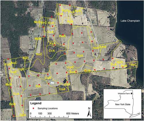
The Cornell University Willsboro Research Farm is a 147-hectare farm located near Lake Champlain with highly variable soils (Entisols, Inceptisols, and Alfisols) formed in glacial deposits (e.g., glacial till, etc.) (Figure 3, Table 2) (Mikhailova et al., 2016). The present study calculates the monetary values of SOC, SIC, and TSC based on soil C data reported by Mikhailova et al. (2016), which is obtained from SSURGO and field measurements. Detailed descriptions of sampling, laboratory analyses, and spatial analyses can be obtained from Mikhailova et al. (2016).

Table 2. Soil types within Willsboro Farm, Willsboro, NY

Soil order/Soil series	Taxonomic class	Map unit symbol	Total area (m^2)
Slight weathering
Entisols			378,691
Claverack loamy fine sand, 3% to 8% slopes	Sandy over clayey, mixed, superactive, nonacid, mesic Aquic Udorthents	CqB	64,230
Cosad loamy fine sand, 0% to 3% slopes	Sandy over clayey, mixed, superactive, nonacid, mesic Aquic Udorthents	CuA	168,530
Deerfield loamy sand, 0% to 3% slopes	Mixed, mesic Aquic Udipsamments	DeA	331
Stafford fine sandy loam, 0% to 3% slopes	Mixed, mesic Typic Psammaquents	StA	145,600
Inceptisols			157,764
Amenia fine sandy loam, 2% to 8% slopes	Coarse-loamy, mixed, active, mesic Aquic Eutrudepts	AmB	3,185
Massena gravelly silt loam, 3% to 8% slopes	Coarse-loamy, mixed, active, nonacid, mesic Aeric Endoaquepts	McB	8,479
Nellis fine sandy loam, 3% to 8% slopes	Coarse-loamy, mixed, superactive, mesic Typic Eutrudepts	NeB	39,030
Nellis fine sandy loam, 8% to 15% slopes	Coarse-loamy, mixed, superactive, mesic Typic Eutrudepts	NeC	107,070
Intermediate weathering
Alfisols			937,940
Bombay gravelly loam, 3% to 8% slopes	Coarse-loamy, mixed, active, mesic Oxyaquic Hapludalfs	BoB	270,615
Churchville loam, 2% to 8% slopes	Fine, illitic, mesic Aeric Endoaqualfs	CpB	36,900
Covington clay, 0% to 3% slopes	Very-fine, mixed, active, mesic Mollic Endoaqualfs	CvA	49,076
Howard gravelly loam, 2% to 8% slopes	Loamy-skeletal, mixed, active, mesic Glossic Hapludalfs	HgB	58,680
Kingsbury silty clay loam, 0% to 3% slopes	Very-fine, mixed, active, mesic Aeric Endoaqualfs	KyA	480,679
Kingsbury silty clay loam, 3% to 8% slopes	Very-fine, mixed, active, mesic Aeric Endoaqualfs	KyB	41,990
Totals			1,474,395

Figure 3. Map of Willsboro Farm, Willsboro, NY (Essex County) with the following soil types: Entisols (Claverack loamy fine sand, 3% to 8% slopes, CqB; Cosad loamy fine sand, 0% to 3% slopes, CuA; Deerfield loamy sand, 0% to 3% slopes, DeA; Stafford fine sandy loam, 0% to 3% slopes, StA), Inceptisols (Amenia fine sandy loam, 2% to 8% slopes, AmB; Massena gravelly silt loam, 3 to 8% slopes, McB; Nellis fine sandy loam, 3% to 8% slopes, NeB; Nellis fine sandy loam, 8% to 15% slopes, NeC), and Alfisols (Bombay gravelly loam, 3% to 8% slopes, BoB; Churchville loam, 2% to 8% slopes, CqB; Covington clay, 0% to 3% slopes, CvA; Howard gravelly loam, 2% to 8% slopes, HgB; Kingsbury silty clay loam, 0% to 3% slopes, KyA; Kingsbury silty clay loam, 3% to 8% slopes, KyB).

2.2. The accounting framework and monetary valuation approach

This study used both biophysical (science-based) and administrative (boundary-based) accounts to calculate monetary values for SOC, SIC, and TSC (Table 3) based on estimated values of SOC, SIC, and TSC storage (in kg) and content (in kg m⁻²) for the Willsboro Farm as reported by Mikhailova et al. (2016). Monetary valuation for SOC, SIC, and TSC storage and content was determined using the concept of avoided costs, in this specific case, the avoided social costs associated with emission of CO₂ to the atmosphere. The EPA has determined the SC-CO2 emissions to be 42 USD per metric ton of CO₂, applicable for the year 2020 based on 2007 U.S. dollars and an average discount rate of 3% (EPA, 2016). According to the EPA, the SC-CO₂ is intended to be a comprehensive estimate of climate change damages, but it can underestimate the true damages and cost of CO₂ emissions due to the exclusion of various important climate change impacts recognized in the literature (EPA, 2016). For the Willsboro Farm, mean storage and content values for SOC, SIC, and TSC by depth, soil order, and soil series were acquired from (Mikhailova et al., 2016, 1996). SOC, SIC, TSC storage and content values were then converted to U.S. dollars and dollars per square meter in Microsoft Excel using the following generalized equations (applied individually to SOC, SIC, TSC), noting that a metric ton is equivalent to 1 megagram (Mg) or 100 kilograms (kg):

(1) $\mathrm{\$}=\left(\mathrm{S}\mathrm{C}\mathrm{S}\mathrm{t}\mathrm{o}\mathrm{r}\mathrm{a}\mathrm{g}\mathrm{e},\mathrm{k}\mathrm{g}\right)\times \frac{1\mathrm{M}\mathrm{g}}{{10}^3\mathrm{k}\mathrm{g}}\times \frac{44\mathrm{M}\mathrm{g}\mathrm{C}{\mathrm{O}}_2}{12\mathrm{M}\mathrm{g}\mathrm{S}\mathrm{C}}\times \frac{\mathrm{\$}42}{\mathrm{M}\mathrm{g}\mathrm{C}{\mathrm{O}}_2}$(1)

(2) $\frac{\mathrm{\$}}{{\mathrm{m}}^2}=\left(\mathrm{S}\mathrm{C}\mathrm{C}\mathrm{o}\mathrm{n}\mathrm{t}\mathrm{e}\mathrm{n}\mathrm{t},\frac{\mathrm{k}\mathrm{g}}{{\mathrm{m}}^2}\right)\times \frac{1\mathrm{M}\mathrm{g}}{{10}^3\mathrm{k}\mathrm{g}}\times \frac{44\mathrm{M}\mathrm{g}\mathrm{C}{\mathrm{O}}_2}{12\mathrm{M}\mathrm{g}\mathrm{S}\mathrm{C}}\times \frac{\mathrm{\$}42}{\mathrm{M}\mathrm{g}\mathrm{C}{\mathrm{O}}_2}$(2)

Table 3. A conceptual overview of the accounting framework used in this study (adapted from Groshans et al., 2019)

Biophysical accounts (Science-based)	Administrative accounts (Boundary-based)	Monetary account(s)	Benefit(s)	Total value
Soil extent:	Administrative extent:	Ecosystem good(s) and service(s):	Sector:	Types of value:
Separate constitute stock 1: Soil organic carbon (SOC)
Separate constitute stock 2: Soil inorganic carbon (SIC)
Composite (total) stock: Total soil carbon (TSC) = SOC + SIC
			Environment:	Social cost of carbon (SC-CO2) and avoided emissions:
- Soil order - Soil series - Soil depth	- Farm - Soil map unit (SMU)	- Regulating (e.g., carbon sequestration)	- Carbon sequestration	- $42 per metric ton of CO2 (2007 U.S. dollars with an average discount rate of 3% (EPA, 2016))

For example, for Alfisols, Mikhailova et al. (2016) reported mean SOC storage and content numbers of 9.76 × 10⁶ kg and 10.4 kg∙m⁻², respectively, based on the SSURGO database. Using these two numbers with a conversion factor for SOC to CO₂ and the EPA dollar value for the SC-CO₂ results in a mean SOC value of about 1.5 million U.S. dollars ($1.5 M) and an area-normalized mean SOC value of about $1.60 m⁻², respectively, for Alfisols.

3. Results

SOC, SIC, and TSC at the Willsboro farm, that either formed naturally (e.g., decomposition of organic matter, etc.), or anthropogenically (e.g., compost additions, liming, etc.) were assigned a monetary value based on the avoided SC-CO₂ from the long-term damage as a result of the emission of a metric ton of carbon dioxide (CO₂). The total calculated monetary value for TSC storage at the Willsboro Farm was about 7.3 million U.S. dollars ($7.3 M) based on the SSURGO data (Table 4), but only about $2.7 M to $2.8 M based on field measurements (Tables 5 and 6). The total calculated monetary value for SOC was similar between SSURGO ($2.5M) and field data ($2.2M) (Figure 4). However, there was a remarkable difference in the total calculated monetary value for SIC: $4.8 M (SSURGO) compared to $0.55 M (field-based estimate) (Figure 4). The estimated values associated with SOC, SIC, and TSC at the Willsboro farm vary by data source (SSURGO versus field-obtained estimates), soil order, and soil map unit (SMU) (Figure 5).

Table 4. Total and area-normalized monetary values of soil organic carbon (SOC), soil inorganic carbon (SIC), and total soil carbon (TSC) storage by soil type and soil order from SSURGO (2015) at the Willsboro Farm (NY), based on a social cost of carbon (SC-CO₂) of $42 per metric ton of CO₂ (EPA, 2016)

		—- Mean SOC—–		——Mean SIC——		—- Mean TSC—-
Soil order/ map unit symbol	Total reported depth (cm)	Total value ($)	Value per area ($ m^−2)	Total value ($)	Value per area ($ m^−2)	Total Value ($)	Value per Area ($ m^−2)
Slight weathering
Entisols (total)	183 ± 0^a	768,460	2.03	523,600	1.38	1,292,060	3.41
CqB	183	106,722	1.66	155,540	2.42	261,800	4.08
CuA	183	338,800	2.01	368,060	2.19	706,860	4.19
DeA	183	650	1.96	0	0	650	1.96
StA	183	321,860	2.21	0	0	321,860	2.21
Inceptisols (total)	183 ± 0	251,020	1.59	562,100	3.57	813,120	5.16
AmB	183	4,528	1.42	14,599	4.59	19,096	6.01
McB	183	21,714	2.56	38,962	4.60	60,676	7.16
NeB	183	60,060	1.54	135,982	3.49	195,580	5.02
NeC	183	164,780	1.54	372,680	3.49	537,460	5.02
Intermediate weathering
Alfisols (total)	201 ± 27	1,503,040	1.60	3,711,400	3.97	5,220,600	5.57
BoB	183	406,560	1.50	896,280	3.31	1,302,840	4.81
CpB	183	63,140	1.71	183,260	4.97	246,400	6.70
CvA	183	146,916	2.99	122,738	2.50	269,500	5.50
HgB	183	55,594	0.95	96,096	1.64	151,844	2.59
KyA	236	763,840	1.59	2,217,600	4.63	2,987,600	6.22
KyB	236	66,682	1.59	194,040	4.63	261,800	6.22
Totals		2,522,520		4,797,100		7,325,780

Note: ^aMean ± standard deviations for the reported depths in the soil order.

Table 5. Total and area-normalized values of soil organic carbon (SOC), soil inorganic carbon (SIC), and total soil carbon (TSC) storage by soil type and soil order from averaged soil core results (original data from Mikhailova et al., 1996) at the Willsboro Farm (NY), based on a social cost of carbon (SC-CO₂) of $42 per metric ton of CO₂ (EPA, 2016)

			——Mean SOC—		——- Mean SIC—–		——Mean TSC—-
Soil order/ map unit symbol	Number of cores	Core depth (cm)	Total value ($)	Value per area ($ m^−2)	Total value ($)	Value per area ($ m^−2)	Total value ($)	Value per area ($ m^−2)
Slight weathering
Entisols (total)	18	84 ± 21^a	531,300	1.40^b	96,250	0.25	626,780	1.66
CqB	4	84 ± 20	114,884	1.79	3,065	0.05	117,964	1.84
CuA	6	83 ± 31	229,460	1.36	90,860	0.54	318,780	1.89
DeA	1	91	691	2.09	0	0	691	2.09
StA	7	85 ± 15	187,880	1.29	2,402	0.02	189,420	1.30
Inceptisols (total)	4	63 ± 33	198,660	1.26	27,720	0.18	226,380	1.43
AmB	n/a^c	n/a	n/a	n/a	n/a	n/a	n/a	n/a
McB	n/a	n/a	n/a	n/a	n/a	n/a	n/a	n/a
NeB	3	74 ± 31	55,440	1.42	25,718	0.66	81,158	2.08
NeC	1	30	128,282	1.20	0	0.00	128,282	1.20
Intermediate weathering
Alfisols (total)	32	84 ± 29	1,516,900	1.62	421,960	0.45	1,940,400	2.07
BoB	10	68 ± 37	269,500	0.99	104,104	0.39	374,220	1.38
CpB	n/a	n/a	n/a	n/a	n/a	n/a	n/a	n/a
CvA	1	92	142,758	2.91	0	0	142,758	2.91
HgB	n/a	n/a	n/a	n/a	n/a	n/a	n/a	n/a
KyA	19	94 ± 19	882,420	1.84	267,960	0.56	1,150,380	2.39
KyB	2	115 ± 5	67,452	1.60	6,175	0.15	73,612	1.75
Totals			2,246,860		545,930		2,793,560

Note: ^aMean ± standard deviations for the reported depths in the soil order. ^bReported value omits areas of SMUs from which no soil cores were taken. ^cn/a: not applicable. No soil core was taken from the specific SMU.

Table 6. Total and area-normalized values of soil organic carbon (SOC), soil inorganic carbon (SIC), and total soil carbon (TSC) storage by soil type and soil order from interpolated soil core results (original data from Mikhailova et al., 1996) at the Willsboro Farm (NY), based on a social cost of carbon (SC-CO₂) of $42 per metric ton of CO₂ (EPA, 2016)

	——Mean SOC—–		——- Mean SIC—–		——Mean TSC—–
Soil order/ map unit symbol	Total value ($)	Value per area ($ m^−2)	Total value ($)	Value per area ($ m^−2)	Total value ($)	Value per Area ($ m^−2)
Slight weathering
Entisols (total)	546,700	1.44	76,230	0.20	622,160	1.64
CqB	108,878	1.69	7,715	0.12	116,424	1.81
CuA	234,080	1.39	61,754	0.37	295,680	1.76
DeA	687	2.07	4	0.01	691	2.09
StA	201,740	1.39	6,730	0.05	209,440	1.43
Inceptisols (total)	209,440	1.33	65,604	0.42	274,120	1.74
AmB	5,544	1.74	2,264	0.71	7,808	2.45
McB	10,734	1.27	1,848	0.22	12,566	1.48
NeB	63,294	1.62	27,258	0.70	90,706	2.32
NeC	129,668	1.21	34,188	0.32	163,240	1.53
Intermediate weathering
Alfisols (total)	1,438,360	1.53	411,180	0.44	1,848,000	1.97
BoB	329,560	1.22	103,334	0.38	432,740	1.60
CpB	65,450	1.77	24,332	0.66	89,474	2.43
CvA	62,986	1.28	35,728	0.73	98,560	2.01
HgB	73,150	1.25	715	0.12	79,926	1.36
KyA	848,540	1.76	231,000	0.48	1,079,540	2.25
KyB	58,520	1.39	8,917	0.21	67,452	1.60
Totals	2,194,500		553,014		2,744,280

Figure 4. Value of total soil carbon (TSC) (based on mean) by different pools (SOC=soil organic carbon, SIC=soil inorganic carbon) at the Willsboro Farm, Willsboro, NY: (a) based on SSURGO database (soil depth range: 183–236cm), (b) based on interpolated field measurements (soil depth range: 30–115cm) based on soil C numbers from Mikhailova et al. (2016) and a SC–CO₂ of $42 per metric ton of CO₂ (EPA, 2016).

3.1. Monetary values of SOC, SIC, and TSC by soil order and SMU (SSURGO)

Monetary values based on SOC storage for the three soil orders were ranked: 1) Alfisols ($1.5M), 2) Entisols ($770,000), and 3) Inceptisols ($250,000) (Table 4). Monetary values based on SOC content for the soil orders, which are equivalent to area-normalized monetary values, were: 1) Entisols ($2.00 m⁻²), and 2) Inceptisols and Alfisols (each at at $1.60 m⁻²). For SIC, the monetary values for the soil orders were ranked: 1) Alfisols ($3.7 M), 2) Inceptisols ($560,000), and 3) Entisols ($520,000) (Table 4) while the area-normalized monetary values for SIC were: 1) Alfisols ($4.00 m⁻²), 2) Inceptisols ($3.60 m⁻²), and 3) Entisols ($1.40 m⁻²). Lastly, the monetary values for TSC storage for the soil orders were ranked: 1) Alfisols ($5.2 M), 2) Entisols ($1.3 M), and 3) Inceptisols ($810,000) (Table 4) while the area-normalized monetary values for TSC were: 1) Alfisols ($5.60 m⁻²), 2) Inceptisols ($5.20 m⁻²), and 3) Entisols ($3.40 m⁻²).

The total monetary value of TSC storage on the Willsboro Farm was $7.3 M based on the SSURGO database. The contribution and distribution of the SOC and SIC reservoirs to the total monetary value were $2.5 M (34%) for SOC storage and $4.8 M (66%) for SIC storage (Figure 4 & Figure 5). For Entisols, the distribution of SOC and SIC was 59% and 41%, respectively, while its corresponding SMU had distributions of SOC = 72 ± 32% and SIC = 28 ± 32%. In contrast, Inceptisols on the Willsboro Farm had an overall distribution of SOC = 29% and SIC = 71% and its corresponding SMUs had distributions of SOC = 30 ± 5% and SIC = 70 ± 5%. Alfisols were similar to Inceptisols, with an overall distribution of SOC = 31% and SIC = 69% while its corresponding SMUs had distributions of SOC = 33 ± 11% and SIC = 67 ± 11%.

3.2. Monetary values of SOC, SIC, and TSC by soil order and SMU (field measurements)

3.2.1. Averaged soil core results

Monetary values based on SOC storage for the three soil orders were ranked: 1) Alfisols ($1.5 M), 2) Entisols ($530,000), and 3) Inceptisols ($200,000) (Table 5) while the area-normalized monetary values for SOC were: 1) Alfisols ($1.60 m⁻²), 2) Entisols ($1.40 m⁻²), and Inceptisols ($1.30 m⁻²). For SIC, the monetary values for the soil orders were ranked: 1) Alfisols ($420,000), 2) Entisols ($96,000), and 3) Inceptisols ($28,000) (Table 5) while the area-normalized monetary values for SIC were: 1) Alfisols ($0.40 m⁻²), 2) Entisols ($0.30 m⁻²), and 3) Inceptisols ($0.20 m⁻²). Lastly, the monetary values for TSC storage for the soil orders were ranked: 1) Alfisols ($1.9 M), 2) Entisols ($630,000), and 3) Inceptisols ($230,000) (Table 5) while the area-normalized monetary values for TSC were: 1) Alfisols ($2.10 m⁻²), 2) Entisols ($1.70 m⁻²), and 3) Inceptisols ($1.40 m⁻²).

The total monetary value of TSC storage on the Willsboro Farm was $2.8 M based on averaging soil core results collected from each SMU. The contribution and distribution of the SOC and SIC reservoirs to the total monetary value were $2.2 M (80%) for SOC storage and $0.55 M (20%) for SIC storage. For Entisols, the distribution of SOC and SIC was 85% and 15%, respectively, while its corresponding SMUs had distributions of SOC = 92 ± 13% and SIC = 8 ± 13%. Inceptisols were similar to Entisols, with an overall distribution of SOC = 88% and SIC = 12% while its corresponding SMUs had distributions of SOC = 84 ± 22% and SIC = 16 ± 22%. Alfisols were less similar, with an overall distribution of SOC = 78% and SIC = 22% while its corresponding SMUs had distributions of SOC = 85 ± 13% and SIC = 15 ± 13%.

3.2.2. Interpolated soil core results

Monetary values based on SOC storage for the three soil orders were ranked: 1) Alfisols ($1.4 M), 2) Entisols ($550,000), and 3) Inceptisols ($210,000) (Table 6) while the area-normalized monetary values for SOC were: 1) Alfisols ($1.50 m⁻²), and 2) Entisols ($1.40 m⁻²), and 3) Inceptisols ($1.30 m⁻²). For SIC, the monetary values for the soil orders were ranked: 1) Alfisols ($410,000), 2) Entisols ($76,000), and 3) Inceptisols ($66,000) (Table 6) while the area-normalized monetary values for SIC were: 1) Alfisols and Inceptisols ($0.40 m⁻²), and 2) Entisols ($0.20 m⁻²). Lastly, the monetary values for TSC storage for the soil orders were ranked: 1) Alfisols ($1.8 M), 2) Entisols ($620,000), and 3) Inceptisols ($270,000) (Table 6) while the area-normalized monetary values for TSC were: 1) Alfisols ($2.00 m⁻²), 2) Inceptisols ($1.70 m⁻²), and 3) Entisols ($1.60 m⁻²).

The total monetary value of TSC storage on the Willsboro Farm was $2.7 M based on inverse distance weighting interpolation of the individual soil cores and then summing the grids contained within each SMU. With this approach, the contribution and distribution of the SOC and SIC reservoirs to the total monetary value were $2.2 M (80%) for SOC storage and $0.55 M (20%) for SIC storage. For Entisols, the distribution of SOC and SIC was 88% and 12%, respectively, while its corresponding SMUs had distributions of SOC = 92 ± 9% and SIC = 8 ± 9%. In contrast, Inceptisols had an overall distribution of SOC = 76% and SIC = 24% while its corresponding SMUs had distributions of SOC = 76 ± 7% and SIC = 24 ± 7%. Alfisols were similar to Inceptisols, with an overall distribution of SOC = 78% and SIC = 22% while its corresponding SMUs had distributions of SOC = 78 ± 10% and SIC = 22 ± 10%.

4. Discussion

Soil is an essential resource for agricultural production with a wide range of uses and users; consequently, agricultural production relies upon the numerous ES provided by soil (e.g., provisioning, regulating, etc.). In a free market system, prices for goods and services provided by soil resources would be self-regulated by the open market and consumers to ensure socially optimal results (Drummond & Goodwin, 2004). Markets, while mostly efficient in dealing with agricultural goods and ES obtained from soil, do not always provide socially optimal results when it comes to environmental problems resulting from agricultural production. For example, agricultural production at a farm-scale (e.g., private ownership) is often accompanied by GHG emissions (e.g., CO₂, etc.) from soil (e.g., private ownership) into the atmosphere (a common-pool resource), therefore generating externalities (external to the market)—social costs for all members of society. In other words, unlike regular agricultural commodities, environmental externalities are generally not “private goods” which can be traded in an open market (Shortle & Uetake, 2015). Instead, they are “public” or “quasi-public” externalities, which can be a source of economic inefficiency and market failure (Landsburg, 2008; Shortle & Uetake, 2015). Carbon dioxide emissions to the atmosphere have both positive and negative externalities: positive—emitted CO₂ is utilized in photosynthesis (biotic) or C sequestration in the form of soil (pedogenic) carbonates (abiotic); negative—excess emitted CO₂ contributes to the build-up of GHG in the atmosphere. Another problem causing market failure is poorly defined property rights. Soil property rights are part of farm ownership, but the property rights for the costs and benefits of CO₂ emissions to the atmosphere are not defined or not clearly defined. It has been reported that 12,000 years of human-induced changes to land cover and land use has resulted in the loss of 133 Pg C from the soil (which may be as much as $20.5 T (T = trillion = 10¹²), based on calculations using eq. 1(1) $\mathrm{\$}=\left(\mathrm{S}\mathrm{C}\mathrm{S}\mathrm{t}\mathrm{o}\mathrm{r}\mathrm{a}\mathrm{g}\mathrm{e},\mathrm{k}\mathrm{g}\right)\times \frac{1\mathrm{M}\mathrm{g}}{{10}^3\mathrm{k}\mathrm{g}}\times \frac{44\mathrm{M}\mathrm{g}\mathrm{C}{\mathrm{O}}_2}{12\mathrm{M}\mathrm{g}\mathrm{S}\mathrm{C}}\times \frac{\mathrm{\$}42}{\mathrm{M}\mathrm{g}\mathrm{C}{\mathrm{O}}_2}$(1) and $42/Mg C) with hotspots of soil C loss, in major cropping and degraded grazing areas (Sanderman et al., 2017).

Sustainable agriculture requires an integration of science-based data with socio-economic data to achieve social profit and cost-effective reductions in GHG emissions (Adewale et al., 2016). For example, Adewale et al. (2016) identified hotspots in the carbon emission footprint of a small-scale organic vegetable farm in Washington State (U.S.), where the carbon emission footprint was attributed to fuel, fertilization, irrigation, and soil CO₂ releases which were assumed to be constant through production and soil type. This type of research, however, did not translate the carbon emission footprint into monetary terms and did not use soil spatial data to incorporate soil C variability and associated hotspot locations in the farm fields.

Digital soil surveys are an important government created resource, which provides information about soil and its properties at various scales, and is often used for management-decisions in a free market system, especially when it comes to provisioning ES supplied by soil. Can data in soil surveys be a useful source of information when dealing with the market failure associated with costs and benefits of CO₂ from soil? It is nearly impossible to measure soil CO₂ emissions on a large scale; however, it is feasible to measure and assess the soil C content over time to understand soil C loss or sequestration (Smith et al., 2019).

In the case of Willsboro Farm, reported soil survey and field values for TSC, SOC, and SIC are based on recent inventories without considering the original losses/gains because of various uses (e.g., agricultural production, etc.) (Sanderman et al., 2017). There is a remarkable difference in values for TSC, SOC, and SIC depending on the source of information: SSURGO versus field data. According to the SSURGO data, the total value of TSC (based on mean) is $7.3 M (with 34% attributed to SOC, and 66% attributed to SIC), which is almost 2.6 times higher than reported field data with the total value of TSC of $2.7 M (with 80% attributed to SOC, and 20% attributed to SIC) (Figure 4). Comparison of SSURGO and field data based on a square meter and SMU also reveal remarkable differences in monetary values (Figure 5). Comparison of mean area-normalized values of SOC, SIC, and TSC storage by soil order from STATSGO, SSURGO, and field sampling also show notable differences in values (Table 7). Although total soil C estimates are important in overall accounting, this analysis shows that from a management point of view some soil orders have higher contribution to the avoided SC-CO₂emissions. For example, Alfisols in the Willsboro farm can contribute more than 70% of the avoided SC-CO₂ emissions, indicating a few “hotspot” areas (Yingjie et al., 2017) with a high potential monetary value as a result of agricultural use. 

Table 7. Comparison of mean area-normalized values of soil organic carbon (SOC), soil inorganic carbon (SIC), and total soil carbon (TSC) storage by soil order from STATSGO (based on numbers from Guo et al., 2006), SSURGO, and field sampling at the Willsboro Farm (NY), based on a social cost of carbon (SC-CO₂) of $42 per metric ton of CO₂ (EPA, 2016)

Soil order, Data source, Scale	Total reported depth (cm)	SOC value per area ($ m^−2)	SIC value per area ($ m^−2)	TSC value per area ($ m^−2)
Slight weathering
Entisols
- STATSGO (NY state)	200	1.23	0.74	1.97
- SSURGO (Farm)	183 ± 0^a	2.03	1.38	3.41
- Field cores (Farm)	84 ± 21	1.40	0.25	1.66
- Interpolated field cores (Farm)	84 ± 21	1.44	0.20	1.64
Inceptisols
- STATSGO (NY state)	200	1.37	0.79	2.16
- SSURGO (Farm)	183 ± 0	1.59	3.57	5.16
- Field cores (Farm)	63 ± 33	1.26	0.18	1.43
- Interpolated field cores (Farm)	63 ± 33	1.33	0.42	1.74
Intermediate weathering
Alfisols
- STATSGO (NY state)	200	1.16	0.66	1.82
- SSURGO (Farm)	201 ± 27	1.60	3.97	5.57
- Field cores (Farm)	84 ± 29	1.62	0.45	2.07
- Interpolated field cores (Farm)	84 ± 29	1.53	0.44	1.97

Note: ^aMean ± standard deviations for the reported depths in the soil order.

Figure 5. Value of total soil carbon (TSC) (based on mean) based on a SC-CO₂ of $42/metric ton of CO₂ at the Willsboro Farm, Willsboro, NY: (a) based on SSURGO database (soil depth range: 183–236 cm), (b) based on averaged field measurements (soil depth range: 30–115 cm).

According to Drummond and Goodwin (2004), “appropriate government intervention to correct market failure requires accurate information about the market failure itself and about what is socially optimal. If information is inadequate or incorrect, then intervention may be worse than the market itself.” Freely available soil surveys contain data for SOC, SIC, and TSC (which can be calculated through summation of SOC and SIC), however, this information can be inaccurate at the farm scale based on earlier research (Mikhailova et al., 2016) leading to inaccurate monetary estimates of the avoided SC-CO₂ emissions. There are several sources of these inaccuracies: depth of sampling, the density of sampling, different laboratory and field methods of C measurement, method of reporting, differences in data interpolation techniques, its static nature, and other reasons (Indorante et al., 1996).

Despite these limitations, soil survey information is often the only comprehensive soil information typically available and may be more accurate at different spatial scales. It is important to note that soil survey information intended to “describe the characteristics of the soils in a given area, classify the soils according to a standard system of classification, plot the boundaries of the soils on a map, and make predictions about the behavior of soils (Soil Science Division Staff, 2017).” The major advantage of soil survey maps is the “they portray the spatial distribution of stable, recognizable and repeating patters of soils that usually occupy identifiable portions of the landscape (Hengl & MacMillan, 2019).” Science-based soil ES valuations depend on these soil–landscape relationships (Eastburn et al., 2017). Recent digital upgrades to soil survey (e.g., Web Soil Survey) made it user-friendly and accessible to a wide range of audiences (e.g., educators, students, etc.).

Current digital soil surveys in the U.S. include the following typical information, which can be used for the soil carbon ES assessment at various scales (Chandler et al., 2018; Soil Survey Staff, 2020):

• “A general soil map with a brief description of each of the major soil types found in the county along with their characteristics.

• Detailed aerial photographs with specific soil types outlined and indexed.

• Tables containing general information about the various soils such as total area, comparisons of production of typical crops, and common range plants.

• Tables containing specific physical, chemical, and engineering properties including data on SOC and SIC, which can be used to calculate TSC by summation.”

• Soil C data can be also displayed in the map format with a table summary underneath, which explains the benefits of SOC and SIC in agricultural production. This summary can be supplemented with an explanation about corresponding social costs associated with using soil C (e.g., avoided social costs of carbon emissions, SC-CO₂ etc.).

Based on this information, the property boundaries can be outlined using area of interest (AOI) tool, soil types can be mapped, SOC, SIC data can be downloaded in the table format, and SC-CO₂ can be estimated for the total areas of the soil types and on an area basis. This information can be useful in planning, cost-benefit analysis, identifying hotspots (based on SMU boundaries) associated with high avoided SC-CO₂ emissions from soil (Figures 6–8). It can be also used for educational purposes as well as a warning about unsustainable use of soil C resources and adverse impacts to the environment. According to Burkhard and Maes (2017), costs and benefits of agricultural production based on ES very often exceed spatial boundaries of an individual farm. The challenge of balancing the costs and benefits of soil C management is further complicated by policy and economic challenges considering complex tapestry of farms and soil types within them (Alexander et al., 2015; Amundson & Biadeau, 2018).

Figure 6. Value of soil organic carbon (SOC) based on a SC-CO₂ of $42/metric ton of CO₂ at the Willsboro Farm, Willsboro, NY: (a) from SSURGO results averaged over SMUs, (b) interpolated from soil core sample results.

Figure 7. Value of soil inorganic carbon (SIC) based on a SC-CO₂ of $42/metric ton of CO₂ at the Willsboro Farm, Willsboro, NY: (a) from SSURGO results averaged over soil map units (SMUs), (b) interpolated from soil core sample results.

Figure 8. Value of total soil carbon (TSC) based on a SC-CO₂ of $42/metric ton of CO₂ at the Willsboro Farm, Willsboro, NY: (a) from SSURGO results averaged over soil map units (SMUs), (b) interpolated from soil core sample results.

This study demonstrated that monetary valuations using SSURGO data represent a uniform soil C distribution throughout a map unit and do not represent the actual hotspots seen in interpolated field data maps at the field and farm scales (Table 8). At the same time, field interpolated monetary values of social costs of C are not as useful by themselves unless they are put in the context of soil survey information (e.g., SMU boundaries, soil taxonomic information, etc.).

Table 8. The proportion of the area occupied by different management zones according to the SSURGO database, and field data based on interpolation of soil core sample results for soil organic carbon (SOC), soil inorganic carbon (SIC), and total soil carbon (TSC)

Management zones
Soil carbon classes ($ m^−2)	Area (m^2)	Area (%)
SOC: SSURGO database
0–0.55	0	0
0.55–1.10	58,681	3.98
1.10–1.65	942,583	63.93
1.65–2.20	269,962	18.31
2.20–2.75	154,075	10.45
2.75–3.30	49,097	3.33
SOC: Interpolated from field soil core sample results
0–0.55	7,519	0.51
0.55–1.10	256,103	17.37
1.10–1.65	738,968	50.12
1.65–2.20	415,043	28.15
2.20–2.75	51,015	3.46
2.75–3.30	5,750	0.39
SIC: SSURGO database
0–0.85	145,818	9.89
0.85–1.70	58,681	3.98
1.70–2.55	552,752	37.49
2.55–3.40	0.00	0.00
3.40–4.25	145,965	9.90
4.25–5.10	571,182	38.74
SIC: Interpolated from field soil core sample results
0–0.40	1,005,834	68.22
0.40–0.80	306,380	20.78
0.80–1.20	103,355	7.01
1.20–1.60	38,039	2.58
1.60–2.00	18,872	1.28
2.00–2.40	1,917	0.13
TSC: SSURGO database
0–1.2	0	0
1.2–2.4	145,965	9.90
2.4–3.6	58,534	3.97
3.6–4.8	232,807	15.79
4.8–6.0	465,910	31.60
6.0–7.2	571,182	38.74
TSC: Interpolated from field soil core sample results
0–1.2	105,272	7.14
1.2–2.4	1,134,254	76.93
2.4–3.6	228,532	15.50
3.6–4.8	6.340	0.43

5. Conclusions

Agriculture utilizes various ES provided by soil resources at the farm, which results in benefits (e.g., crop production, etc.) and costs (social costs of carbon, SC-CO₂) to the human society. Previous efforts to enhance sustainability through precision agriculture management have not considered the social costs of CO₂ emissions from soil. Expressing and mapping soil C in terms of avoided SC-CO₂ emissions converts soil carbon data to economic terms defined by humans which can be combined with other methods of cost-benefit analysis used in agriculture. This study analyzed differences in monetary values at the farm scale using the SSURGO database and detailed field measurements. SSURGO-derived avoided social costs of TSC emissions were higher than the farm-specific field measurements by almost 2.6 times. These differences in values can be attributed to the limitations of the soil survey information (e.g., soil C values measured in a pedon from a “type location,” the extrapolated-with-depth soil C data, etc.). Regardless of the differences in magnitude of monetary values, the trends were similar for both SSURGO and field methods with Alfisols having the highest mean total and area-normalized values for SOC, SIC, and TSC. Valuations using SSURGO data represent a uniform soil C distribution throughout a map unit and do not represent the actual hotspots seen in interpolated field data maps at the field and farm scales. Although SSURGO may be useful to identify SCHs at county, state, and regional levels, field data are better suited to identify SCHs at the farm- and field-scales. Compared to SSURGO data, field data provided a greater detail in identifying and delineating SCHs within the farm. Proposed SCHs concept and methodology can be applied to the farms with different types of soil carbon due to geographic differences in soil carbon distribution in the country. It can be also incorporated with precision agriculture techniques (e.g., recording, etc.) and Farm Management Information System (FMIS) to enhance a decision support system to ensure both profitability and sustainability of agricultural production.

correction

This article has been republished with minor changes. These changes do not impact the academic content of the article.

Disclosure statement

No potential conflict of interest was reported by the authors.

Additional information

Funding

The authors received no direct funding for this research.

Notes on contributors

Elena A. Mikhailova

Elena A. Mikhailova is a professor of Soil Science at Clemson University, SC, USA. Dr. Christopher Post is a professor of Environmental Information Science at Clemson University, SC, USA. Dr. Mark Schlautman is a professor of Environmental Engineering and Earth Sciences at Clemson University, SC, USA. Gregory Post is an undergraduate student in Environmental Studies-Economics at Reed College, OR, USA. Dr. Hamdi Zurqani is a GIS and Remote Sensing research associate in the South Carolina Water Resources Center, SC, USA.

References

- Adewale, C., Higgins, S., Granatstein, D., Stöckle, C. O., Carlson, B. R., Zaher, U. E., & Carpenter-Boggs, L. (2016). Identifying hotspots in the carbon footprint of a small scale organic vegetable farm. Agricultural Systems, 149, 112–19. https://doi.org/10.1016/j.agsy.2016.09.004
- Alexander, P., Paustian, K., Smith, P., & Moran, D. (2015). The economics of soil C sequestration and agricultural emissions abatement. Soil, 1(1), 331–339. https://doi.org/10.5194/soil-1-331-2015
- Amundson, R., & Biadeau, L. (2018). Soil carbon sequestration is an elusive climate mitigation too. Proceedings of the National Academy of Sciences, 115(46), 11652–11656. https://doi.org/10.1073/pnas.1815901115
- Bétard, F., & Peulvast, J. (2019). Geodiversity hotspots: Concept, method and cartographic application for geoconservation purposes at a regional scale. Environmental Management, 63(6), 822–834. https://doi.org/10.1007/s00267-019-01168-5
- Bhattacharyya, T., Chandran, P., Ray, S. K., Mandal, C., Tiwary, P., Pal, D. K., Wani, S. P., & Sahrawat, K. L. (2014). Processes determining the sequestration and maintenance of carbon in soils: A synthesis of research from tropical India. Soil Horizons, 55(4). https://doi.org/10.2136/sh14-01-0001
- Burkhard, B., & Maes, J. (2017). Mapping ecosystem services. Pensoft Publishers.
- Chandler, R. D., Mikhailova, E. A., Post, C. J., Moysey, S. M. J., Schlautman, M. A., Sharp, J. L., & Motallebi, M. (2018). Integrating soil analyses with frameworks for ecosystem services and organizational hierarchy of soil systems. Communications in Soil Science and Plant Analysis, 49(15), 1835–1843. https://doi.org/10.1080/00103624.2018.1474919
- Drummond, H. E., & Goodwin, J. W. (2004). Agricultural economics (Second ed.). Prentice Hall.
- Eastburn, D. J., O’Green, A. T., Tate, K. W., & Roche, L. M. (2017). Multiple ecosystem services in a working landscape. PLoS ONE, 12(3), e0166595. https://doi.org/10.1371/journal.pone.0166595
- EPA. (2016). The social cost of carbon. EPA Fact Sheet. Retrieved March 15, 2019, from. https://19january2017snapshot.epa.gov/climatechange/social-cost-carbon_.html
- Franzluebbers, A. J., Follett, R. F., Johnson, J. M. F., Liebig, M. A., Gregorich, E. G., Parkin, T. B., Smith, J. L., Del Grosso, S. J., Jawson, M. D., & Martens, D. A. (2006). Agricultural exhaust: A reason to invest in soil. Journal of Soil Water Conservation, 61(3), 98A–101A.
- Groshans, G. R., Mikhailova, E. A., Post, C. J., Schlautman, M. A., Cope, M. P., & Zhang, L. (2019). Ecosystem services assessment and valuation of atmospheric magnesium deposition. Geosciences, 9(8), 331. https://doi.org/10.3390/geosciences9080331
- Guo, Y., Amundson, R., Gong, P., & Yu, Q. (2006). Quantity and spatial variability of soil carbon in the conterminous United States. Soil Science Society of America Journal, 70(2), 590–600. https://doi.org/10.2136/sssaj2005.0162
- Harms, T. K., & Grimm, N. B. (2008). Hot spots and hot moments of carbon and nitrogen dynamics in a semiarid riparian zone. Journal of Geophysical Research, 113(G1), G01020. https://doi.org/10.1029/2007JG000588
- Hengl, T., & MacMillan, R. A. (2019). Predictive soil mapping with R. OpenGeoHub foundation. www.soilmapper.org
- Indorante, S. J., McLeese, R. L., Hammer, R. D., Thompson, B. W., & Alexander, D. L. (1996). Positioning soil survey for the 21st century. Journal of Soil and Water Conservation, 51(1), 21–28.
- Johnson, D. W., Miller, W. W., Rau, B. M., & Meadows, M. W. (2011). The natural and potential causes of nutrient hotspots in a Sierra Nevada forest soil. Soil Science, 176(11), 596–610. https://doi.org/10.1097/SS.0b013e31823120a2
- Keestra, S. D., Bouma, J., Wallinga, J., Tittonell, P., Smith, P., Cerda, A., Montanarella, L., Quinton, J. N., Pachepsky, Y., Van der Putten, W. H., Bardgett, R. D., Moolenaar, S., Mol, G., Jansen, B., & Fresco, L. O. (2016). The significance of soils and soil science towards realization of the United Nations Sustainable Development Goals. Soil, 2(2), 111–128. https://doi.org/10.5194/soil-2-111-2016
- Kuzyakov, Y., & Blagodatskaya, E. (2015). Microbial hotspots and hot moments in soil: Concept & review. Soil Biology & Biochemistry, 83, 184–199. https://doi.org/10.1016/j.soilbio.2015.01.025
- Landsburg, S. E. (2008). Price Theory and Applications (7th ed. Thomson Higher Education.
- Mikhailova, E. A., Altememe, A. H., Bawazir, A. A., Chandler, R. D., Cope, M. P., Post, C. J., Stigtlitz, R. Y., Zurqani, H. A., & Schlautman, M. A. (2016). Comparing soil carbon estimates in glaciated soils at a farm scale using geospatial analysis of field and SSURGO data. Geoderma, 281, 119–126. https://doi.org/10.1016/j.geoderma.2016.06.029
- Mikhailova, E. A., Groshans, G. R., Post, C. J., Schlautman, M. A., & Post, G. C. (2019a). Valuation of soil organic carbon stocks in the contiguous United States based on the avoided social cost of carbon emissions. Resources, 8(3), 153. https://doi.org/10.3390/resources8030153
- Mikhailova, E. A., Groshans, G. R., Post, C. J., Schlautman, M. A., & Post, G. C. (2019b). Valuation of total soil carbon stocks in the contiguous United States based on the avoided social cost of carbon emissions. Resources, 8(4), 157. https://doi.org/10.3390/resources8040157
- Mikhailova, E. A., Van Es, H. M., Lucey, R. F., DeGloria, S. D., Schwager, S. J., & Post, C. J. (1996). Soil characterization data for selected pedons from the Willsboro Farm, Essex County. Research Series R96-5. Department of Soil, Crop, and Atmospheric Sciences, Cornell University.
- Sanderman, J., Hengl, T., & Fiske, G. J. (2017). Soil carbon debt of 12,000 years of human land use. Proceedings of the National Academy of Sciences, 114(36), 9575–9580. https://doi.org/10.1073/pnas.1706103114
- Shortle, J., & Uetake, T. (2015). Public goods and externalities: Agri-environmental policy measures in the United States. OECD Food, Agriculture and Fisheries Papers, OECD Publishing.
- Smith, P., Soussana, J., Angers, D., Schipper, L., Chenu, C., Rasse, D. P., Batjes, N. H., van Egmond, F., McNeill, S., Kuhnert, M., Arias-Navarro, C., Olesen, J. E., Chirinda, N., Fornara, D., Wollenberg, E., Álvaro-Fuentes, J., Sanz-Cobena, A., & Klumpp, K. (2019). How to measure, report and verify soil carbon change to realize the potential of soil carbon sequestration for atmospheric greenhouse gas removal. Global Change Biology, 26(1), 219–241. https://doi.org/10.1111/gcb.14815
- Soil Science Division Staff. (2017). Soil Survey Manual. In C. Ditzler, K. Scheffe, & H. C. Monger (Eds.), USDA Handbook 18. Government Printing Office.
- Soil Survey Staff. (2020). Natural Resources Conservation Service, United States Department of Agriculture. Web soil survey. Rretrieved January 24, 2020, from. https://websoilsurvey.sc.egov.usda.gov/
- Tegtmeier, E. M., & Duffy, M. D. (2004). External costs of agricultural production in the United States. International Journal of Agricultural Sustainability, 2(1), 1–20. https://doi.org/10.1080/14735903.2004.9684563
- Tugel, A. J., Herrick, J. E., Brown, J. R., Mausbach, M. J., Puckett, W., & Hipple, K. (2005). Soil change, soil survey, and natural resources decision making: A blueprint for action. Soil Science Society of America Journal, 69(3), 738–747. https://doi.org/10.2136/sssaj2004.0163
- Van Evert, F. K., Gaitán-Cremaschi, D., Fountas, S., & Kempenaar, C. (2017). Can precision agriculture increase the profitability and sustainability of the production of potatoes and olives? Sustainability, 9(10), 1863. https://doi.org/10.3390/su9101863
- Wang, P., Deng, X., Zhou, H., & Yu, S. (2019). Estimates of the social cost of carbon: A review based on meta-analysis. Journal of Cleaner Production, 209, 1494–1507. https://doi.org/10.1016/j.jclepro.2018.11.058
- Yingjie, L., Liwei, Z., Junping, Y., Pengtao, W., Ningke, H., Wei, C., & Bojie, F. (2017). Mapping the hotspots and coldspots of ecosystem services in conservation priority setting. Journal of Geographical Sciences, 27(6), 681–696. https://doi.org/10.1007/s11442-017-1400-x