Manufacturer-retailer inventory model for deteriorating items with price-sensitive credit-linked demand under two-level trade credit financing and profit sharing contract

Abstract

A supply chain of single manufacturer and single retailer is analyzed when units in warehouse are subject to deterioration at a constant rate. The demand is a decreasing function of selling price and increasing function of credit period offered by the retailer to the customers. Manufacturer follows a lot-for-lot production strategy. The manufacturer ensures delay payment to the retailer with agreement that the retailer will share a fraction of the profit realized during the credit period. The total joint profit of the supply chain is maximized with respect to replenishment time, selling price, and credit period. An algorithm is described to find the best strategy. Numerical examples are given to validate the proposed problem. Sensitivity analysis is carried out to examine important model parameters.

Keywords:

• Single manufacturer and single retailer
• deterioration
• lot-for-lot production strategy
• two-level trade credit financing
• price-sensitive credit-linked demand
• profit sharing contract

Public Interest Statement

The proposed problem is interesting for the players working in a supply chain by sharing their interest, information of the product, investment, and also constraints. The decision is critical when manufacturer is using lot-for-lot production strategy to reduce the loss in terms of deterioration of the products. The manufacturer can push his demand by offering promotional tool of credit period to settle the account and also profit sharing. An algorithm is described to find the best strategy. The model can be used by business firm by deploying changes as per their firm policy.

1. Introduction

The fact that the retailer must follow cash-on-delivery strategy is no more advocated in the business transactions. The manufacturer offers retailer a fixed credit period to boost the demand, and decrease his holding and deterioration cost. During this credit period, the retailers sell the items and earn interest on the generated revenue. The manufacturer charges interest on the unsold stock if the account is not settled during allowable credit period. This concept was first formulated by Goyal (1985). Refer to review articles by Chang, Teng, and Goyal (2008) and Shah, Soni, and Jaggi (2010) for available literatures on inventory modeling and trade credit. Giri and Maiti (2013) formulated model which considers that the retailer borrows loan from bank to settle the accounts and concluded that it is advantageous to do payment at the end of the allowable credit period. This offer entices to order more frequently which reduces manufacturer’s inventory. On the other end, it increases holding cost, ordering cost, and deterioration cost if the retailer stocks more items which are deteriorating in nature. So the pay-off is needed between costs of two players.

Most of the citations in review articles are assuming that only supplier is offering a fixed credit period to the retailer. However, if the same intensive is extended to the customer by the retailer, the demand will escalate. Huang (2003) developed an EOQ model in which the supplier offers the retailer a credit period (upstream credit period), and retailer in turn provides a credit period (downstream credit period) to the customer. Huang (2006) formulated an inventory model under two-level trade credit with constrained floor space. Huang (2007) incorporated finite production capacity of the manufacture. Some more related articles are by Huang (2008), Jaggi, Goyal, and Goel (2008), Liao (2008), Shah, Soni, and Shah (2009), Teng, Chang, Chern, and Chan (2007), Teng and Goyal (2007), and their references.

Now-a-days, the researchers are analyzing integrated inventory models with trade credit financing as a promotional tool. Abad and Jaggi (2003) formulated a supplier–buyer inventory model under permissible delay in payments with price-sensitive demand. Sheen and Tsao (2007) discussed a vendor–buyer inventory model with trade credit and quantity discounts for freight cost. Sarmah, Acharya, and Goyal (2007) studied coordination and profit sharing between two players under permissible delay in payments. He and Huang (2013) developed inventory model for two players of a supply chain for non-instantaneous deterioration items where demand is a function of downstream credit-linked demand. Chung and Cárdenas-Barrón (2013) formulated simplified procedure when demand is stock-dependent and two-level trade credit is offered. Jiang, Skouri, Teng, and Ouyang (2014) gave a note on optimal replenishment policies for non-instantaneous deteriorating items with price and stock sensitive demand under permissible delay in payment. Aggarwal and Tyagi analyzed inventory and credit policies with date-terms credit-linked demand in a supply chain. Chung, Cárdenas-Barrón, and Ting (2014) developed an inventory model with non-instantaneous receipt and exponentially deteriorating items for an integrated three layer supply chain system under two levels of trade credit when demand is constant. Chen, Teng, and Skouri (2014) derived economic production quantity model for deteriorating items with up-stream full trade credit and down-stream partial trade credit when production is finite. Feng, Moon, and Ryu (2014) considered revenue-sharing contracts in a supply chain with reliability considerations. Jiang, Ouyang, Cardenas-Barron, and Goyal (2014) computed optimal credit period and purchase units for fixed life time deterioration of items under two-level trade credit scenario. Integrated vendor–buyer models are studied by Chen, Chen, Chiu, Choi, and Sethi (2010), Chen and Kang (2007), Chen and Kang (2010a, 2010b), Chiu, Choi, and Li (2009), Chiu, Choi, and Tang (2011), Ho, Ouyang, and Su (2008), Huang, Tsai, Wu, and Chung (2010), Jaber and Osman (2006), Kim, Hong, and Kim (2011), Ouyang, Ho, and Su (2008), Teng, Chang, and Chem (2012), Yen, Chung, and Chen (2012).

In this paper, we study the impact of two-level trade credit policy on a supply chain comprising of a single-manufacturer and single-retailer. The items in inventory system of both the players are subject to deterioration at a constant rate. The demand is considered to be increasing function of credit period which retailer offers to customer and decreasing function of selling price. It is assumed that the manufacturer offers a fixed credit period to the retailer with the contract that the retailer must share his profit during allowable credit period (Giri & Maiti, 2013). The manufacturer follows a lot-for-lot production policy. The joint profit of the supply chain is maximized with respect to replenishment time, selling price, and credit period to be offered to the customer by the retailer. Solution procedure is outlined to arrive at the best possible solution. Numerical examples are given to support the theoretical developments. The sensitivity of the optimal results with the model parameters is carried out to deduce managerial insights.

2. Notations and assumptions

The proposed problem is formulated with following notations and assumptions.

2.1. Notations

Inventory parameters for manufacturer
Am	=	Setup cost per setup
hm	=	Inventory holding cost per unit per annum
Cm	=	Purchase cost of an item per unit
P	=	Constant production rate
Tm	=	Time delay at which manufacturer starts production
M	=	Fixed credit period (in years) offered by the manufacturer to the retailer
Ilm	=	Loss of interest incurred due to offer of credit period
δ	=	Fraction of profit share by the manufacturer from the retailer during the credit period M; 0 < δ < 1
πm	=	Profit per unit time of a manufacturer

Inventory parameters for retailer
Ar	=	Ordering cost per order
hr	=	Inventory holding cost per unit per annum
Cr	=	Purchase cost of an item per unit
p	=	Selling price per unit (a decision variable)
Ib	=	Interest rate on the loan borrowed from the bank
Ie	=	Interest earned per unit per annum
τ	=	Fraction of customers allowed by the retailer to avail of credit period N; 0 ≤ τ ≤ 1
θ	=	Deterioration rate of items in warehouse; 0 ≤ θ < 1
R(p, N)	=	Retailer’s demand rate (say); R(p, N) = α – ηp + βN; α > 0 denotes scale demand, η > 0 denotes price elasticity markup and β > 0 denotes trade credit markup. (p and N are decision variables)
T	=	Replenishment time (a decision variable)
πr	=	Profit per unit time of a retailer

Relation between inventory parameters

$I_b>I_e,N\le M$

p > C_r > C_m

$T_m=\mathit{\lambda }T,0<\mathit{\lambda }<1$

Objective

Total joint profit per unit time of the supply chain

$\begin{array}{c}\text{Maximize}\mathit{\pi }={\mathit{\pi }}_m+{\mathit{\pi }}_r\hfill \\ \text{subject to}N,p,T\ge 0\hfill \end{array}$

2.2. Assumptions

1. A supply chain of single-manufacturer, single-retailer, and single-item is under consideration.

2. The demand rate R(p, N) for retailer is increasing function of credit period; N offered to customer and decreasing function of selling price; p. The function form of demand rate is R(p, N) = α − ηp + βN. R(p, N) and R are interchangeable.

3. The constant production rate $P(>R)$ to avoid shortages.

4. Replenishment is instantaneous.

5. The planning horizon is infinite to ensure long-term relationships.

6. The manufacturer offers a delay period M to settle the accounts to the retailer with the contract that the retailer will share fraction of his profit incurred during the credit period M. The retailer takes a loan from a bank at the rate I_b to settle the accounts with manufacturer for the purchases made at the end of time M. The loan is repaid to the bank at the end of the cycle time.

7. By offering credit period, the manufacturer incurs interest loss at the rate I_lm per unit per annum.

8. The items in warehouse deteriorate at a constant rate, θ, (0 ≤ θ < 1). The deteriorated units can neither be repaired nor replaced during the cycle time.

3. Mathematical model

3.1. Model for retailer’s inventory system

The retailer’s inventory depletes due to credit-linked price-sensitive demand and deterioration of items in the warehouse. The rate of depletion of inventory at any instant of time $t\in \left[0,T\right]$ is given by the differential equation

$\frac{d{I}_r(t)}{dt}=-R-\mathit{\theta }{I}_r(t),0\le t\le T$ with I_r(T) = 0.

The solution of differential equation is $I_r(t)=\frac{R}{\mathit{\theta }}\left(exp(\mathit{\theta }(T-t))-1\right),0\le t\le T$. The retailer’s cycle starts with $Q=I_r(0)=\frac{R}{\mathit{\theta }}\left(exp(\mathit{\theta }T)-1\right)$ units in warehouse. The basic costs of the retailer are

• Purchase cost of procuring Q units per unit time is $P{C}_r=\frac{C_{r}R}{\mathit{\theta }T}\left(exp(\mathit{\theta }T)-1\right)$.

• Ordering cost per order is $O{C}_r=\frac{A_r}{T}$.

• Holding cost per unit time is $H{C}_r=\frac{h_r}{T}{\int }_0^T{I}_r(t)dt=\frac{h_{r}R}{{\mathit{\theta }}^{2}T}\left(exp(\mathit{\theta }T)-\mathit{\theta }T-1\right)$.

Depending upon the lengths of credit periods M and N offered by the manufacturer and the retailer, respectively, and the cycle time T, following three cases are to be analyzed. Viz. (i) N ≤ M ≤ T, (ii) N ≤ T ≤ M, and (iii) T ≤ N ≤ M. Next, we detail out each case.

Case (i):N ≤ M ≤ T

Here, retailer generates revenue, $S{R}_r=\frac{p}{T}{\int }_0^{T}Rdt$. During [0, M], as per the contractual memorandum, the retailer gives δ% of profit to the manufacturer. So fraction of profit shared is, $F{P}_1=\frac{\mathit{\delta }(p-C_r)RM}{T}$ and the remaining can be used to settle the account. To settle full account at M, the retailer takes a loan from the bank at the rate I_b per unit per annum and repays it at the end of cycle time T. So, the net interest charged by the bank per unit time is $IC{B}_r=\frac{I_b}{T}\left[C_{r}RT-pRM+\mathit{\delta }(p-Cr)MR\right](T-M)$ and interest earned by the retailer during the cycle time T per unit time is $I{E}_{r1}=\frac{P{I}_e}{T}\left[{\int }_0^{M}Rtdt+{\int }_0^{T-M}Rtdt\right]$. Due to offer of trade credit to the customer, the retailer incurs opportunity loss as $O{L}_{r1}=\frac{\mathit{\tau }p{I}_e}{T}{\int }_0^{N}Rtdt$. Hence, retailer’s net profit, π_r1 per unit time is(1) $${\mathit{\pi }}_{r1}(N,p,T)=S{R}_r-P{C}_r-F{P}_1-O{C}_r-H{C}_r-IC{B}_r-O{L}_{r1}+I{E}_{r1}$$(1)

Case (ii):N ≤ T ≤ M

The profit to be shared is, FP₂ = δ(p − C_r)R and the interest earned by the retailer during the cycle time T per unit time is $I{E}_{r2}=\frac{P{I}_e}{T}\left[{\int }_0^{T}Rtdt+Q(M-T)\right]$. Due to offer of trade credit to the customer, the retailer incurs opportunity loss as $O{L}_{r2}=\frac{\mathit{\tau }p{I}_e}{T}{\int }_0^{N}Rtdt$. Here, the retailer has sufficient amount to pay for the purchases so retailer does not borrow any loan. Hence, retailer’s net profit, π_r2 per unit time is(2) $${\mathit{\pi }}_{r2}(N,p,T)=S{R}_r-P{C}_r-F{P}_2-O{C}_r-H{C}_r-O{L}_{r2}+I{E}_{r2}$$(2)

Case (iii):T ≤ N ≤ M

The profit to be shared is, FP₃ = δ(p − C_r)R and the interest earned by the retailer during the cycle time T per unit time is $I{E}_{r3}=\frac{P{I}_e}{T}\left[{\int }_0^{T}Rtdt+Q(M-T)\right]$. Due to offer of trade credit to the customer, the retailer incurs opportunity loss as $O{L}_{r3}=\frac{\mathit{\tau }p{I}_e}{T}\left[{\int }_0^{N}Rtdt+Q(N-T)\right]$. Since, the cycle time ends before the credit period, the retailer does not have to pay interest charges and interest loss due to profit sharing with the manufacturer is zero. Hence, retailer’s net profit, π_r3 per unit time is(3) $${\mathit{\pi }}_{r3}(N,p,T)=S{R}_r-P{C}_r-F{P}_3-O{C}_r-H{C}_r-O{L}_{r3}+I{E}_{r3}$$(3)

3.2. Model for manufacturer’s inventory system

The rate of change of inventory in manufacturer’s warehouse at any instant of time $t\in \left[0,T\right]$ is given by the differential equation $\frac{d{I}_m(t)}{dt}=P-\mathit{\theta }{I}_m(t),t_m\le t\le T$ with I_m(T) = 0.

The solution of differential equation is $I_m(t)=\frac{P}{\mathit{\theta }}\left(1-exp(-\mathit{\theta }(t-t_m))\right),0\le t\le T$. Therefore, holding cost per unit time is $H{C}_m=\frac{h_m}{T}{\int }_{T_m}^T{I}_m(t)dt$ and interest loss occurred per unit time due to allowable credit period M to the retailer is $O{L}_m=\frac{C_{r}P{I}_{lm}(T-T_m)M}{T}$. The setup cost per unit time is $O{C}_m=\frac{A_m}{T}$. Under contract, manufacturer receives δ% of profit earned by the retailer during the credit period. So, fraction of profit gained by the manufacturer per unit time is$$F{P}_m=\left\{\begin{array}{c}F{P}_{m1}=\frac{\mathit{\delta }(p-C_r)RM}{T},M\le T\hfill \\ F{P}_{m2}=\mathit{\delta }(p-C_r)RM>T\hfill \end{array}\right.$$

Hence, the manufacturer’s net profit per unit time is(4) $${\mathit{\pi }}_{m1}(T)=(C_r-C_m)R-O{C}_m-H{C}_m-O{L}_m+F{P}_{m1},M\le T$$(4) (5) $${\mathit{\pi }}_{m2}(T)=(C_r-C_m)R-O{C}_m-H{C}_m-O{L}_m+F{P}_{m2},M>T$$(5)

3.3. Joint profit of the supply chain

The objective of this study is to maximize the profit of supply chain comprising of single-manufacturer and single-retailer. The joint profit of the integrated supply chain is:(6) $$\mathit{\pi }(N,p,T)=\left\{\begin{array}{c}{\mathit{\pi }}_1(N,p,T)={\mathit{\pi }}_{r1}(N,p,T)+{\mathit{\pi }}_{m1}(T),N\le M\le T\hfill \\ {\mathit{\pi }}_2(N,p,T)={\mathit{\pi }}_{r2}(N,p,T)+{\mathit{\pi }}_{m2}(T),N\le T\le M\hfill \\ {\mathit{\pi }}_3(N,p,T)={\mathit{\pi }}_{r3}(N,p,T)+{\mathit{\pi }}_{m2}(T),T\le N\le M\hfill \end{array}\right.$$(6)

For given values of p and N, we have π₁(M/p, N) = π₂(M/p, N) and π₂(N/p, N) = π₃(N/p, N). Thus, π_i, i = 1, 2, 3 are well-defined functions of three decision variables. Next, we outline steps to find the best solution for the supply chain.

Algorithm

Step 1: Set numerical values for the inventory parameters.

Step 2: Set $\frac{\mathit{\partial }{\mathit{\pi }}_i}{\mathit{\partial }N}=0,\frac{\mathit{\partial }{\mathit{\pi }}_i}{\mathit{\partial }p}=0\text{and}\frac{\mathit{\partial }{\mathit{\pi }}_i}{\mathit{\partial }T}=0,i=1,2,3$ and solve by Maple 14 simultaneously for N, p and T. Find out the appropriate scenario and for that obtained joint profit.

Step 3: Check sufficiency condition graphically.

4. Numerical examples

Example 1: Consider

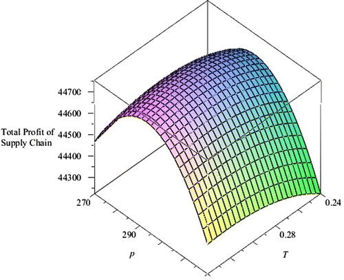
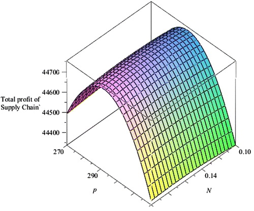
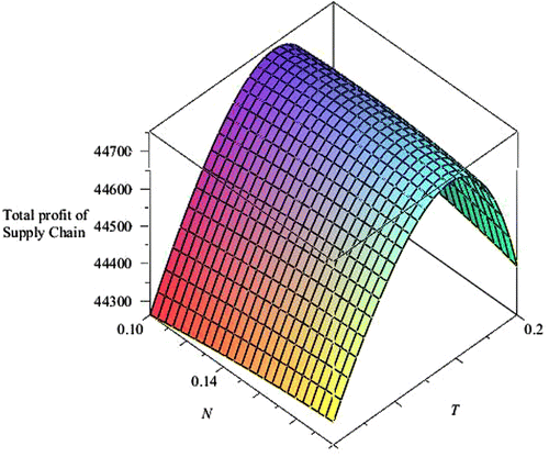
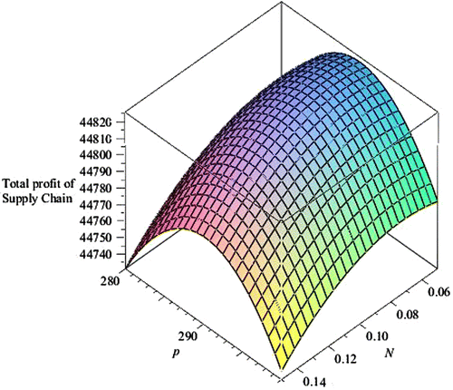
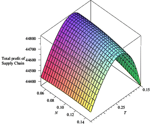
α = 300, β = 5, η = 0.5, δ = 0.40, τ = 0.75, λ = 0.03, θ = 0.15, A_r = 150, A_m = 300, h_r = 0.3, h_m = 0.5, C_r = 40, C_m = 10, p = 1000, I_e = 9%, I_b = 15%, I_lm = 18%, M = 0.3 in appropriate units. The maximum profit is π₁ = $44754.29 for cycle time T = 0.304 years by giving credit period N = 0.156 years to the customer at retail price p = $292.13 per unit. For obtained values:

$\left|\begin{array}{ccc}\frac{{\mathit{\partial }}^2{\mathit{\pi }}_1}{\mathit{\partial }{T}^2}& \frac{{\mathit{\partial }}^2{\mathit{\pi }}_1}{\mathit{\partial }T\mathit{\partial }p}& \frac{{\mathit{\partial }}^2{\mathit{\pi }}_1}{\mathit{\partial }T\mathit{\partial }N}\\ \frac{{\mathit{\partial }}^2{\mathit{\pi }}_1}{\mathit{\partial }T\mathit{\partial }p}& \frac{{\mathit{\partial }}^2{\mathit{\pi }}_1}{\mathit{\partial }{p}^2}& \frac{{\mathit{\partial }}^2{\mathit{\pi }}_1}{\mathit{\partial }p\mathit{\partial }N}\\ \frac{{\mathit{\partial }}^2{\mathit{\pi }}_1}{\mathit{\partial }T\mathit{\partial }N}& \frac{{\mathit{\partial }}^2{\mathit{\pi }}_1}{\mathit{\partial }p\mathit{\partial }N}& \frac{{\mathit{\partial }}^2{\mathit{\pi }}_1}{\mathit{\partial }{N}^2}\end{array}\right|=-6.623616594\times {10}^8<0$, 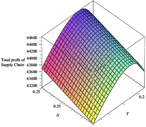suggesting the concavity of the profit. Figures 1^{Figure 2}–3 show concavity of the profit function with respect to two variables.

Figure 1. Concavity of total profit of the supply chain when N = 0.156 for N ≤ M ≤ T.

Figure 2. Concavity of total profit of the supply chain when T = 0.304 for N ≤ M ≤ T.

Figure 3. Concavity of total profit of the supply chain when p = 292.13 for N ≤ M ≤ T.

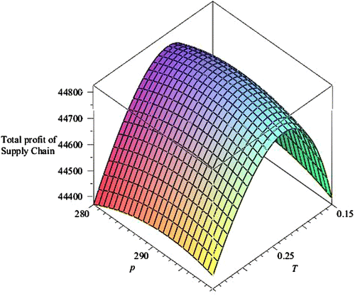
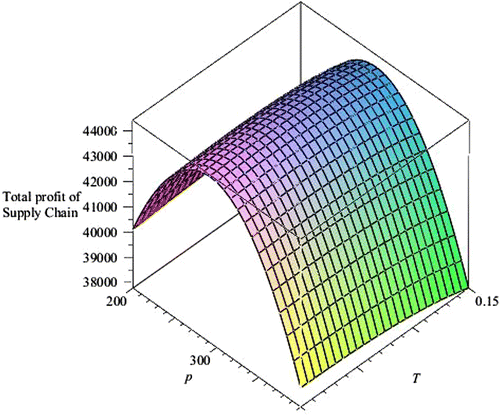
Example 2: Take β = 3 and other parametric values as given in Example 1. The scenario N ≤ T ≤ M gives maximum profit as π₂ = $44825.81 at N = 0.071, p = 290.05, T = 0.229. One can check the maximization of the profit for obtained values in a similar way as given in Example 1. Figures 4^{Figure 5}–6 show concavity of the profit function.

Figure 4. Concavity of total profit of the supply chain when N = 0.071 for N ≤ T ≤ M.

Figure 5. Concavity of total profit of the supply chain when N = 0.229 for N ≤ T ≤ M.

Figure 6. Concavity of total profit of the supply chain when p = 290.05 for N ≤ T ≤ M.

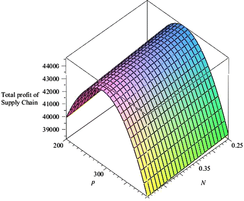
Example 3: Take β = 10 and M = 0.4 with other parametric values as given in Example 1 results profit to be π₃ = $44412.11 at N = 0.348, p = 293.66, T = 0.249 from the scenario T ≤ N ≤ M. One can check the maximization of the profit for obtained values in a similar way as given in Example 1. Figures 7^{Figure 8}–9 show concavity of the profit function.

Figure 7. Concavity of total profit of the supply chain when N = 0.348 for T ≤ N ≤ M.

Figure 8. Concavity of total profit of the supply chain when T = 0.249 for T ≤ N ≤ M.

Figure 9. Concavity of total profit of the supply chain when p = 293.66 for T ≤ N ≤ M.

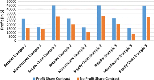
If the retailer does not offer credit period N to the customer, then the maximum profit is $43758.87 with selling price $247.83 and replenishment time 0.281 years using data as given in Example 1. The decrease in profit is due to decrease in demand. In Figure 10, we compare profit of the players and supply chain when sharing is considered and sharing is not considered.

Figure 10. Profit of the players in different scenario.

It is observed from Figure 10 that the retailer as an individual player has more profit as compared to manufacturer. This suggests that the retailer will like to be dominant player of the business transactions. To increase manufacturer profit, the strategy of profit sharing will be advantageous to both the players which results the better profit of the supply chain.

5. Sensitivity analysis

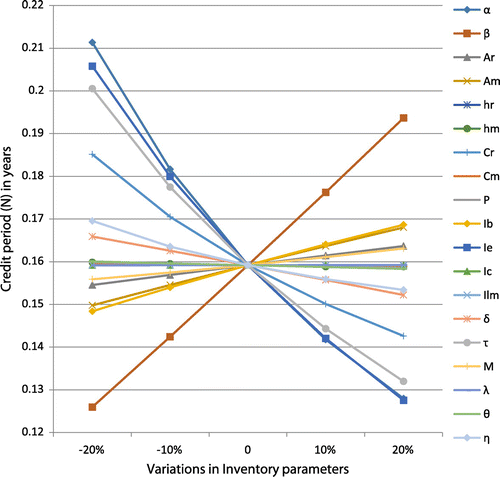
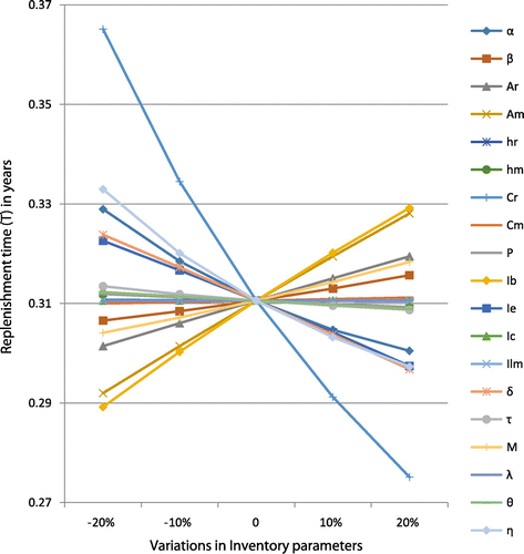
In this section, we consider the data given in Example 1. Varying one parameter at a time by −20%, −10%, + 10%, + 20%, we study its effects on optimal solutions and total profit of the supply chain. The changes in the trade credit, N offered by the retailer to the customer, retail price, p set by the retailer, cycle time, T and joint profit of the whole system are studied.

From Figure 11 it is observed that increase in scale demand decreases credit period offered to the customer by the retailer significantly. Similar observations are for profit sharing fraction, rate of interest earned, and price elasticity markup. It also suggests that the retailer’s purchase cost decreases the credit period. This supports that the customers will be attracted if they have to pay less as the purchase cost. The interest on the bank loan increases the credit period because this will facilitate the retailer to elongate the settlement of the payment.

Figure 11. Changes in credit period N with variations in inventory parameters.

Figure 12 depicts variations in the cycle time with respect to variations in inventory parameters. Increase in retailer’s purchase cost decreases cycle time significantly. The scale demand, price elasticity markup, profit sharing fraction, and interest earned reduces the cycle time of the supply chain. The bank interest and setup cost incurred by the manufacturer increases the cycle time. This suggests that both the players should have proper sharing information to stabilize the trade-off between retailer’s ordering quantity and manufacturer’s setup cost. The retailer should try to reduce the loan amount for settlement of the accounts against the purchases.

Figure 12. Changes in replenishment time with variations in inventory parameters.

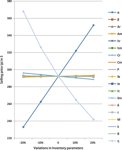
The selling price is positively sensitive to scale demand and negatively sensitive to price markup and retailer’s purchase cost as shown in Figure 13. Other inventory parameters have standard impact as discussed by cited articles in the references.

Figure 13. Changes in selling price with variations in inventory parameters.

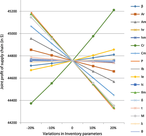
Figure 14 is about profit variations with respect to inventory parameters. The retailer’s purchase cost set by the manufacturer increases joint profit significantly. The credit period offered by the manufacturer to the retailer decreases the profit of the supply chain. The profit decreases with increase in the production rate. This suggests that the manufacturer and retailer should work on the production rate, credit period, and retailer’s purchase cost to increase the profit of the supply chain. This strategy will also control the setup cost of manufacturer. The retailer should put large order to save in ordering cost and as a result profit of the supply chain can be increased significantly. It is observed that increase in customer eligible for delay payments results decrease in the profit of the supply chain.

Figure 14. Changes in profit of supply chain with variations in inventory parameters.

6. Conclusions

This study deals with two-level trade credit financing for two players of the supply chain viz. manufacturer and the retailer. The market demand is dependent on retail price and credit period offered to the customer by the retailer. The study considers sharing of profit between the players during the credit period. The units in inventory system are subject to deterioration at a constant rate. Numerically, it is observed that a two-level trade credit strategy with profit sharing contract increases profit of both the players and also that of the supply chain. The proposed model can be extended to incorporate preservation technology investment to control the deterioration of items in the inventory system. The problem can be studied for stochastic demand which will explore real market practices.

Acknowledgments

Author likes to thank anonymous reviewers’ suggestions for improvement of the readability of the manuscript. The department is under the scheme of DST-FIST.

Additional information

Funding

Funding. The author received no direct funding for this research.

Notes on contributors

Nita H. Shah

Nita H. Shah is a professor in the Department of Mathematics, Gujarat University, Ahmadabad, India. She holds a PhD in Inventory Control Management, Operations Research. Currently, she is engaged in research in inventory control and management, supply chain management, forecasting and information technology and information systems, neural networks, and sensors and image processing. She has more than 275 papers published in international and national journals. She is author of four books. She is serving as a member of the editorial board of Investigation Operational, Journal of Social Science and Management, International Journal of Industrial Engineering and Computations and Mathematics Today.

References

- Abad, P. L., & Jaggi, C. K. (2003). A joint approach for setting unit price and the length of the credit period for a seller when end demand is price sensitive. International Journal of Production Economics, 83, 115–122.10.1016/S0925-5273(02)00142-1
- Chang, C. T., Teng, J. T., & Goyal, S. K. (2008). Inventory lot-size models under trade credits: A review. Asia-Pacific Journal of Operational Research, 25, 89–112.10.1142/S0217595908001651
- Chen, H., Chen, Y. H., Chiu, C. H., Choi, T. M., & Sethi, S. (2010). Coordination mechanism for the supply chain with leadtime consideration and price-dependent demand. European Journal of Operational Research, 203, 70–80.10.1016/j.ejor.2009.07.002
- Chen, L. H., & Kang, F. S. (2007). Integrated vendor–buyer cooperative inventory models with variant permissible delay in payments. European Journal of Operational Research, 183, 658–673.10.1016/j.ejor.2006.10.035
- Chen, L. H., & Kang, F. S. (2010a). Integrated inventory models considering the two-level trade credit policy and a price-negotiation scheme. European Journal of Operational Research, 205, 47–58.10.1016/j.ejor.2009.11.028
- Chen, L. H., & Kang, F. S. (2010b). Coordination between vendor and buyer considering trade credit and items of imperfect quality. International Journal of Production Economics, 123, 52–61.10.1016/j.ijpe.2009.06.043
- Chen, S. C., Teng, J. T., & Skouri, K. (2014). Economic production quantity models for deteriorating items with up-stream full trade credit and down-stream partial trade credit. International Journal of Production Economics, 155, 302–309.10.1016/j.ijpe.2013.07.024
- Chiu, C. H., Choi, T. M., & Li, D. (2009). Price wall or war: The pricing strategies for retailers. IEEE Transactions on Systems, Man, and Cybernetics, Part A—Systems and Humans, 39, 331–343.10.1109/TSMCA.2008.2010753
- Chiu, C. H., Choi, T. M., & Tang, C. S. (2011). Price, rebate, and returns supply contracts for coordinating supply chains with price-dependent demands. Production and Operations Management, 20, 81–91.10.1111/poms.2010.20.issue-1
- Chung, K. J., & Cárdenas-Barrón, L. E. (2013). The simplified solution procedure for deteriorating items under stock-dependent demand and two-level trade credit in the supply chain management. Applied Mathematical Modelling, 37, 4653–4660.10.1016/j.apm.2012.10.018
- Chung, K. J., Cárdenas-Barrón, L. E., & Ting, P. S. (2014). An inventory model with non-instantaneous receipt and exponentially deteriorating items for an integrated three layer supply chain system under two levels of trade credit. International Journal of Production Economics, 155, 310–317.10.1016/j.ijpe.2013.12.033
- Feng, X., Moon, I., & Ryu, K. (2014). Revenue-sharing contracts in an N-stage supply chain with reliability considerations. International Journal of Production Economics, 147, 20–29.10.1016/j.ijpe.2013.01.002
- Giri, B. C., & Maiti, T. (2013). Supply chain model with price- and trade credit sensitive demand under two-level permissible delay in payments. International Journal of Systems Science, 44, 937–948.10.1080/00207721.2011.649367
- Goyal, S. K. (1985). Economic order quantity under conditions of permissible delay in payments. Journal of the Operational Research Society, 36, 335–338.10.1057/jors.1985.56
- He, Y., & Huang, H. (2013). Two-level credit financing for noninstantaneous deterioration items in a supply chain with downstream credit-linked demand. Discrete Dynamics in Nature and Society, 917958, 22. doi:10.1155/2013/917958
- Ho, C. H., Ouyang, L. Y., & Su, C. H. (2008). Optimal pricing, shipment and payment policy for an integrated supplier–buyer inventory model with two-part trade credit. European Journal of Operational Research, 187, 496–510.10.1016/j.ejor.2007.04.015
- Huang, Y. F. (2003). Optimal retailer’s ordering policies in the EOQ model under trade credit financing. Journal of the Operational Research Society, 54, 1011–1015.10.1057/palgrave.jors.2601588
- Huang, Y. F. (2006). An inventory model under two levels of trade credit and limited storage space derived without derivatives. Applied Mathematical Modelling, 30, 418–436.10.1016/j.apm.2005.05.009
- Huang, Y. F. (2007). Optimal retailer’s replenishment decisions in the EPQ model under two levels of trade credit policy. European Journal of Operational Research, 176, 1577–1591.10.1016/j.ejor.2005.10.035
- Huang, Y. F. (2008). An EOQ model under retailer partial trade credit policy in supply chain. International Journal of Production Economics, 112, 655–664.10.1016/j.ijpe.2007.05.014
- Huang, C. K., Tsai, D. M., Wu, J. C., & Chung, K. J. (2010). An integrated vendor–buyer inventory model with order-processing cost reduction and permissible delay in payments. European Journal of Operational Research, 202, 473–478.10.1016/j.ejor.2009.05.035
- Jaber, M. Y., & Osman, I. H. (2006). Coordinating a two level supply chain with delay in payments and profit sharing. Computers & Industrial Engineering, 50, 385–400.
- Jaggi, C. K., Goyal, S. K., & Goel, S. K. (2008). Retailer’s optimal replenishment decisions with credit-linked demand under permissible delay in payments. European Journal of Operational Research, 190, 130–135.10.1016/j.ejor.2007.05.042
- Jiang, W., Ouyang, L. Y., Cárdenas-Barrón, L. E., & Goyal, S. K. (2014). Optimal credit period and lot size for deteriorating items with expiration dates under two-level trade credit financing. European Journal of Operational Research, 237, 898–908.
- Jiang, W., Skouri, K., Teng, J. T., & Ouyang, L. Y. (2014). A note on “optimal replenishment policies for non-instantaneous deteriorating items with price and stock sensitive demand under permissible delay in payment”. International Journal of Production Economics, 155, 324–329.
- Kim, J., Hong, Y., & Kim, T. (2011). Pricing and ordering policies for price-dependent demand in a supply chain of a single retailer and a single manufacturer. International Journal of Systems Science, 42, 81–89.10.1080/00207720903470122
- Liao, J. J. (2008). An EOQ model with noninstantaneous receipt and exponentially deteriorating items under two-level trade credit. International Journal of Production Economics, 113, 852–861.10.1016/j.ijpe.2007.09.006
- Ouyang, L. Y., Ho, C. H., & Su, C. H. (2008). Optimal strategy for an integrated system with variable production rate when the freight rate and trade credit are both linked to the order quantity. International Journal of Production Economics, 115, 151–162.10.1016/j.ijpe.2008.04.012
- Sarmah, S. P., Acharya, D., & Goyal, S. K. (2007). Coordination and profit sharing between a manufacturer and a buyer with target profit under credit option. European Journal of Operational Research, 182, 1469–1478.10.1016/j.ejor.2006.09.047
- Shah, N. H., Shukla, K. T., & Shah, B. J. (2009). Deteriorating inventory model for two-level credit linked demand under permissible delay in payment. Australian Society of Operational Research Bulletin, 28, 27–36.
- Shah, N. H., Soni, H., & Jaggi, C. K. (2010). Inventory models and trade credit: Review. Control & Cybernetics, 39, 867–884.
- Sheen, G. J., & Tsao, Y. C. (2007). Channel coordination, trade credit and quantity discounts for freight cost. Transportation Research Part E: Logistics and Transportation Review, 43, 112–128.10.1016/j.tre.2005.08.001
- Teng, J. T., Chang, C. T., & Chem, M. S. (2012). Vendor–buyer inventory models with trade credit financing under both non-cooperative and integrated environments. International Journal of Systems Science, 43, 2050–2061. doi:10.1080/00207721.2011.564322
- Teng, J. T., Chang, C. T., Chern, M. S., & Chan, Y. L. (2007). Retailer’s optimal ordering policies with trade credit financing. International Journal of Systems Science, 38, 269–278.10.1080/00207720601158060
- Teng, J. T., & Goyal, S. K. (2007). Optimal ordering policies for a retailer in a supply chain with up-stream and down-stream trade credits. Journal of the Operational Research Society, 58, 1252–1255.10.1057/palgrave.jors.2602404
- Yen, G. F., Chung, K. J., & Chen, T. C. (2012). The optimal retailer’s ordering policies with trade credit financing and limited storage capacity in the supply chain system. International Journal of Systems Science, 43, 2144–2159. doi:10.1080/00207721.2011.565133