Calibration of safety performance function for crashes on inter-city four lane highways in India

Abstract

There is a significant need to improve the highway safety during roadway planning, design and operations in developing countries like India. To receive appropriate consideration, safety needs to be dealt objectively within the transportation planning and highway design processes. Lack of available tools is a deterrent to quantify safety of a transportation facility during the planning or highway design process. The objective of this paper is to develop safety performance functions considering various elements involved in the planning, design and operation of a section on four-lane National Highway (NH)-58 located in the state of Uttarakhand, India. The mixed traffic on Indian multilane highways comes with a lot of variability within, ranging from different vehicle types to different driver characteristics. This could result in variability in the effect of explanatory variables on crashes across locations. Hence, explanatory variables for highway segment safety analysis considered were geometric characteristics like curvature change rate, slope change rate, transverse slope and traffic characteristics in the form of average daily traffic, light vehicle traffic, light commercial vehicle traffic, heavy vehicle traffic, two-wheelers, non-motorised traffic volume and operating speed were analysed against dependent variable as crash count per 200 m per year. Safety performance functions involving the explanatory variables are calibrated to predict crash frequency using Poisson Weibull technique and crash types are predicted using ordered logit model. Model results suggest that increase in traffic volume leads to higher probability of crash risk and traffic safety is significantly distorted by higher curvature change rate values.

Keywords:

• crash frequency
• crash type
• Poisson Weibull
• Bayesian inference
• ordered logit model

Public Interest Statement

In this study, we develop safety performance functions considering various elements involved in the planning, design and operation of four-lane national highways in India. Explanatory variables for highway segment safety analysis considered were geometric characteristics and traffic characteristics analysed against dependent variable as crash count and collision type. Safety performance functions involving the explanatory variables are calibrated to predict crash frequency using Poisson Weibull technique and crash types are predicted using ordered logit model. Model results suggest that increase in traffic volume leads to higher probability of crash risk and traffic safety is significantly distorted by higher curvature change rate values.

1. Introduction

Over the years due to growth in Indian economy, there has been an unprecedented increase in road transportation and vehicular traffic load on the existing highway network in India, which has led to unsafe conditions on our highways. Casualties due to crashes on these roads are increasing year after year. The road safety is further deteriorated by poor maintenance of vehicle, bad driving practice, lack of enforcement, casual attitude of road users and least concern towards the basic road safety measures by road maintaining agencies.

At present in India, more than 486,476 crashes occur annually. About 137,572 people lose their lives in such crashes. Additionally, nearly 494,893 people get injured in road crashes that lead to lifelong misery for the victims and family (Road Accidents in India, 2014). Road Safety Study can ensure that various safety deficiencies in road are reviewed so that these can be taken care at appropriate stage of road design or operation and maintenance of road in a cost-effective way. In recent years, significant effort and investment have been made to enhance highway safety. In the backdrop of resource constraints, the allocation of resources for safety improvement projects must yield maximum possible return on investment. Identifying highway locations that have the potential for crash reduction with the implementation of effective safety counter measures is therefore an important step in achieving the maximum return on safety investment.

Considerable amount of research has been done in recent years for developed countries to establish relationships between crashes and various traffic flow characteristics, geometric characteristics at highway segments and intersections. Understanding of crash-contributing factors on highway system using recent scientific approaches is yet to take off in developing countries.

Miaou and Lum (1993) investigated statistical of four regression models—two conventional linear regression models and two Poisson regression models considering highway geometric design parameters. Study revealed that Poisson regression models overestimate or underestimate the crash frequency. Miaou (1994) evaluated the performance of Poisson, zero-inflated Poisson and negative binomial regression models through maximum likelihood method to predict truck crashes in relation with road geometric parameters. Hauer (1997) describes various conventional approaches for statistical analysis of road safety engineering. Empirical Bayes (EB) approach to the analysis of road accident data is explained extensively. EB approach was adopted to eliminate the bias in estimated accident rates that arise from selection criteria. Persaud, Lord, and Palmisano (2002) studied the transferability of safety performance functions or crash prediction models to other jurisdictions. Study suggested that a single calibration factor is inappropriate and that a disaggregation by traffic volume is preferred.

Miaou and Lord (2003) analysed traffic crashes with respect to traffic flows at intersections. They challenged the assumption of fixed dispersion parameter and worked with various dispersion parameter relationships and functional forms. This study also indicated the advantages of full Bayes versus EB method. Mitra and Washington (2007) developed eight different models with explanatory factors as traffic flow and geometric factors to estimate crashes. Study suggested that model specification may be improved by testing extra variation functions for significance.

Geedipally and Lord (2008) evaluated the safety performance functions using a varying dispersion parameter which precisely estimated crashes with smaller confidence intervals. Geedipally and Lord (2010) investigated crashes as per single- and multi-vehicle crashes separately versus modelling total crash frequency. Cheng, Geedipally, and Lord (2013) evaluated the application of Poisson Weibull (PW) and Poisson Gamma (PG) models and results revealed both the techniques are competitive.

Numerous studies have been performed by many researchers on road safety analysis in India. Landge (2006) reviewed different modelling approaches adopted worldwide. Dinu and Veeraragavan (2011) implemented random parameters count model. The results suggested that the model coefficients for traffic volume, proportion of cars, motorised two-wheelers (TW) and trucks in traffic, and driveway density and horizontal and vertical curvatures are randomly distributed across the locations. Krishnan, Anjana, and Anjaneyulu (2013) applied hierarchical modelling approach to estimate crash frequency and severity of single and dual carriageway roads. Research review illustrated that the safety performance of non-urban four-lane highways was seldom investigated on Indian highways. The review indicated that there is a need to develop models for estimating the safety performance of non-urban highways using recent statistical techniques adopted in developed countries.

The study aims to (1) identify the crash contributing factors and (2) to develop safety performance functions using Bayesian inference to predict crash frequency and different crash types on a section of divided four-lane National Highway-58 in India.

2. Study approach

Real-world crash data that are properly defined can identify the key contributing factors to traffic crashes in terms of crash frequency (number of crashes per segment), crash type (direct impact collision, rear-end collision, sideswipe collision, rollover collision and skid-related collisions) and crash severity (fatal, incapacitating, non-incapacitating, animal-related crashes and property damage only). Hence, for scientific research on crashes, one first needs to have a reliable crash database. In India, there is no organised crash database maintained for in-depth research on crashes. The absence of such nationwide systematic data, seriously impede the scientific research and analysis of road crashes in India. To address this issue and to identify the root cause of crashes in India, it is necessary to fully understand the traffic and crash affecting parameters. Hence, in this study, an attempt is made to create the crash database for scientific research on crashes on four-lane divided national highway.

2.1. Study area description

The National Highway-58 connects Indian capital New Delhi to Mana, near China border in Uttrakhand state. It serves as a lifeline to the hilly part of the state. The road is strategically important being the shortest route from Delhi to international China border. The highway has length of 536 km of which 230-km length in plain and rest in the hilly terrain. The highway connects important religious destinations which attract tourists from all over the country and world throughout the year. The highway has two-lane and four-lane stretches. Traffic on the highway is mixed in nature and comprises heavy and light vehicles. Most of the highway study segment falls in rural areas (approximately 85%).

2.2. Site selection

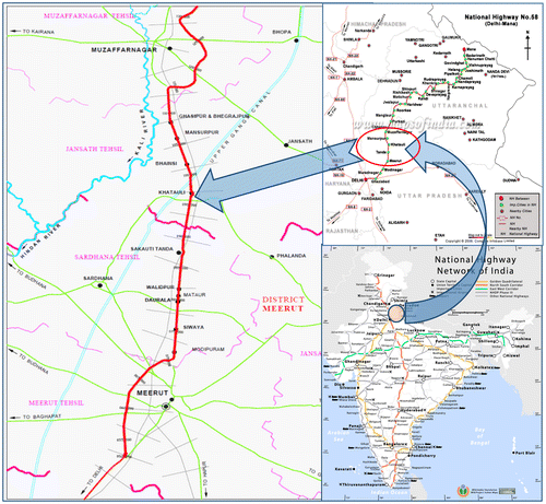
This national highway is maintained and operated by National Highway Authority of India (NHAI) and concessionaire Western Uttar Pradesh Toll Ltd (WUPTL). The study has been done for four-lane road between km 52.00 and 130.00 to identify all safety deficiencies responsible for road crashes. Route map of study section of National Highway-58 is shown in Figure 1.

Figure 1. Study area route map of National Highway-58.

2.3. Details of road geometrics

Figure 2 shows typical cross-section of the candidate stretch under analysis. Table 1 shows the road infrastructure details for the study area. As per Indian Roads Congress (2000), the ruling design speed for National Highway-58 in plain terrain is 100 kmph.

Figure 2. Typical cross-section for four-lane National Highway-58.

Note: All dimensions in millimeter.

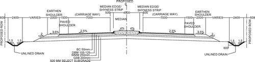
Table 1. Road infrastructures details

Highway features	Description/Quantity
Grade separated junctions	07 numbers
At-grade junctions	08 numbers
Major bridges	02 numbers
R O B	02 numbers at km 87.583 and 114.289
Underpasses	05 numbers at km 78.815, 87.400, 102.896, 118.550 and 122.175
Culverts	186 numbers
Truck lay byes	02 numbers
Bus lay bays	07 numbers
Toll plaza	1 number at km 75.990

2.4. Crash database description

From past studies, it is evident that any crash is a resultant of deficiency in any one of these factors, highway design, driver behaviour and vehicle defect. Hence, there are number of associated parameters for each of these aforementioned three factors leading to the occurrence of crashes and it is practically a challenging job to collect all these parameters. By considering the parameters applied in past crash prediction models and practical availability of data, data were collected for estimating the crash prediction models. Crash records for three years from May 2011 to April 2014 were collected from various police stations along the study section and WUPTL. Highway as-built drawings revealing the plan and profile of the study stretch and average daily traffic (ADT) for the study period was obtained from NHAI.

Classified traffic volume count survey was carried out manually at km 89.00 (near Dadri village) on NH-58 for 24 h on 6 June 2013. Later video graphic traffic volume count for morning and evening peak two hours was conducted at 15 major intersections. Assumption was made that there are no entry and exit of major traffic in between these intersections. Different traffic volumes like major highway traffic, minor road traffic, major road crossing traffic, merging and diverging traffic details were retrieved at each intersection from these video data using a C program.

2.5. Crash pattern and candidate segment

Total crash count (CC) per kilometre for the study period under consideration is as shown in Figure 3. Crash severity (for both intersection and segment crashes) and collision type (for segment crashes) statistics for the analysis period are revealed in Tables 2 and 3, respectively. From this, we can visualise that there are more than 20 crashes per kilometre throughout the analysis period along the study stretch. Safety performance functions were developed for crashes occurring on the highway segments only. Crashes occurring within a circle of 76 m (250 feet) were considered as intersection crash (Lord et al., 2008) and were excluded from the analysis data. Hence, there were 60 major segments (both directional) which were further divided into 200-m stretches. A minimum segment length of 0.1 mile (≈161 m) (American Association of State Highway and Transportation Officials, 2010; Miaou, 1994) was considered to avoid low-exposure criteria and large statistical uncertainty of CC per short segment. Segments shorter than 162 m were combined with the neighbouring segments with comparably similar geometrical characteristics.

Figure 3. Total CC per kilometre along the study stretch.

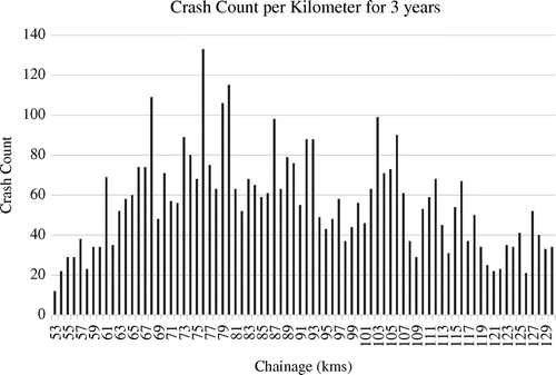
Table 2. Crash severity statistics for the study stretch

Time period	Fatal	Incapacitating injury	Non-incapacitating injury	Property damage	Animals killed	Total crashes
2011	66	237	293	365	378	1,339
2012	92	185	423	498	334	1,532
2013	81	198	361	451	399	1,490
Grand total	239	620	1,077	1,314	1,111	4,361
Share (%)	5.48	14.22	24.70	30.13	25.48	100

Table 3. Collision-type statistics of segment crashes along the study stretch

Time period	Direct impact collision (DI)	Rear end collision (REC)	Sideswipe collision (SSC)	Rollover collision (ROC)	Skidding collision (SKC)	Total segment crashes
2011	452	435	163	72	102	1,224
2012	460	478	157	80	202	1,377
2013	449	470	258	43	213	1,433
Grand total	1,361	1,383	578	195	517	4,034
Share (%)	31.21	31.71	13.25	4.47	11.86	100

2.6. Influencing variables

CC per 200 m per year was taken as dependent variable in the crash prediction models. The safety parameters included in study were geometric characteristics like curvature change rate (CCR), slope change rate (SCR), transverse slope (TS) and traffic characteristics as ADT, traffic composition-like car (CAR) [composing cars, three- and four-wheeler autos], SUV, minibus, bus, light commercial vehicles (MTRUCK), heavy traffic volume (HTV) [two-axle trucks, multi-axle trucks, tractor-trailers], two-wheelers (TW) and non-motorised traffic volume (NMTV) [cycles, cycle rickshaws, animal-driven carts] and operating speed, V₈₅ (American Association of State Highway and Transportation Officials, 2004; Jacob & Anjaneyulu, 2013) of vehicles in the traffic stream. For convenient calculations, natural log of traffic volume, speed, segment length and composition of vehicles was included in the models.

Curvature treated as CCR (Lamm, Wolhuter, Beck, & Rusher, 2001) of the segment, calculated as follows:(1) $$\text{CCR}[\text{gon}/\text{m}]=\frac{{\sum }_i\left|{\mathit{\gamma }}_i\right|}{L}$$(1)

where γ_i is the deflection angle for a contiguous element (curve or tangent) i within a section of length L.

Tables 4 and 5 give the statistical summary of the variables selected to build the safety performance functions for crash frequency and crash-type prediction, respectively. The results in Table 4 revealed that for any subset of the independent variables, the CC exhibits overdispersion.

Table 4. Statistical summaries of NH-58 crash data used in crash prediction models

Variable	Mean	Std. Dev.	Minimum	Maximum	Total
Total crashes	1.922	2.069	0	18	4,037
Segment length (m)	204.761	23.754	162	350	143,333
CCR (gon/m)	0.024	0.038	0	0.318	–
TS (%/m)	−2.048	2.353	−7	7	–
SCR (gon/m)	0.016	0.210	−1.589	1.543	–
Speed (kmph)	85.182	5.207	75.9	95	–
MO (no./segment)	0.087	0.282	0	1	61
ADT (veh/day)	23,027.662	6,006.542	13,563	40,936	–
CAR (veh/day)	10,276.515	2,935.922	5,056	19,264	–
SUV (veh/day)	3,063.441	921.151	1,409	6,838	–
MBUS (veh/day)	240.584	111.594	69	569	–
MTRUCK (veh/day)	6,034.901	2,241.029	2,664	12,208	–
BUS (veh/day)	730.959	287.526	357	1,793	–
HTV (veh/day)	1,538.635	1,106.875	693	6,693	–
TW (veh/day)	534.711	169.224	231	1,146	–
NMTV (veh/day)	608.405	357.652	35	1,523	–

Notes: Total Crashes (CC), Segment Length (Offset, meters), Curvature Change Rate (CCR), Slope Change Rate (SCR), Transverse Slope (TS), Operating Speed of Traffic (Speed), Median opening (MO), Average Daily Traffic (ADT), Cars (CAR), Sport Utility Vehicles (SUV), Minibuses (MBUS), Minitrucks (MTRUCK), Buses (BUS), Heavy Traffic Volume (HTV), Two-Wheelers (TW) and Non-motorised Traffic Volume (NMTV).

Table 5. Statistical summaries of NH-58 crash data used in crash severity model

Variable	Mean	Std. Dev.	Minimum	Maximum	Total
Direct impact collision (Code: 1)	–	–	–	–	1,361
Rear end collision (Code: 2)	–	–	–	–	1,383
Sideswipe collision (Code: 3)	–	–	–	–	5,78
Rollover collision (Code: 4)	–	–	–	–	5,17
Skidding collision (Code: 5)	–	–	–	–	195
Crash type levels	2.207	1.177	1	5	8,904
Segment length (m)	210.9	34.18495	162	350	850,621
CCR (gon/m)	0.02442	0.036	0	0.318	–
SCR (gon/m)	0.0154	0.215	−1.589	1.543	–
TS (%/m)	−2.14	2.232	−7	7	–
Speed (kmph)	84.55	5.289	75.9	95	–
MO (no./segment)	0.1326	0.339	0	1	535
ADT (veh/day)	23,383	6,158.987	13,563	40,936	–
CAR (veh/day)	10,346	3,055.177	5,057	19,263	–
SUV (veh/day)	3,089	870.2998	1,409	6,836	–
MBUS (veh/day)	233.39	101.3184	68	568.29	–
MTRUCK (veh/day)	542.2	176.0962	230.9	1,145.1	–
BUS (veh/day)	745.7	260.21	356.0	1,792	–
HTV (veh/day)	1,443.5	985.5002	693.5	6,694	–
TW (veh/day)	6,329	2,212.998	2,664	12,209	–
NMTV (veh/day)	654.41	374.6066	35	1,523	–
Day (Type coded 1–7)	3.994	2.03946	1	7	–
Time (Coded 1–24)	12.46	6.517811	1	24	–
AHT (°C)	32.13	5.937391	21.00	41.00	–
ALT (°C)	18.5	7.45330	7.0	28.0	–
PRCPTN (mm)	2.204	8.512072	0.00	123.00	–

Notes: Segment Length (Offset, meters), Curvature Change Rate (CCR), Slope Change Rate (SCR), Transverse Slope (TS), Operating Speed of Traffic (Speed), Median opening (MO), Average Daily Traffic (ADT), Cars (CAR), Sport Utility Vehicles (SUV), Minibuses (MBUS), Minitrucks (MTRUCK), Buses (BUS), Heavy Traffic Volume (HTV), Two-Wheelers (TW) and Non-motorised Traffic Volume (NMTV), Day-type (Day), Daily average high temperature (AHT), Daily average low temperature (ALT) and Precipitation (PRCPTN).

2.7. Model formulation and analysis

Two model forms were considered for analysis as per ease of access to required data, as in most of the situation in India, it is a challenging job to collect crash records, geometric design parameters and other variables for crash analysis.

The following generalized linear model functional form has been used in all Bayesian analyses:

Model A:(2) $${\mathit{\mu }}_{ij}=\text{exp}(\text{Alpha}+B[2]{\text{ADT}}_{ij}+{\text{Offset}}_i)$$(2)

Model B:(3) $${\mathit{\mu }}_{ij}=\text{exp}(\text{Alpha}+B\left[2\right]CC{R}_i+B\left[3\right]SC{R}_i+B\left[4\right]T{S}_i+B\left[5\right]Spee{d}_i+B\left[6\right]M{O}_i+B[7]{\text{CAR}}_{ij}+B[8]{\text{SUV}}_{ij}+B[9]{\text{MBUS}}_{ij}+B[10]{\text{MTRUCK}}_{ij}+B[11]{\text{BUS}}_{ij}+B[12]{\text{HTV}}_{ij}+B[13]{\text{TW}}_{ij}+B[14]{\text{NMTV}}_{ij}+{\text{Offset}}_i)$$(3)

3. Modelling methodology applied

3.1. Poisson–Weibull (PW) model

As the name suggests, PW distribution is a mixture of Poisson and Weibull distribution. PW model is similar to most Poisson-based distributions (e.g. Poisson-gamma and Poisson-lognormal), it is also designed to accommodate the overdispersion. Interested readers are referred to Cheng et al. (2013) for further detailed information. The number of crashes “Y_it” for a particular ith site and time period t when conditional on its mean μ_it is Poisson distributed and independent over all sites and time periods.(4) $$Y_{it}|{\mathit{\mu }}_{it}\sim \text{Poisson}({\mathit{\mu }}_{it})\text{where},i=1,2,\dots ,I\text{and}t=1,2,\dots T$$(4)

The mean of the Poisson is structured as:(5) $${\mathit{\mu }}_{it}=\widehat{{\mathit{\mu }}_{it}}{\mathit{\epsilon }}_{it}=f\left(X;\mathit{\beta }\right)·{\mathit{\epsilon }}_{it}$$(5) (6) $$\widehat{{\mathit{\mu }}_{it}}=f\left(X;\mathit{\beta }\right)=exp\left({\mathit{\beta }}_0+\sum _{j=1}^q{\mathit{\beta }}_j{X}_{jt}\right)\text{where},j=1,2,3\dots q\text{and}t=1,2,3$$(6) (7) $${\mathit{\epsilon }}_{it}\sim \text{Weibull}(v,\mathit{\lambda })$$(7)

where f (·) is a function of the covariates (X); β is a vector of unknown regression coefficients; and ε_it is the model error independent of all the covariates.

In PW model, it is assumed that ε_it is independent and Weibull distributed. The Weibull probability density function (p.d.f) is given as follows:(8) $$f(x)=\frac{v}{\mathit{\lambda }}{\left(\frac{x}{\mathit{\lambda }}\right)}^{v-1}exp\left[-{\left(\frac{x}{\mathit{\lambda }}\right)}^v\right];x>0,v>0,\mathit{\lambda }>0$$(8)

where λ and v are scale and shape parameters, respectively. The p.d.f. of the Weibull distribution can fit to various shapes similar to that of the gamma, gamma-like, exponential or approximate normal distributions depending on the v values. This characteristic of PW model provides a lot of flexibility to fit different kinds of data.

The mean and variance of the Weibull distribution are:(9) $$E(\mathit{\epsilon })=\mathit{\lambda }\left(1+\frac{1}{v}\right)$$(9) (10) $$\text{Var}(\mathit{\epsilon })={\mathit{\lambda }}^2\mathrm{\Gamma }\left(1+\frac{2}{v}\right)-{\left[\mathit{\lambda }\mathrm{\Gamma }\left(1+\frac{1}{v}\right)\right]}^2$$(10)

The PW distribution is defined as the mixture of Poisson and Weibull distributions such that(11) $$P\left(Y=y;\mathit{\mu },\mathit{\lambda },v\right)=\int \text{Poisson}(y;\widehat{\mathit{\mu }}\mathit{\epsilon })\text{Weibull}(\mathit{\epsilon };\mathit{\lambda },v)d\mathit{\epsilon }$$(11)

The mean or expected value of the PW distribution is given as:(12) $$E\left(Y\right)=\widehat{\mathit{\mu }}E\left(\mathit{\epsilon }\right)=\widehat{\mathit{\mu }}\times \left[\mathit{\lambda }\mathrm{\Gamma }\left(1+\frac{1}{v}\right)\right]$$(12)

and the variance is given by:(13) $$\text{Var}\left(Y\right)=\widehat{\mathit{\mu }}\times \left[\mathit{\lambda }\mathrm{\Gamma }\left(1+\frac{1}{v}\right)\right]+{\widehat{\mathit{\mu }}}^2\times {\mathit{\lambda }}^2\mathrm{\Gamma }\left(1+\frac{2}{v}\right)-{\widehat{\mathit{\mu }}}^2\times {\left[\mathit{\lambda }\mathrm{\Gamma }\left(1+\frac{1}{v}\right)\right]}^2$$(13)

3.2. Bayesian-ordered logit model

The ordered logit model is commonly implemented to analyse ordered categorical data (Greene, 2007; Xie, Zhang, & Liang, 2009; Ye & Lord, 2014). The ordered logit model uses a latent variable y*, as shown below to determine the different crash-type outcomes.(14) $$y_i^{*}=\mathit{\beta }{X}_i+{\mathit{\epsilon }}_i$$(14)

where X is a vector of independent variables for individual crashes; β is a vector of the unknown coefficients for these variables; and ε is a random error term assumed to follow standard normal distribution across observations.

Using Equation 10, the value of the crash-type variable y_i is estimated by:(15) $$y_i=\left\{\begin{array}{ccc}1,\hfill & \text{if}& y_i^{*}\le {\mathit{\gamma }}_1\\ k,\hfill & \text{if}& {\mathit{\gamma }}_{k-1}<y_i^{*}\le {\mathit{\gamma }}_k\\ C,\hfill & \text{if}& {\mathit{\gamma }}_{C-1}<y_i^{*}\end{array}\right.$$(15)

where $\mathit{\gamma }=\{{\mathit{\gamma }}_1,\dots ,{\mathit{\gamma }}_k,\dots {\mathit{\gamma }}_{C-1}\}$ are the threshold values for all crash severity levels coded as integers in order; k = 1, … , C (C = 5 in the paper), the five crash types under consideration are: 1 = direct impact collision (DI), 2 = rear-end collision (REC), 3 = sideswipe collision (SSC), 4 = rollover collision (ROC) and 5 = skidding collision (SKC); C is the highest ordered crash-type level.

Given the value of X_i, the probability of a crash category for an individual ith crash belonging to each category is(16) $$\left.\begin{array}{c}P(y_i=1)=\frac{exp(\mathit{\beta }{X}_i-{\mathit{\gamma }}_1)}{1+\left[exp(\mathit{\beta }{X}_i-{\mathit{\gamma }}_1)\right]}\hfill \\ P(y_i=k)=\frac{exp(\mathit{\beta }{X}_i-{\mathit{\gamma }}_{k-1})}{1+\left[exp(\mathit{\beta }{X}_i-{\mathit{\gamma }}_{k-1})\right]}-\frac{exp(\mathit{\beta }{X}_i-{\mathit{\gamma }}_k)}{1+\left[exp(\mathit{\beta }{X}_i-{\mathit{\gamma }}_k)\right]}\hfill \\ P(y_i=C)=1-\frac{exp(\mathit{\beta }{X}_i-{\mathit{\gamma }}_{C-1})}{1+\left[exp(\mathit{\beta }{X}_i-{\mathit{\gamma }}_{C-1})\right]}\hfill \end{array}\right\}$$(16)

3.3. Goodness-of-fit statistics

There are many measures that can be used for estimating how well the model fits the data. There are statistics for indicating the likelihood level of a model, that is, how well the model maximises the likelihood function. Among these statistics are:

3.3.1. Pearson chi-square

Another useful likelihood statistic is the Pearson chi-square and is defined as:(17) $$\text{Pearson}\text{-}{\mathit{\chi }}^2=\sum _{i=1}^N\frac{{(y_i-{\widehat{\mathit{\mu }}}_i)}^2}{\text{Var}(y_i)}$$(17)

3.3.2. Deviance information criterion

The deviance information criterion (DIC) (Congdon, 2006) calculation in WinBUGS was used as the measure for comparing the different Bayesian hierarchical models; DIC assigns a penalty for the complexity of the model.

The DIC for the jth model is given by:(18) $${\text{DIC}}_j=D({\overline{\mathit{\theta }}}_j)+2p{D}_j=\overline{D}+p{D}_j$$(18)

where $D({\overline{\mathit{\theta }}}_j)$ is the deviance $D({\overline{\mathit{\theta }}}_j|y)$ at the posterior mean ${\overline{\mathit{\theta }}}_j$ of the parameters for model j, called Dhat in WinBUGS, $\overline{D}$ is the expected deviance $\overline{D}=E(D|y,\mathit{\theta })$, given by the mean $\overline{D}$ of the sampled deviances D^(t) from Markov Chain Monte Carlo (MCMC) simulations, also called Dbar in WinBUGS, and pD_j is the effective number of parameters in the model, computed as the difference between ${\overline{D}}_j$ and $D({\overline{\mathit{\theta }}}_j)$, that is, $p{D}_j={\overline{D}}_j-D({\overline{\mathit{\theta }}}_j)$.

While comparing between two models, a difference in DIC value greater than 10 will rule out the model giving higher value of DIC (Spiegelhalter, Thomas, Best, & Lunn, 2003). Where the difference is less than 10, the models are reasonably similar. Smaller the DIC value indicates a better model fitting.

3.4. Model error estimates

There are statistics for estimating how well the model fit the data and the converse, how much error was in the model. Two error statistics are particularly useful.

3.4.1. Mean absolute deviation

This criterion has been proposed by Oh, Lyon, Washington, Persaud, and Bared (2003) to evaluate the fit of models. The mean absolute deviance (MAD) calculates the absolute difference between the estimated and observed values.(19) $$\text{MAD}=\frac{1}{n}\sum _{i=1}^n\left|{\widehat{\mathit{\mu }}}_i-y_i\right|$$(19)

The model closer to zero value is considered to be best among all the available models.

3.4.2. Mean squared prediction error

The mean squared prediction error (MSPE) is a traditional indicator of error and calculates the difference between the estimated and observed values squared.(20) $$\text{MSPE}=\frac{1}{n}\sum _{i=1}^n{({\widehat{\mathit{\mu }}}_i-y_i)}^2$$(20)

A value closer to 1 means the model fits the data better.

3.4.3. Sum of model deviances

The sum of model deviances (G²) is equal to zero if the model perfectly fits the complete data-set. This is a theoretical lower bound value as the observed values y_i are integers and the estimated values ${\widehat{\mathit{\mu }}}_i$ are continuous (Washington, Karlaftis, & Mannering, 2011).(21) $$G^2=2\sum _{i=1}^n{y}_i\text{LN}\left(\frac{y_i}{{\widehat{\mathit{\mu }}}_i}\right)$$(21)

A model with the lowest G² value is superior to other models fitting to the data-set.

3.4.4. Equivalent measure to R²

Coefficient of determination, R² cannot be adopted for Poisson regression models due to their nonlinearity of the conditional mean in the data and heteroscedastic characteristic i.e. data variables depict sub-populations with different variabilities from others. Hence, an equivalent measure based on standardised residuals can be adopted. It is the ratio of sum of square errors to total sum of squares subtracted by one (Washington et al., 2011).(22) $$R_p^2=1-\frac{{\sum }_{i=1}^n{\left[\widehat{{\mathit{\mu }}_{\mathit{\iota }}}-y_i/\sqrt{\widehat{{\mathit{\mu }}_{\mathit{\iota }}}}\right]}^2}{{\sum }_{i=1}^n{\left[y_i-\overline{y}/\sqrt{\overline{y}}\right]}^2}$$(22)

The value ranges from 0 to 1 and a value closer to 1 indicates the fitted model explains all variability in the data.

4. Data analysis and results

Bayesian framework was implemented for modelling and inference (Gelman et al., 2013). Bayesian hierarchical framework method considers the coefficients for the covariates as random variables rather than fixed values as in classical statistical inference. Hence, the model output will be a sampled posterior distribution for each of the estimated parameter. The parameter estimation and related sampling from the joint posterior probability distribution of multiple variables can be obtained by means of MCMC process using Gibbs sampler as in WinBUGS. As the Bayesian formulation requires priors for all unknown parameters, non-informative normal priors for β’s and Weibull priors for error terms were adopted. For each model, three Markov chains were used in the coefficient estimation process with 20,000 iterations, and 10,000 iterations were used in burn-in process and were discarded.

Convergences of the models were inspected by monitoring the plots in WinBUGS and Gelman Rubin (G–R) diagnostics for the model parameters. If all values were within a zone without strong periodicities or tendencies, the model was considered convergent.

Output analysis and diagnostics for MCMC simulations were carried out on coda files from WinBUGS using coda package in R (R Core Team, 2013). The G–R convergence statistic is generally used to verify that the simulation runs converged properly. For model comparison, it was suggested that convergence was achieved when the G–R statistic was less than 1.2 (Mitra & Washington, 2007).

4.1. Crash frequency prediction models

4.1.1. General output interpretation for model form ‘A’

This model depicts the effect of important individual independent variable, ADT on crash prediction. As revealed in Table 6, coefficient of ADT has significantly positive effect on crash occurrence. Both the techniques estimate nearly same coefficient value of ADT. The coefficient sign is comparable with past researchers (Dinu & Veeraragavan, 2011). The output of the models can be best evaluated by their goodness-of-fit measures as in Table 6, PW model reveals χ² of 2,136, MAD of 4.67, MSPE of 13.07, DIC of 7,166.75 and G² as 110.38. Equivalent measure to$R_p^2$ is 0.559 for major segment crash predictions.

Table 6. Parameter estimates and goodness-of-fit for model form A

Parameters	Value	Std. Dev.	MC error	BCI 2.5%	BCI 97.5%
Intercept (ALPHA)	−6.732	0.863	0.012	−8.433	−5.028
ADT (B[2])	0.215	0.086	0.001	0.046	0.384
v	1.413	0.052	0.001	1.313	1.517
w*	1.000	0.033	0.001	0.934	1.066
Pearson chi-square	2,136.434
MAD	4.666
MSPE	13.069
DIC	7,166.75
G^2	110.378
$R_p^2$	0.559

4.1.2. General output interpretation for model form “B”

The estimated coefficient values for the model form B is as shown in Table 7. The results indicate that based on the estimates of covariate effects, the CCR, median opening, sport utility vehicles, light commercial vehicles, buses and two-wheelers are the most positively significant variables in explaining crash risk. SCR has minor positive impact on the expectancy of crash. TS, speed, car, minibuses, heavy commercial vehicles and non-motorised traffic have inverse effect on the probability of crash. Parameter coefficient of explanatory variables for both the models is comparable with each other.

Table 7. Parameter estimates and goodness-of-fit for model form B

Parameters	Value	Std. Dev.	MC error	BCI 2.5%	BCI 97.5%
Intercept (ALPHA)	6.626	2.499	0.056	1.808	11.500
CCR (B[2])	0.509	0.646	0.012	−0.756	1.768
SCR (B[3])	0.018	0.101	0.002	−0.178	0.217
TS (B[4])	−0.017	0.010	1.43E-04	−0.036	0.002
Speed (B[5])	−2.670	0.444	0.008	−3.544	−1.813
MO (B[6])	0.553	0.068	0.001	0.422	0.689
CAR (B[7])	−1.255	0.192	0.007	−1.639	−0.878
SUV (B[8])	0.975	0.184	0.006	0.613	1.338
MBUS (B[9])	−0.401	0.078	0.002	−0.551	−0.244
MTRUCK (B[10])	0.217	0.113	0.003	0.002	0.442
BUS (B[11])	0.468	0.097	0.002	0.279	0.659
HTV (B[12])	−0.156	0.091	0.003	−0.336	0.020
TW (B[13])	0.414	0.146	0.006	0.132	0.703
NMTV (B[14])	−0.067	0.059	0.002	−0.182	0.048
v	1.639	0.072	0.002	1.506	1.785
w*	0.999	0.033	0.001	0.936	1.064
Pearson chi-square	2,250.546
MAD	4.780
MSPE	13.767
DIC	7,104.12
G^2	−146.055
$R_p^2$	0.571

CCR has positive effect on crash risk supporting the past crash studies (Lamm et al., 2001). Higher steep grades on the highway have minor positive effect on probability of crash occurrence. As the TS has negative effect on crash, it depicts negative TS sites are more prone to occurrence of crashes. Speed is having the highest inverse effect on crash revealing crashes occur due to lower operating speeds of traffic. Operating speeds of traffic might be varying due to congestion, bad weather and improper geometric design consistency on the highway stretch. Median openings have direct impact on the probability of crash as the manoeuvring traffic conflict with the opposite traffic stream. Cars have indirect impact on crash frequency as they constitute for the highest share in total traffic volume and are driven cautiously and majority occupants are family members. Sport utility vehicles significantly increase the probability of crash due to their higher speeds and rash driving behaviour as observed practically in the field. Minibuses have indirect impact on crash frequency as they are driven cautiously and majority occupants are tourists. Minitrucks are the light commercial vehicles which have positive effect leading to increase the probability of crash occurrence. Buses also are driven rashly at higher speeds and two-wheelers, the most vulnerable users due to their haphazardous and unpredictable movement in traffic tend to increase the crash frequency. Heavy traffic volume has negative effect on the occurrence of crash. NMTV has slight negative impact on crash risk.

The goodness-of-fit measures are as revealed in Table 7, χ² of 2,250, MAD of 4.78 and MSPE of 13.77. DIC of 7,104.12 and G² as −146.06 are lower than model form A test results revealing a better fit. Equivalent measure to $R_p^2$ is 0.571, for major segment crash predictions and relatively greater as compared to model form A supporting the fact as the input information is increased, prediction improves.

4.2. Crash severity prediction model

Occurrence of different crash type depends on different parameters like driver behaviour, vehicular type and their characteristics, traffic parameters, geometric condition, weather and pavement conditions. Based on the 4,034 crash records and relevant explanatory parameters as shown in Table 4, the ordered logit model was fitted using WinBUGS software package. Normal prior distributions were chosen for all parameters (explanatory variables and the thresholds) to be estimated. Mildly informed priors were chosen as the thresholds need to be in order as ${\mathit{\gamma }}_{C-1}>{\mathit{\gamma }}_{C-2}$. Since y values are 1 through C, and priors are set to match this scale, i.e. thresholds should be approximately 1.5, 2.5, … (C−0.5). Hence, a normal prior on each threshold with a standard deviation of about 1 unit. Using MCMC simulation, samples from the posterior distribution of each parameter can be obtained. Out of these samples, an approximate density function can be drawn for each parameter and the posterior mean with standard deviation values is determined.

The parameter estimates for each independent variable, the intercept and the threshold values of the Bayesian-ordered logit model are listed in Table 8. Model coefficient values and its sign reveal the effect of each independent variable on crash types. A positive sign of an independent variable reflects, an increase in unit value of the variable will increase the probability of occurrence of higher crash category and decrease the probability of least crash category (Washington et al., 2011).

Table 8. Parameter estimates and goodness-of-fit for Bayesian ordered logit crash-type model

Parameters	Value	Std. Dev.	MC error	2.50%	97.50%
CCR (B[1])	0.792	0.879	1.03E-02	−0.915	2.535
SCR (B[2])	−0.236	0.132	1.12E-03	−0.499	0.023
TS (B[3])	0.008	0.013	1.24E-04	−0.018	0.034
Speed (B[4])	−0.681	0.605	8.23E-03	−1.862	0.490
MO (B[5])	0.156	0.089	7.86E-04	−0.019	0.331
CAR (B[6])	−1.458	0.266	7.53E-03	−1.977	−0.937
SUV (B[7])	1.018	0.266	7.47E-03	0.498	1.542
MBS (B[8])	0.118	0.105	1.56E-03	−0.086	0.323
BUS (B[9])	−0.045	0.132	2.05E-03	−0.304	0.213
MTR (B[10])	0.112	0.146	2.58E-03	−0.177	0.390
HTV (B[11])	−0.191	0.121	2.50E-03	−0.429	0.047
TW (B[12])	0.449	0.201	5.88E-03	0.061	0.837
NMTV (B[13])	−0.166	0.081	1.87E-03	−0.325	−0.007
Day (B[14])	−0.007	0.014	1.26E-04	−0.035	0.021
Time (B[15])	0.008	0.004	3.72E-05	0.000	0.017
AHT (B[16])	0.015	0.014	4.55E-04	−0.012	0.044
ALT (B[17])	−0.016	0.012	3.69E-04	−0.038	0.007
PRCPTN (B[18])	0.005	0.004	4.26E-05	−0.002	0.012
Off (B[19])	0.306	0.221	2.00E-03	−0.125	0.740
Deviance	11450	6.687	8.39E-02	11440	11460
τ[1]	−0.680	0.034	3.97E-04	−0.748	−0.615
τ[2]	0.772	0.034	5.16E-04	0.705	0.839
τ[3]	1.564	0.042	6.75E-04	1.483	1.645
τ[4]	3.012	0.074	9.28E-04	2.867	3.158
DIC	11,472.800

Direct impact collision includes head-on collisions, direct impact to pedestrians, animals and objects. Other collision types considered are rear-end collision, sideswipe collision, rollover collision and skid-related collisions which occur mainly in collisions involving two-wheelers. Crash-type prediction model considered additional parameters like day-type, hourly time period, daily average high temperature, daily average low temperature and daily precipitation values in addition to crash frequency parameters. Each day was coded numerically starting with Sunday as 1 to Saturday as 7. Hourly time period in 24 h format was also coded numerically with 1:00 am as 1 to midnight 12:00 am as 24.

CCR, TS, median opening, sport utility vehicles, minibuses, and minitrucks, two-wheelers in the traffic stream, time period, average daily higher temperature and precipitation have positive impact revealing their effect to lie in the higher portion of the crash-type scale under consideration. The estimated parameters for SCR, speed, presence of cars, buses, heavy vehicles, non-motorised vehicles in the traffic stream, type of day and average daily lower temperature have significant negative impact on type of crash owing to lower crash-type categories.

Sports utility vehicles, CCR and two-wheelers are the most positive significant parameters revealing the higher probability of crash types lying in the top order like direct impact, rear-end and sideswipe collision. Sports utility vehicles have comparatively higher engine power and come with recent vehicle technologies which make the driver drive rashly as practically observed on the study stretch. Higher change in curvature without any caution to the driver makes him vulnerable to collide with the oncoming object at higher speeds. As the driver cannot judge and react within the limited time. Two-wheelers in the traffic stream have major impact on higher crash levels due to their haphazardous driving behaviour and as the rider loses control of the vehicle as compared to other four-wheelers.

TS has minimal direct effect on crash type revealing higher slope values are prone to lie in the middle of the crash-type scale. The number of median openings per segment is also significantly related to higher crash-type categories of the ordinal scale. This indicates the manoeuvring traffic opposes the oncoming traffic affecting their speed and resulting in mid-to-higher crash levels. Minibuses and minitrucks, mainly tourist vehicles, are having less direct impact on crash type leading from mid-to-higher category crash types. Time period has lower positive effect on crash type depicting mid-category crash type occurs the most during noon period. Higher crash categories have higher probability during evening and until midnight. Lower crash categories occur the most during start of the day. Average higher temperature also have minimal direct effect on crash type revealing their effect to lie in the middle to higher crashes of the ordinal scale. Precipitation too has lower effect illustrating the probability of crash type tends from mid-to-higher level.

SCR has indirect relationship with crash type depicting the category tending from sideswipe to skidding collision. Cars are having significantly negative impact on crash type as they are mostly driven at higher speeds leading to rollover and skidding collision. Buses have minimal indirect effect on crash type revealing crash category to lie in the middle of the crash-type scale. Heavy vehicles and non-motorised vehicles too have minimal inverse effect on crash type revealing their effect to lie in the middle of the severity scale. Daily average lower temperature has negative effect on the crash type leading to lower crash categories on the ordinal scale.

Root mean square error (RMSE) of 2.32 and mean absolute percentage error (MAPE) of 0.0033 were computed by comparing the predicted and observed shares of each crash severity level. Computed goodness-of-fit results and predicted percentage shares of each crash severity categories are presented in Table 9. Cross-tabulation of the expected outcomes and the predicted probabilities from the ordered logit model is as shown in Table 10.

Table 9. Measures of fit for Bayesian ordered logit crash severity model

Crash severities/measures of fit	Actual shares	BOL predictions
Direct impact collision	1,361	1,364
Rear end collision	1,383	1,386
Sideswipe collision	578	576
Rollover collision	517	515
Skidding collision	195	194
RMSE	–	2.32
MPAE	–	3.37E-03

Table 10. Cross-tabulation of outcomes and predicted probabilities

y(i, j)	1	2	3	4	5	Total
1	474	466	190	168	63	1,361
2	462	476	199	179	67	1,383
3	191	199	84	76	29	578
4	172	178	75	67	25	517
5	65	67	28	25	10	195
Total	1,364	1,386	576	515	194	4,034

Notes: Row = actual, Column = Prediction, Model = Ordered Logistic Value (j, m) = Sum(i = 1, N)y(i, j)*p(i, m). Column totals may not match cell sums because of rounding error.

5. Conclusions

This study identifies the contributing factors effecting crash frequency and different crash types on a divided four-lane national highway in India using Bayesian statistical models. Models were developed for three-year crash records on 143.5 km (both directional) of a divided four-lane highway (NH-58). The results of this study can help the policy-makers, decision-makers and road safety stakeholders in optimising allocated funds and planning effective safety countermeasures.

This paper presents two approaches viz. Poisson Weibull technique to analyse road traffic crash frequency and ordered logit model to predict crash type on national highways in India. Model parameters considered for crash analysis were CCR, SCR, TS and traffic characteristics as ADT, light vehicle traffic, light commercial vehicle traffic, Heavy Traffic Volume (HTV), TW and NMTV, operating speed of traffic stream, day-type, hourly time period, daily average high and low temperatures and precipitation. Models were developed using WinBUGS statistical software which facilitate the computation of posterior distributions along with a measure, DIC for model comparisons. Two model forms were analysed as shown in Equations 21 and 22. Hazardous location ranking, development of crash modification factors using the crash prediction models assist the highway professionals to better understand the effect of crash contributing factors and to mitigate the same cost effectively.

Results from the crash frequency analysis accompanied by detailed examination of the road crash model, following variables significantly affect crash frequency.

(1)	Model results suggest that increase in traffic volume lead to higher probability of crash risk.
(2)	Model outputs strongly suggest that traffic safety is significantly distorted by higher CCR values.
(3)	Operating speed of traffic stream has indirect impact on the occurrence of crashes.
(4)	Cars, minibus and HTV in traffic stream have indirect impact on crashes.
(5)	MO, sport utility vehicles, minitruck, bus and two wheeler share are affecting significantly higher on crash occurrence.

Following are the parameters significantly affecting different crash type:

(1)	CCR, sport utility vehicles and two-wheelers have higher impact on crash type suggesting probability of higher level category crashes to occur is more.
(2)	Operating speed of traffic stream has inverse effect on crash type revealing occurrence of lower collision types of ordinal scale.
(3)	Cars, bus, heavy and non-motorised vehicles in traffic stream and average daily lower temperature have indirect impact on crash type.
(4)	MO, minibus and minitruck have lower direct impact on crash severity revealing their effect to lie in the middle of the ordinal scale.
(5)	Type of day, average daily higher temperature and precipitation have minor negative impact on crash type.

From the present study, following countermeasures/safety measures emerge from the outputs of safety performance functions in terms of enforcement and engineering terms are to improve safety:

(1)	Segregation of traffic by providing dedicated lanes to reduce crashes by segregating different vehicle categories in the traffic stream.
(2)	To improve curvature change rate by enhancing the deficient curve locations.
(3)	Redesigning the critical transverse slope areas.
(4)	Closure of illegal median openings and redesigning the unsafe median openings by providing storage lanes and enhancing by proper sign boards and pavement markings.
(5)	Increasing police patrolling on the highway to enforce drivers to abide by traffic rules and regulations.
(6)	To install electronic sign boards visible during night and bad weather conditions.

Cover image

Source: Author and WUPTL Data.

Acknowledgements

The inputs received from MORTH Chair Professor sponsored by Ministry of Road Transport & Highways, Government of India is thankfully acknowledged. Naveen Kumar ChikkaKrishna also wishes to express his gratitude to NHAI and WUP Toll Ltd for providing the data used for analysis.

Additional information

Funding

Funding. The authors received no direct funding for this research.

Notes on contributors

Naveen Kumar ChikkaKrishna

Naveen Kumar ChikkaKrishna holds a Master’s degree in Traffic and Transportation Engineering from National Institute of Technology Calicut. He is pursuing his doctoral research in the Department of Civil Engineering, Indian Institute of Technology Roorkee. His research interests include road safety analysis, highway geometric design, traffic impact analysis and transportation planning.

Manoranjan Parida

Manoranjan Parida is a professor in Civil Engineering Department and dean (SRIC) at IIT Roorkee. He is also holding the chair—MoRTH. His areas of specialisation include urban transportation planning, traffic safety, etc. He is recipient of Jawaharlal Nehru Birth Centenary Award, Medals and Prizes of Institution of Engineers (India).

Sukhvir Singh Jain

Sukhvir Singh Jain is a professor in Civil Engineering Department at IIT Roorkee. His main areas of specialisation include pavement management system, transport infrastructure systems, urban transport planning and design, transport environment interaction, intelligent transport system, integrated development of public transport system and road traffic safety.

References

- American Association of State Highway and Transportation Officials. (2004). A policy on geometric design of highways and streets (5th ed.). Washington, DC: Author.
- American Association of State Highway and Transportation Officials. (2010). Highway safety manual (1st ed.). Washington, DC: Author.
- Cheng, L., Geedipally, S. R., & Lord, D. (2013). The Poisson–Weibull generalized linear model for analyzing motor vehicle crash data. Safety Science, 54, 38–42.10.1016/j.ssci.2012.11.002
- Congdon, P. (2006). Bayesian statistical modelling. Chichester: Wiley. 10.1002/9780470035948
- Dinu, R. R., & Veeraragavan, A. (2011). Random parameter models for accident prediction on two-lane undivided highways in India. Journal of Safety Research, 42, 39–42. doi:10.1016/j.jsr.2010.11.007
- Geedipally, S. R., & Lord, D. (2008). Effects of varying dispersion parameter of Poisson–gamma models on estimation of confidence intervals of crash prediction models. Transportation Research Record: Journal of the Transportation Research Board, 2061, 46–54.10.3141/2061-06
- Geedipally, S. R., & Lord, D. (2010). Investigating the effect of modeling single-vehicle and multi-vehicle crashes separately on confidence intervals of Poisson–gamma models. Accident Analysis & Prevention, 42, 1273–1282. doi:10.1016/j.aap.2010.02.004
- Gelman, A., Carlin, J. B., Stern, H. S., Dunson, D. B., Vehtari, A., & Rubin, D. B. (2013). Bayesian data analysis (3rd ed.). Boca Raton, FL: CRC Press, Taylor & Francis Group.
- Greene, W. H. (2007). Econometric analysis (7th ed.). Boston, MA: Prentice Hall.
- Hauer, E. (1997). Observational before/after studies in road safety estimating the effect of highway and traffic engineering measures on road safety. Oxford: Emerald.
- Indian Roads Congress. (2000). Geometric design standards for rural (non-urban) highways (IRC: 73-1980). New Delhi: Author.
- Jacob, A., & Anjaneyulu, M. V. L. R. (2013). Operating speed of different classes of vehicles at horizontal curves on two-lane rural highways. Journal of Transportation Engineering, 139, 287–294. doi:10.1061/(ASCE)TE.1943-5436.0000503
- Krishnan, M. J., Anjana, S., & Anjaneyulu, M. V. L. R. (2013). Development of hierarchical safety performance functions for urban mid-blocks. Procedia - Social and Behavioral Sciences, 104, 1078–1087. doi:10.1016/j.sbspro.2013.11.203
- Lamm, R., Wolhuter, K. M., Beck, A., & Rusher, T. (2001). Introduction of a new approach to geometric design and road safety. In SATC 2001. Pretoria: CSIR International Convention Centre.
- Landge, V. S. (2006). Development of methodology for road safety for a national highway ( PhD Thesis). Indian Institute of Technology Roorkee, Roorkee.
- Lord, D., Geedipally, S. R., Persaud, B. N., Washington, S. P., van Schalkwyk, I., Ivan, J. N., … Jonsson, T. (2008). Methodology to predict the safety performance of rural multilane highways ( NCHRP Web-Only Document 126). Washington, DC: National Cooperation Highway Research Program.
- Miaou, S.-P. (1994). The relationship between truck accidents and geometric design of road sections: Poisson versus negative binomial regressions. Accident Analysis & Prevention, 26, 471–482.
- Miaou, S. P., & Lord, D. (2003). Modeling traffic crash-flow relationships for intersections: Dispersion parameter, functional form, and Bayes versus empirical Bayes methods. Transportation Research Record, 1840, 31–40.10.3141/1840-04
- Miaou, S. P., & Lum, H. (1993). Modeling vehicle accidents and highway geometric design relationships. Accident Analysis & Prevention, 25, 689–709.
- Mitra, S., & Washington, S. (2007). On the nature of over-dispersion in motor vehicle crash prediction models. Accident Analysis & Prevention, 39, 459–468. doi:10.1016/j.aap.2006.08.002
- Oh, J., Lyon, C., Washington, S., Persaud, B., & Bared, J. (2003). Validation of FHWA crash models for rural intersections: Lessons learned. Transportation Research Record, 1840, 41–49.10.3141/1840-05
- Persaud, B., Lord, D., & Palmisano, J. (2002). Calibration and transferability of accident prediction models for urban intersections. Transportation Research Record, 1784, 57–64.10.3141/1784-08
- R Core Team. (2013). R: A language and environment for statistical computing. Vienna: R Foundation for Statistical Computing.
- Road Accidents in India. (2014). Government of India. New Delhi: Ministry of Road Transport & Highways, Transport Research Wing.
- Spiegelhalter, D., Thomas, A., Best, N., & Lunn, D. (2003). WinBUGS user manual. Cambridge: MRC Biostatistics Unit.
- Washington, S., Karlaftis, M. G., & Mannering, F. L. (2011). Statistical and econometric methods for transportation data analysis (2nd ed.). Boca Raton, FL: Chapman & Hall, CRC.
- Xie, Y., Zhang, Y., & Liang, F. (2009). Crash injury severity analysis using Bayesian ordered probit models. Journal of Transportation Engineering, 135, 18–25.10.1061/(ASCE)0733-947X(2009)135:1(18)
- Ye, F., & Lord, D. (2014). Comparing three commonly used crash severity models on sample size requirements: Multinomial logit, ordered probit and mixed logit models. Analytic Methods in Accident Research, 1, 72–85. doi:10.1016/j.amar.2013.03.001