A recursive algorithm for computing the inverse of the Vandermonde matrix

Abstract

The inverse of a Vandermonde matrix has been used for signal processing, polynomial interpolation, curve fitting, wireless communication, and system identification. In this paper, we propose a novel fast recursive algorithm to compute the inverse of a Vandermonde matrix. The algorithm computes the inverse of a higher order Vandermonde matrix using the available lower order inverse matrix with a computational cost of $O(n^2)$. The proposed algorithm is given in a matrix form, which makes it appropriate for hardware implementation. The running time of the proposed algorithm to find the inverse of a Vandermonde matrix using a lower order Vandermonde matrix is compared with the running time of the matrix inversion function implemented in MATLAB.

Keywords:

• Vandermonde matrix
• recursive algorithm
• matrix inversion

Public Interest Statement

The Vandermonde matrix and its inverse have been widely used in many applications, such as polynomial interpolation and signal processing. In this paper, a fast recursive algorithm is proposed to find the inverse of a Vandermonde matrix. We show that the inverse of a $(n+1)\times (n+1)$ Vandermonde matrix can be computed recursively using the inverse of a reduced size $n\times n$ Vandermonde matrix. The size of $n\times n$ Vandermonde matrix can be further reduced until we reach to a size small enough that the inverse can be computed easily.

Furthermore, the proposed algorithm can be used for finding the inverse Vandermonde matrix when the entries are observed sequentially. The proposed algorithm in each iteration uses the new entry and the previous inverse matrix to compute the inverse of the increased size Vandermonde matrix.

1. Introduction

The Vandermonde matrix and its inverse have been widely used in many applications, such as polynomial interpolation (Phillips, 2003), curve fitting (Wilf, 1958), system identification (Barker, Tan, & Godfrey, 2004), signal reconstruction (Olkkonen & Olkkonen, 2010), wireless communication (Wang, Scaglione, Giannakis, & Barbarossa, 1999), and signal processing (Ryan & Debbah, 2009). Computing the inverse of a Vandermonde matrix has been extensively studied over the last four decades. Tou (1964) and Wertz (1965) used the Lagrange interpolation formula and expressed the elements of the inverse of a Vandermonde matrix as the coefficients of a polynomial. Explicit formulas for finding the inverse of the Vandermonde matrix are given in Kaufman (1969), Neagoe (1996), El-Mikkawya (2003), Respondek (2016). Authors in Gautschi and Inglese (1988) found lower bounds for the condition number of the Vandermonde matrices and showed that the bounds grow exponentially as the size of the matrix increases. Therefore, the Vandermonde matrices are usually ill conditioned and the methods proposed in Kaufman (1969), Neagoe (1996), El-Mikkawya (2003) may fail to accurately compute the elements of the inverse matrix. In later works, fast algorithms are derived in $O(n^2)$ and $O(n^3)$ to compute the elements of the inverse of the Vandermonde matrix (Eisinberg & Fedele, 2006; Gohberg & Olshevsky, 1997).

In this paper, we propose a novel recursive algorithm for computing the inverse of the Vandermonde matrix. We show that the inverse of a $(n+1)\times (n+1)$ Vandermonde matrix can be computed recursively using the inverse of a reduced size $n\times n$ Vandermonde matrix. The size of $n\times n$ Vandermonde matrix can be further reduced until we reach to a size small enough that the inverse can be computed easily. One of the advantages of the proposed recursive algorithm is its capability to update the inverse matrix when the size of the matrix increases due to observing new incoming entries. The entries of the Vandermonde matrix can be considered as a sequence such that by observing each new entry, the size of the matrix increases by one. In the real-world applications, we may confront situations where a complete set of the entries is not available in advance and the matrix entries are observed sequentially (Aliyari Ghassabeh & Abrishami Moghaddam, 2013; Aliyari Ghassabeh, Rudzicz, & Abrishami Moghaddam, 2015). The proposed techniques in Kaufman (1969), Neagoe (1996), El-Mikkawya (2003), Gohberg and Olshevsky (1997), Eisinberg and Fedele (2006) require to have access to the whole entries in advance to find the inverse matrix. In contrast to the previously mentioned methods, the proposed recursive algorithm has the ability to observe the entries sequentially and update the new (increased size) inverse matrix simultaneously. The computational cost for computing the inverse of $(n+1)\times (n+1)$ Vandermonde matrix using $n\times n$ dimensional inverse matrix after observing the new entry is $O(n^2)$, which is considerably less than the usual matrix inversion techniques. Furthermore, the proposed recursive algorithm is presented in a matrix form that makes it suitable for hardware implementation and reduces the computational time and complexity.

The paper is organized as follows: Section 2 introduces the new recursive algorithm for computing the inverse of a Vandermonde matrix. The simulation results are given in Section 3, where the running time of the proposed algorithm for computing the inverse of a Vandermonde matrix is compared with the running time of the inverse function implemented in MATLAB. The concluding remarks are given in Section 4.

2. Proposed recursive algorithm

Let ${\mathbf{A}}_n=\mathbf{A}(a_1,a_2,\dots ,a_n),n\ge 1$ denote an $n\times n$ Vandermonde matrix defined over the set of all complex numbers $\mathbb{C}$,$$\begin{array}{c}\hfill \mathbf{A}(a_1,a_2,\dots ,a_n)=\left(\begin{array}{cccc}1\hfill & 1\hfill & \dots \hfill & 1\hfill \\ a_1\hfill & a_2\hfill & \dots \hfill & a_n\hfill \\ ⋮\hfill & ⋮\hfill & \cdots \hfill & ⋮\hfill \\ a_1^{n-1}\hfill & a_2^{n-1}\hfill & \dots \hfill & a_n^{n-1}\hfill \end{array}\right),a_i\in \mathbb{C},i=1,\dots ,n.\end{array}$$

The determinant of ${\mathbf{A}}_n$ ¹ is given by $|\mathbf{A}|={\prod }_{1\le i<j\le n}(a_j-a_i)$ (Mirsky, 2011). Therefore, the Vandermonde matrix is nonsingular if and only if the parameters $a_i,i=1,\dots ,n$ are distinct.

Definition 1

Let ${\mathbf{B}}_n=\mathbf{B}(a_1,a_2,\dots ,a_n),n\ge 1$ be an $n\times n$ matrix defined by$$\begin{array}{c}\hfill {\mathbf{B}}_n=\mathbf{B}(a_1,a_2,\dots ,a_n)=\left(\begin{array}{cccc}{a}_1& a_2& \dots & a_n\\ a_1^2& a_2^2& \dots & a_n^2\\ ⋮& ⋮& \cdots & ⋮\\ a_1^n& a_2^n& \dots & a_n^n\end{array}\right),a_i\in \mathbb{C},i=1,\dots ,n.\end{array}$$

Then we have the following proposition

Proposition 1

   (Horn & Johnson, 1990) Suppose that ${\mathbf{A}}_n$ and ${\mathbf{B}}_n$ are defined as above. Let $d\ne 0$ denote the determinant of the Vandermonde matrix ${\mathbf{A}}_n$, i.e. $|{\mathbf{A}}_n|=d$. Assume $a_i\ne 0,i=1,\dots ,n$, then $|{\mathbf{B}}_n|=d{\prod }_{i=1}^n{a}_i$ and ${\mathbf{B}}_n^{-1}$ is given by$$\begin{array}{c}\hfill {\mathbf{B}}_n^{-1}=\frac{1}{d}\left(\begin{array}{cccc}\frac{cof{A}_{n_{11}}}{a_1}\hfill & \frac{cof{A}_{n_{21}}}{a_1}\hfill & \dots \hfill & \frac{cof{A}_{n_{n1}}}{a_1}\\ \frac{cof{A}_{n_{12}}}{a_2}\hfill & \frac{cof{A}_{n_{22}}}{a_2}\hfill & \dots \hfill & \frac{cof{A}_{n_{n2}}}{a_2}\\ ⋮\hfill & ⋮\hfill & \cdots \hfill & ⋮\\ \frac{cof{A}_{n_{1n}}}{a_n}\hfill & \frac{cof{A}_{n_{2n}}}{a_n}\hfill & \dots \hfill & \frac{cof{A}_{n_{nn}}}{a_n}\end{array}\right),\end{array}$$

where $cof{A}_{n_{ij}}$ denotes the ijth cofactor of the matrix ${\mathbf{A}}_n$.

Therefore, if ${\mathbf{A}}_n^{-1}$ is available then ${\mathbf{B}}_n^{-1}$ can be computed with complexity $O(n^2)$ using Proposition 1. ² Now we are in a position to prove the following lemma that introduces a recursive algorithm for finding the inverse of a Vandermonde matrix

Lemma 1

Let ${\mathbf{A}}_{n+1}=\mathbf{A}(a_1,a_2,\dots ,a_{n+1})$ denote an $(n+1)\times (n+1)$ Vandermonde matrix such that $a_i\ne 0,i=1,\dots ,n+1$. Let ${\mathbf{B}}_n=\mathbf{B}(a_1,a_2,\dots ,a_n)$ be an $n\times n$ matrix according to Definition 1. Let ${\mathbf{I}}_n$ denote the identity matrix of order n. Furthermore, let $b_{ij}$ denote the ijth element of ${\mathbf{B}}_n^{-1}$. Then the inverse of the Vandermonde matrix ${\mathbf{A}}_{n+1}$ is given by the following recursive formula$$\begin{array}{c}\hfill {\mathbf{A}}_{n+1}^{-1}={\mathbf{E}}_{n+1}{\mathbf{C}}_{n+1}{\mathbf{D}}_{n+1},\end{array}$$

where$$\begin{array}{c}\hfill {\mathbf{D}}_{n+1}=\left(\begin{array}{ccc}1\hfill & 0\dots \hfill & 0\hfill \\ 0\hfill & \hfill & \\ ⋮\hfill & {\mathbf{B}}_n^{-1}\hfill & \\ 0\hfill & \hfill \end{array}\right),{\mathbf{C}}_{n+1}=\left(\begin{array}{ccccc}1\hfill & -1\hfill & -1\hfill & \dots -1\hfill & -1\hfill \\ -1\hfill & 2\hfill & 1\hfill & \dots 1\hfill & 1\hfill \\ -1\hfill & 1\hfill & 2\hfill & \dots 1\hfill & 1\hfill \\ ⋮\hfill & ⋮\hfill & ⋮\hfill & \dots ⋮\hfill & ⋮\hfill \\ -1\hfill & 1\hfill & 1\hfill & \dots 1\hfill & 2\hfill \end{array}\right),{\mathbf{E}}_{n+1}=\left(\begin{array}{ccc}\frac{1}{c_1}\hfill & 0\dots \hfill & 0\hfill \\ \frac{-c_2}{c_1}\hfill & \hfill & \\ \frac{-c_3}{c_1}\hfill & \hfill & \\ ⋮\hfill & {\mathbf{I}}_n\hfill & \\ \frac{-c_{n+1}}{c_1}\hfill & \hfill \end{array}\right),\end{array}$$

where ${\mathbf{B}}_n^{-1}$ is computed using Proposition 1, ${\mathbf{C}}_{n+1}$ is a constant matrix, and $c_i,i=1,\dots ,n+1$ are given by(1) $$\begin{array}{c}\hfill \left\{\begin{array}{c}{c}_1=1-a_{11}-a_{21}-a_{31}\cdots -a_{n1},\hfill \\ c_{i+1}=a_{i1}-c_1,i=1,\dots ,n\hfill \\ a_{i1}=b_{i1}{a}_{n+1}+b_{i2}{a}_{n+1}^2+\cdots +b_{in}{a}_{n+1}^n,i=1,\dots ,n.\hfill \end{array}\right.\end{array}$$(1)

Remark 1

(a)	The last two equations in 1 can be rewritten in matrix form as follows (2) $$\begin{array}{c}\hfill \left(\begin{array}{c}{a}_{11}\hfill \\ a_{21}\hfill \\ ⋮\hfill \\ a_{n1}\hfill \end{array}\right)={\mathbf{B}}_n^{-1}\left(\begin{array}{c}{a}_{n+1}\hfill \\ a_{n+1}^2\hfill \\ ⋮\hfill \\ a_{n+1}^n\hfill \end{array}\right),\left(\begin{array}{c}{c}_2\hfill \\ c_3\hfill \\ ⋮\hfill \\ c_{n+1}\hfill \end{array}\right)={\mathbf{B}}_n^{-1}\left(\begin{array}{c}{a}_{n+1}\hfill \\ a_{n+1}^2\hfill \\ ⋮\hfill \\ a_{n+1}^n\hfill \end{array}\right)-c_1\left(\begin{array}{c}1\hfill \\ 1\hfill \\ ⋮\hfill \\ 1\hfill \end{array}\right).\end{array}$$(2)
(b)	For a two dimensional Vandermonde matrix ${\mathbf{A}}_2=\mathbf{A}(a_1,a_2)$, where $a_1$ and $a_2$ are nonzero and distinct, ${\mathbf{D}}_2$,${\mathbf{C}}_2$, and ${\mathbf{E}}_2$ are given as follows 3 (3) $$\begin{array}{c}\hfill {\mathbf{D}}_2=\left(\begin{array}{cc}1\hfill & 0\hfill \\ 0\hfill & \frac{1}{a_2}\hfill \end{array}\right),{\mathbf{C}}_2=\left(\begin{array}{cc}1\hfill & -1\hfill \\ -1\hfill & 2\hfill \end{array}\right),{\mathbf{E}}_2=\left(\begin{array}{cc}\frac{a_2}{a_2-a_1}\hfill & 0\hfill \\ \frac{-2a_1+a_2}{a_2-a_1}\hfill & 1\hfill \end{array}\right).\end{array}$$(3) By multiplying these three matrices, we obtain $$\begin{array}{c}\hfill {\mathbf{E}}_2{\mathbf{C}}_2{\mathbf{D}}_2=\frac{1}{a_2-a_1}\left(\begin{array}{cc}{a}_2\hfill & -1\hfill \\ -a_1\hfill & 1\hfill \end{array}\right)={\mathbf{A}}_2^{-1},\end{array}$$ which is the well-known formula for the inverse of a $2\times 2$ Vandermonde matrix $\left(\begin{array}{cc}1\hfill & 1\hfill \\ a_1\hfill & a_2\hfill \end{array}\right)$.
(c)	To compute ${\mathbf{E}}_n$, it appears that $c_1$ cannot be zero. The following lemma guarantees that $c_1$ is always non-zero.

Lemma 2

The coefficient $c_1$ defined in (1) is always a non-zero number.

Expressing the equations in a matrix form reduces the running time and makes the hardware implementation easier. Note that the coefficients $c_i,i=2,\dots ,n+1$ are needed to construct ${\mathbf{E}}_{n+1}$ and using (2) they can be computed in $O(n^2)$. The complexity of computing the matrix product ${\mathbf{C}}_{n+1}{\mathbf{D}}_{n+1}$ is $O(n^2)$ and the complexity of multiplying the result by ${\mathbf{E}}_{n+1}$ is O(n), therefore the inverse of a $(n+1)\times (n+1)$ Vandermonde matrix ${\mathbf{A}}_{n+1}^{-1}$ can be found using ${\mathbf{A}}_n^{-1}$ in $O(n^2)$. The required steps for finding ${\mathbf{A}}_{n+1}^{-1}={\mathbf{A}}^{-1}(a_1,a_2,\dots ,a_{n+1})$ from ${\mathbf{A}}_n^{-1}={\mathbf{A}}^{-1}(a_1,a_2,\dots ,a_n)$ is given as follows

(a)	Compute ${\mathbf{B}}_n^{-1}$ using Proposition 1.
(b)	Construct ${\mathbf{C}}_{n+1}$, ${\mathbf{D}}_{n+1}$, and ${\mathbf{E}}_{n+1}$ using (1) and (2).
(C)	The inverse matrix is the product of the matrices in step (b), i.e. ${\mathbf{A}}_{n+1}^{-1}={\mathbf{E}}_{n+1}{\mathbf{C}}_{n+1}{\mathbf{D}}_{n+1}$.

If the inverse of ${\mathbf{A}}_n$ is not available, we can represent ${\mathbf{A}}_n^{-1}$ as a function of ${\mathbf{A}}_{n-1}^{-1}$ and continue the recursion procedure. The recursion continues until we reach a Vandermonde matrix with a known inverse matrix.

The recursive algorithm for finding the inverse of an $n\times n$ Vandermonde matrix, ${\mathbf{A}}_n^{-1}$, can be summarized as follows

Note that we also can start with a $2\times 2$ Vandermonde matrix ${\mathbf{A}}_2$, increase the dimension of the Vandermonde matrix by one in each iteration and compute its inverse using Lemma 1. The iterations stop until the Vandermonde matrix has the desired size. In the next section, we compare the running time of the proposed algorithm with the running time of the matrix inversion function implemented in MATLAB.

3. Simulation results

In the following simulations we compute the running time of the proposed algorithm to find the inverse of a Vandermonde matrix in an adaptive manner for polynomial interpolation. The running time is compared with the inverse function implemented in MATLAB. The algorithm is implemented in MATLAB and the simulations run on a PC with Intel Pentium 4, 2.6 GHZ CPU, and 2048 Mb RAM.

Given a set of n observations $(x_i,y_i),i=0,1,\dots ,n-1$, where $x_i$s are distinct and $x_i\ne 0,i=0,1\dots ,n-1$, we can find a unique polynomial p of degree $n-1$ such that $p(x_i)=y_i,i=0,1,\dots ,n-1$ (Phillips, 2003). Suppose that the interpolation polynomial p is given by $p(x)=a_0+a_{1}x+a_{2}x\dots +a_{n-1}{x}^{n-1}$. Then the problem can be written in the following matrix form(4) $$\begin{array}{c}\hfill \left(\begin{array}{ccccc}1\hfill & x_0& \dots & x_0^{n-2}& x_0^{n-1}\\ 1\hfill & x_1& \dots & x_1^{n-2}& x_1^{n-1}\\ ⋮\hfill & ⋮& \cdots & ⋮& ⋮\\ 1\hfill & x_{n-1}& \dots & x_{n-1}^{n-2}& x_{n-1}^{n-1}\end{array}\right)\left(\begin{array}{c}{a}_0\hfill \\ a_1\hfill \\ ⋮\hfill \\ a_{n-1}\hfill \end{array}\right)=\left(\begin{array}{c}{y}_0\hfill \\ y_1\hfill \\ ⋮\hfill \\ y_{n-1}\hfill \end{array}\right).\end{array}$$(4)

It is a system of n linear equations and the unknown coefficients $a_i,i=0,1,\dots ,n-1$ are given by(5) $$\begin{array}{c}\hfill \left(\begin{array}{c}{a}_0\hfill \\ a_1\hfill \\ ⋮\hfill \\ a_{n-1}\hfill \end{array}\right)={({\mathbf{A}}_n^{-1})}^t\left(\begin{array}{c}{y}_0\hfill \\ y_1\hfill \\ ⋮\hfill \\ y_{n-1}\hfill \end{array}\right),\end{array}$$(5)

where ${\mathbf{A}}_n=\mathbf{A}(x_0,x_1,\dots ,x_{n-1})$ is an $n\times n$ Vandermonde matrix. It is clear from (5) that finding the unknown coefficients involves computing the inverse of the associated Vandermonde matrix and multiplying it by ${[y_0,y_1,\dots ,y_{n-1}]}^t$.

In the following simulations we assume that the observations are made sequentially and the observed data are used to find the polynomial p that passes through the given points. We assume that the input data are observed in an increasing order, i.e. $0<x_0<x_1<\dots <x_{n-1}$. As the number of observed data increases the degree of the polynomial p also linearly increases. For example, if we have k pairs of input data, the degree of the polynomial p is $k-1$ and by observing the next pair of the data the degree of the polynomial increases to k. In other words, upon arrival of each observation the size of the associated Vandermonde matrix increases by one and we are required to compute the inverse of the new increased size Vandermonde matrix. After each observation, the current matrix inversion algorithms need the whole data set to compute the inverse of the Vandermonde matrix (e.g. the matrix inverse function in MATLAB requires the whole observations to find the inverse matrix). But the proposed algorithm uses only the current observation and the previous inverse matrix to update the inverse of the higher order Vandermonde matrix. As mentioned before, the computational cost for updating the Vandermonde matrix using the proposed algorithm is $O(n^2)$, which is much less than most regular matrix inversion techniques.

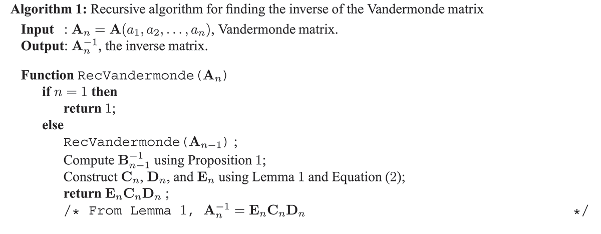
Figure 1. Comparison between the running times of the proposed algorithm and the matrix inversion function in MATLAB. The size of the Vandermonde matrix increases from 10 to 80, and in each iteration the time required to find the inverse function is computed

We compute the required time for updating the Vandermonde matrix using the proposed algorithm as a function of the size of the matrix. The results are compared with the running time of the function implemented in MATLAB for computing the inverse matrix. For each matrix size, we repeated the experiment 100 times and the average running time was found. The initial size of the Vandermonde matrix is 10 and by adding new entries (observing new data) it gradually increases to 80. For the sake of simplicity, the input elements of a $k\times k$ Vandermonde matrix are assumed to be $1,2,\dots ,k$, i.e., ${\mathbf{A}}_k=\mathbf{A}(1,2,\dots ,k)$. As mentioned before, for finding the polynomial p with degree $n-1$ we need n pairs of observations $(x_i,y_i),i=1,2,\dots ,n$. Since our goal here is to test the performance of the proposed algorithm for finding the inverse of the Vandermonde matrix, we just need the first element of each observation. Figure 1 compares the running times of the proposed algorithm with the MATLAB inverse function for finding the inverse of a Vandermonde matrix as a function of the matrix size. The x-axis in Figure 1 is the size of the Vandermonde matrix, and y-axis is the requires time (second) to find the inverse matrix. It can be observed from Figure 1 that the proposed algorithm is faster than the matrix inversion function in MATLAB. ⁴

4. Conclusion

Computing the inverse of a Vandermonde matrix arises in many applications such as polynomial interpolation, curve fitting, and signal processing. In this paper, we proposed a fast recursive algorithm to find the inverse of a Vandermonde matrix. The proposed algorithm in each iteration uses the new entry and the previous inverse matrix to compute the inverse of the increased size Vandermonde matrix. The proposed algorithm can be implemented as a recursive function to find the inverse of a Vandermonde matrix recursively. The running times of the proposed algorithm to find the inverse of a Vandermonde matrix are compared with the inverse function implemented in MATLAB and the simulation results showed that for a sequential data the proposed algorithm is faster than the inverse function in MATLAB.

Additional information

Funding

The author received no direct funding for this research.

Notes on contributors

Youness Aliyari Ghassabeh

Youness Aliyari Ghassabeh received the BS degree in electrical engineering from the University of Tehran, Tehran, Iran, in 2004, the MS degree from K.N. Toosi University of Technology, Tehran, in 2006, and the PhD degree in mathematics and engineering from Queen’s University, Kingston, ON, Canada, in 2013. He was a postdoctoral fellow at the Toronto Rehabilitation Institute, University Health Network, Toronto, ON between 2013 to 2014. He is currently a manager in Operational Risk Methodology group at Bank of Montreal, Toronto, ON, Canada. His main research interests include machine learning, statistical pattern recognition, probability theory and stochastic processes, image/signal processing, source coding and information theory.

Notes

1 For the sake of simplicity, hereafter we use ${\mathbf{A}}_n$ to refer to an $n\times n$ Vandermonde matrix $\mathbf{A}(a_1,a_2,\dots ,a_n)$.

2 Note that $cof{A}_{n_{ij}}/d,i,j=1,\dots ,n$ is jith element of ${\mathbf{A}}_n^{-1}$ (Horn & Johnson, 1990).

3 We assume that the new entries are added from the left to the Vandermonde matrix. So, for a $2\times 2$ Vandermonde matrix ${\mathbf{A}}_2=\mathbf{A}(a_1,a_2)$, we have ${\mathbf{A}}_1=1$ and ${\mathbf{B}}_1=a_2$. For the general $n\times n$ case, see the Proof of Lemma 1 in Appendix.

4 Note that for the proposed algorithm, the required time for finding the inverse matrix using the previous inverse matrix and the new entry is reported.

5 Otherwise, the determinant of the Vandermonde matrix is zero and the inverse does not exist

Appendix 1

Proof of Lemma 1

Proof

We show that ${\mathbf{E}}_{n+1}{\mathbf{C}}_{n+1}{\mathbf{D}}_{n+1}{\mathbf{A}}_{n+1}={\mathbf{I}}_{n+1}$, where ${\mathbf{I}}_{n+1}$ is a $(n+1)\times (n+1)$ identity matrix. To achieve this goal, we start by computing the product of ${\mathbf{D}}_{n+1}$ and ${\mathbf{A}}_{n+1}$,$$\begin{array}{c}\hfill {\mathbf{D}}_{n+1}{\mathbf{A}}_{n+1}=\left(\begin{array}{ccc}1\hfill & 0\dots \hfill & 0\hfill \\ 0\hfill & \hfill & \\ ⋮\hfill & {\mathbf{B}}_n^{-1}\hfill & \\ 0\hfill & \hfill \end{array}\right)\left(\begin{array}{ccccc}1\hfill & 1\hfill & 1\hfill & \dots \hfill & 1\hfill \\ a_{n+1}\hfill & a_1\hfill & a_2\hfill & \dots \hfill & a_n\hfill \\ ⋮\hfill & ⋮\hfill & ⋮\hfill & \dots \hfill & ⋮\hfill \\ a_{n+1}^n\hfill & a_1^n\hfill & a_2^n\hfill & \dots \hfill & a_n^n\hfill \end{array}\right).\end{array}$$

It is straightforward to show that$$\begin{array}{c}\hfill {\mathbf{D}}_{n+1}{\mathbf{A}}_{n+1}=\left(\begin{array}{ccccc}1\hfill & 1\hfill & 1\hfill & \dots \hfill & 1\hfill \\ a_{11}\hfill & 1\hfill & 0\hfill & \dots \hfill & 0\hfill \\ a_{21}\hfill & 0\hfill & 1\hfill & \dots \hfill & 0\hfill \\ ⋮\hfill & ⋮\hfill & ⋮\hfill & \dots \hfill & ⋮\hfill \\ a_{n1}\hfill & 0\hfill & 0\hfill & \dots \hfill & 1\hfill \end{array}\right)=\left(\begin{array}{ccccc}1\hfill & 1\hfill & 1\hfill & \dots \hfill & 1\hfill \\ a_{11}\hfill & \hfill & \hfill & \\ a_{21}\hfill & \hfill & \hfill & \\ ⋮\hfill & {\mathbf{I}}_n\hfill & \hfill & \\ a_{n1}\hfill & \hfill & \hfill & \hfill \end{array}\right),\end{array}$$

where(A1) $$\begin{array}{c}\hfill \left\{\begin{array}{c}{a}_{11}=b_{11}{a}_{n+1}+b_{12}{a}_{n+1}^2+\dots +b_{1n}{a}_{n+1}^n,\hfill \\ a_{21}=b_{21}{a}_{n+1}+b_{22}{a}_{n+1}^2+\dots +b_{2n}{a}_{n+1}^n,\hfill \\ ⋮=⋮\hfill \\ a_{n1}=b_{n1}{a}_{n+1}+b_{n2}{a}_{n+1}^2+\dots +b_{nn}{a}_{n+1}^n.\hfill \end{array}\right.\end{array}$$(A1)

The above equations can be written in the following compact matrix form(A2) $$\begin{array}{c}\hfill \left(\begin{array}{c}{a}_{11}\hfill \\ a_{21}\hfill \\ ⋮\hfill \\ a_{n1}\hfill \end{array}\right)={\mathbf{B}}_n^{-1}\left(\begin{array}{c}{a}_{n+1}\hfill \\ a_{n+1}^2\hfill \\ ⋮\hfill \\ a_{n+1}^n\hfill \end{array}\right).\end{array}$$(A2)

Now, we evaluate ${\mathbf{C}}_{n+1}{\mathbf{D}}_{n+1}{\mathbf{A}}_{n+1}$,$$\begin{array}{c}\hfill {\mathbf{C}}_{n+1}{\mathbf{D}}_{n+1}{\mathbf{A}}_{n+1}=\left(\begin{array}{ccccccc}1\hfill & -1\hfill & -1\hfill & -1\hfill & \dots \hfill & -1\hfill & -1\hfill \\ -1\hfill & 2\hfill & 1\hfill & 1\hfill & \dots \hfill & 1\hfill & 1\hfill \\ -1\hfill & 1\hfill & 2\hfill & 1\hfill & \dots \hfill & 1\hfill & 1\hfill \\ ⋮\hfill & ⋮\hfill & ⋮\hfill & \dots \hfill & ⋮\hfill & ⋮\hfill \\ -1\hfill & 1\hfill & 1\hfill & 1\hfill & \dots \hfill & 1\hfill & 2\hfill \end{array}\right)\left(\begin{array}{ccccc}1\hfill & 1\hfill & 1\hfill & \dots \hfill & 1\hfill \\ a_{11}\hfill & 1\hfill & 0\hfill & \dots \hfill & 0\hfill \\ a_{21}\hfill & 0\hfill & 1\hfill & \dots \hfill & 0\hfill \\ ⋮\hfill & ⋮\hfill & ⋮\hfill & \dots \hfill & ⋮\hfill \\ a_{n1}\hfill & 0\hfill & 0\hfill & \dots \hfill & 1\hfill \end{array}\right).\end{array}$$

It is simple to show that(A3) $$\begin{array}{c}\hfill {\mathbf{C}}_{n+1}{\mathbf{D}}_{n+1}{\mathbf{A}}_{n+1}=\left(\begin{array}{cccccc}{c}_1\hfill & 0\hfill & 0\hfill & \dots \hfill & 0\hfill & 0\hfill \\ c_2\hfill & 1\hfill & 0\hfill & \dots \hfill & 0\hfill & 0\hfill \\ c_3\hfill & 0\hfill & 1\hfill & \dots \hfill & 0\hfill & 0\hfill \\ ⋮\hfill & ⋮\hfill & \dots \hfill & ⋮\hfill & ⋮\hfill \\ c_n\hfill & 0\hfill & 0\hfill & \dots \hfill & 1\hfill & 0\hfill \\ c_{n+1}\hfill & 0\hfill & 0\hfill & \dots \hfill & 0\hfill & 1\hfill \end{array}\right)=\left(\begin{array}{ccc}{c}_1\hfill & 0\dots \hfill & 0\hfill \\ c_2\hfill & \hfill & \\ ⋮\hfill & {\mathbf{I}}_n\hfill & \\ c_{n+1}\hfill & \hfill \end{array}\right),\end{array}$$(A3)

where(A4) $$\begin{array}{cc}& c_1=1-a_{11}-a_{21}-a_{31}\cdots -a_{n1},\hfill \end{array}$$(A4) (A5) $$\begin{array}{cc}& \left\{\begin{array}{c}{c}_2=-1+2a_{11}+a_{21}+a_{31}\cdots a_{n1}=a_{11}-c_1,\hfill \\ c_3=-1+a_{11}+2a_{21}+a_{31}\cdots a_{n1}=a_{21}-c_1,\hfill \\ c_4=-1+a_{11}+a_{21}+2a_{31}\cdots a_{n1}=a_{31}-c_1,\hfill \\ ⋮=⋮=⋮\hfill \\ c_{n+1}=-1+a_{11}+a_{21}+a_{31}\cdots 2a_{n1}=a_{n1}-c_1.\hfill \end{array}\right.\hfill \end{array}$$(A5)

The above equalities can be written in the following matrix(A6) $$\begin{array}{c}\hfill \left(\begin{array}{c}{c}_2\hfill \\ c_3\hfill \\ ⋮\hfill \\ c_{n+1}\hfill \end{array}\right)=\left(\begin{array}{c}{a}_{11}\hfill \\ a_{21}\hfill \\ ⋮\hfill \\ a_{n1}\hfill \end{array}\right)-c_1\left(\begin{array}{c}1\hfill \\ 1\hfill \\ ⋮\hfill \\ 1\hfill \end{array}\right).\end{array}$$(A6)

It remains to show that ${\mathbf{E}}_{n+1}{\mathbf{C}}_{n+1}{\mathbf{D}}_{n+1}{\mathbf{A}}_{n+1}={\mathbf{I}}_{n+1}$. Using Equation (8), we obtain(A7) $$\begin{array}{c}\hfill {\mathbf{E}}_{n+1}{\mathbf{C}}_{n+1}{\mathbf{D}}_{n+1}{\mathbf{A}}_{n+1}=\underset{{\mathbf{E}}_{n+1}}{\underbrace{\left(\begin{array}{ccc}\frac{1}{c_1}\hfill & 0\dots \hfill & 0\hfill \\ \frac{-c_2}{c1}\hfill & \hfill & \\ \frac{-c_3}{c1}\hfill & \hfill & \\ ⋮\hfill & {\mathbf{I}}_n\hfill & \\ \frac{-c_{n+1}}{c_1}\hfill & \hfill \end{array}\right)}}\underset{{\mathbf{C}}_{n+1}{\mathbf{D}}_{n+1}{\mathbf{A}}_{n+1}}{\underbrace{\left(\begin{array}{ccc}{c}_1\hfill & 0\dots \hfill & 0\hfill \\ c_2\hfill & \hfill & \\ ⋮\hfill & {\mathbf{I}}_n\hfill & \\ c_{n+1}\hfill & \hfill \end{array}\right)}}={\mathbf{I}}_{n+1}.\end{array}$$(A7)

Therefore,$$\begin{array}{c}\hfill {\mathbf{E}}_{n+1}{\mathbf{C}}_{n+1}{\mathbf{D}}_{n+1}={\mathbf{A}}_{n+1}^{-1}.\end{array}$$ $\square$

Appendix 2

Proof of Lemma 2

Proof

We use contradiction to show $c_1\ne 0$. Assume the coefficient $c_1$ is zero, i.e. $c_1=0$. Then using Equations (1) and (2), we have(B1) $$\begin{array}{cc}& a_{11}+a_{21}+\dots +a_{n1}=1\hfill \end{array}$$(B1) (B2) $$\begin{array}{cc}& {\mathbf{B}}_n\left(\begin{array}{c}{a}_{11}\hfill \\ a_{21}\hfill \\ ⋮\hfill \\ a_{n1}\hfill \end{array}\right)=\left(\begin{array}{c}{a}_{n+1}\hfill \\ a_{n+1}^2\hfill \\ ⋮\hfill \\ a_{n+1}^n\hfill \end{array}\right).\hfill \end{array}$$(B2)

By combining Equations (9) and (10), we obtain(B3) $$\begin{array}{c}\hfill \left(\begin{array}{ccccc}1\hfill & 1\hfill & \dots \hfill & 1\hfill & 1\hfill \\ a_1\hfill & a_2\hfill & \dots \hfill & a_n\hfill & a_{n+1}\hfill \\ a_1^2\hfill & a_2^2\hfill & \dots \hfill & a_n^2\hfill & a_{n+1}^2\hfill \\ ⋮\hfill & ⋮\hfill & \dots \hfill & ⋮\hfill & ⋮\hfill \\ a_1^n\hfill & a_2^n\hfill & \dots \hfill & a_n^n\hfill & a_{n+1}^n\hfill \end{array}\right)\left(\begin{array}{c}{a}_{11}\hfill \\ a_{21}\hfill \\ ⋮\hfill \\ a_{n1}\hfill \\ -1\hfill \end{array}\right)=\left(\begin{array}{c}0\hfill \\ 0\hfill \\ ⋮\hfill \\ 0\hfill \\ 0\hfill \end{array}\right).\end{array}$$(B3)

The first matrix in (15) is a $(n+1)\times (n+1)$ Vandermonde matrix ${\mathbf{A}}_{n+1}$. Since $a_i,i=1,\dots ,n+1$ are distinct, ⁵ therefore ${\mathbf{A}}_{n+1}$ is a nonsingular matrix and its inverse exists. By multiplying both sides of Equation (15) by ${\mathbf{A}}_{n+1}^{-1}$, we obtain(B4) $$\begin{array}{c}\hfill \left(\begin{array}{c}{a}_{11}\hfill \\ a_{21}\hfill \\ ⋮\hfill \\ a_{n1}\hfill \\ -1\hfill \end{array}\right)=\left(\begin{array}{c}0\hfill \\ 0\hfill \\ ⋮\hfill \\ 0\hfill \\ 0\hfill \end{array}\right).\end{array}$$(B4)

The above equality implies that our assumption, $c_1=0$, is not correct. Therefore, $c_1\ne 0$. $\square$

References

- Aliyari Ghassabeh, Y. , & Abrishami Moghaddam, H. (2013). Adaptive linear discriminant analysis for online feature extraction. Machine Vision Applications , 24 , 777–794.
- Aliyari Ghassabeh, Y. , Rudzicz, F. , & Abrishami Moghaddam, H. (2015). Fast incremental LDA feature extraction. Pattern Recognition , 31 , 1999–2012.
- Barker, H. A. , Tan, A. H. , & Godfrey, K. R. (2004). Optimal levels of perturbation signals for nonlinear system identification. IEEE Transactions on Automatic Conrol , 49 , 1404–1407.
- El-Mikkawya, M. E. A. (2003). Inversion of a generalized Vandermonde matrix. International Journal of Computer Mathematics , 80 , 759–765.
- Eisinberg, A. , & Fedele, G. (2006). On the inversion of the Vandermonde matrix. Applied Mathematics and Computation , 174 , 1384–1397.
- Gautschi, W. , & Inglese, G. (1988). Lower bounds for the condition number of Vandermonde matrix. Numerische Mathematik , 52 , 241–250.
- Gohberg, I. , & Olshevsky, V. (1997). The fast generalized Parker--Traub algorithm for inversion of Vandermonde and related matrices. Journal of Complexity , 13 , 208–234.
- Horn, R. A. , & Johnson, C. R. (1990). Matrix analysis . Cambridge: Cambridge University Press.
- Kaufman, I. (1969). The inversion of the Vandermonde matrix and transformation to the Jordan canonical form. IEEE Transactions on Automatic Control , 14 , 774–777.
- Mirsky, L. (2011). An introduction to linear algebra . New York, NY: Dover Publications.
- Neagoe, V. (1996). Inversion of the Van der Monde matrix. IEEE Signal Processing Letters , 3 , 119–120.
- Olkkonen, H. , & Olkkonen, J. T. (2010). Sampling and reconstruction of transient signals by parallel exponential filters. IEEE Transactions on Circuits and Systems - Part II: Express Briefs , 57 , 426–429.
- Phillips, G. M. (2003). Interpolation and approximation by polynomials . New York, NY: Springer Verlag.
- Ryan, O. , & Debbah, M. (2009). Asymptotic behaviour of random Vandermonde matrices with entries on the unit circle. IEEE Transaction on Information Theory , 55 , 3115–3147.
- Respondek, J. S. (2016). Incremental numerical recipes for the high efficient inversion of the confluent Vandermonde matrices. Computers & Mathematics with Applications , 71 , 489–502.
- Wertz, H. (1965). On the numerical inversion of a recurrent problem: The Vandermonde matrix. IEEE Transactions on Automatic Control , 10 , 492.
- Wang, Z. , Scaglione, A. , Giannakis, G. , & Barbarossa, S. (1999). Vandermonde--Lagrange mutually orthogonal flexible transceivers for blind CDMA in unknown multipath. In Proceedings of 2nd IEEE Workshop on Signal Processing Advances in Wireless Communications (pp. 42–45). Minneapolis, MN.
- Wilf, H. S. (1958). Curve-fitting matrices. The American Mathematical Monthly , 65 , 272–274.
- Tou, J. (1964). Determination of the inverse Vandermonde matrix. IEEE Transactions on Automatic Control , 9 , 314.