Identification and control of an oxygen provider system for a biological capsule

Abstract

Providing oxygen is a necessary process in manned missions to space. The aim of this paper is to identify the dynamics of an open loop control system in preparation for feature missions. A linear time invariant model is identified with data gathered from pre-flight tests of Kavoshgar, the Iranian bio-capsule. Numerical evaluation of the resulting model and its validation are given. The resulting time discrete model is used to drive the optimal setting that minimizes power consumption of the system.

Keywords:

• system identification
• control
• parameter estimation
• power minimization
• linear time invariant systems

Public Interest Statement

This research is the first attempt to find a mathematical model for an oxygen provider system in a biological capsule. Using experimental data and methods of system identification, the relations between different environmental parameters of the capsule were formulated as a valid discrete linear dynamical system. Optimal control for minimizing the electrical power consumption was also studied. The results and methods may be used to increase the level of automation of the next generation of the biological capsules.

1. Introduction

Reduction of ${\text{CO}}_2$ and providing oxygen is one of the most important considerations in a manned flight to outer space. Controlling the levels of gases in a closed, sealed area with limitations of weight, power, and volume, and their impact on the health of the crew, define our special technical and operational requirements. In addition to transferring oxygen with bio-capsules from earth, there are oxygen releasing systems based on the electrolysis of silicate melt (Colson & Haskin, 1993), the photosynthetic gas exchanger (Bates, 1961), the carbothermal process (Cutler & Krag, 1985), and oxygen-organic materials (Kaoa, Chen, & Suc, 2001).

To provide the required oxygen, and eliminate ${\text{CO}}_2$ exhaled by the monkey, an oxygen provider system (OPS) was designed for Kavoshgar, which is a manned space vehicle carrying a rhesus monkey into suborbital flight. This gas-controlling system works based on chemical reactions. In past missions, the oxygen provider was powered on continuously for the entire 5 h mission for safety and to avoid hypoxia. Owing to previous success and increased levels of technological readiness, there is interest in being able to control the oxygen levels by powering the system on and off during the mission, and during special situations. This will result in a reduction of power consumption, weight, cost of materials, and provide better living conditions.

In order to design such a controller, the dynamics of the system are required as the first step. The impact of the on/off switching on the current and feature levels of gases has to be known. This motivates our system identification approach to be able to estimate the system behavior via experimental data gathered during integration and final tests.

For some of the recent application of system identification, for example, Zhang, Wei, and Qi (2016) may be addressed, where, a recursive least-squares algorithm was used for online parameter identification and estimation of the amount of charge in lithium iron phosphate batteries. In Delpoux and Floquet (2015), an algebraic online parameter estimation method was proposed and applied to a permanent magnet stepper motor. A new class of non-linear fractional models based on the Volterra series was proposed by Maachoua et al. (2014) for modeling non-linear diffusive phenomena in order to estimate thermal parameters in cases where the temperature variations are large. In Wang (2015), a fast affine projection technique was applied for system identification of a DC–DC convertor in order to drive a novel adaptive control technique for the output voltage regulation of the convertor, and to improve its dynamic response.

In the present work, a linear time variant model is determined to simulate the system response. The resulting system is marginally stable, and simulations show reasonable accuracy of the model. The model is also evaluated and validated with data-sets.

Finally, the optimal control of the resulting time discrete system is studied. The problem of optimal control leads to solving a linear programming problem with binary variables. Examining the optimal solution in test cases confirms the desired reduction in power consumption.

2. System description

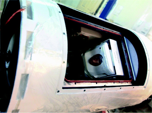
One of the most important aspects of space missions for Kavoshgar is to investigate biological treatments and to develop life support systems for future projects. For this purpose, a biological capsule was designed to accommodate a rhesus monkey (Figure 1). This module contained life support equipments such as monitoring vital signals, isolation, seat, and an OPS.

Figure 1. Biological capsule.

Obviously, any living being onboard the spacecraft consumes oxygen and produces ${\text{CO}}_2$. For a 4 kg rhesus monkey, according to Bourne (1975), the rate of oxygen consumption is $51.7\pm 10.3$ ml/min. In our test case, the ${\text{CO}}_2$ concentration when the monkey is in the biological capsule with closed doors grows from 400 to 6,000 ppm in 15 min when the oxygen provider system is off. This means that, the ${\text{CO}}_2$ production rate in an 80 L volume of the pressurized capsule is 29.86 ml/min. According to Rising and Lin (2013), the respiratory quotient of the rhesus monkey in an unstressed situation is 0.75. Then, the oxygen consumption rate for the monkey in the experimental test is 39.81 ml/min, which is in the theoretical range.

The aforementioned calculations show that a monkey consumes oxygen in its closed area at a rate of about 40 ml/min. Remembering the 5 h total mission time, 72 L of oxygen is needed, which is impossible to include from the mission onset: the capacity of the bio-capsule is 80 L, where the maximum fraction of initial oxygen can only be 25% of the total volume. This shows the existence of a system for ${\text{CO}}_2$ reduction and oxygen production is an essential requirement. To meet this requirement, a chemical reactor was developed for Kavoshgar project. It works based on the following chemical reaction, where sodium peroxide reacts with ${\text{CO}}_2$ to produce oxygen:(1) $$\begin{array}{c}\hfill {\text{Na}}_2{\text{O}}_2+{\text{CO}}_2\to {\text{Na}}_2{\text{O}}_3+\frac{1}{2}{\text{O}}_2\end{array}$$(1)

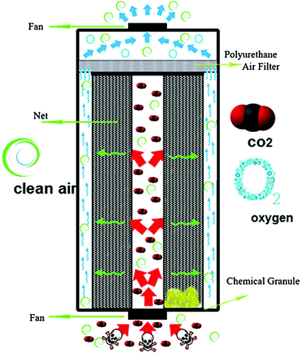
With this reaction, the ${\text{CO}}_2$ produced by respiration reacts with ${\text{Na}}_2{\text{O}}_2$ to make oxygen. As depicted in Figure 2, the system consists of three hollow cylinders. A fan in the bottom pulls air into the central cylinder. Then, air enters into the second part which is a porous medium filled with ${\text{Na}}_2{\text{O}}_2$ granules. The chemical reaction (1) occurs in this section, and the clean air is withdrawn by the upper fan and enters back into the bio-capsule.

Figure 2. Schematic of the OPS. Source: Javadi, Zakeri, Salimi, Sheyda, and Ebrahimi (2013).

3. Experimental setup

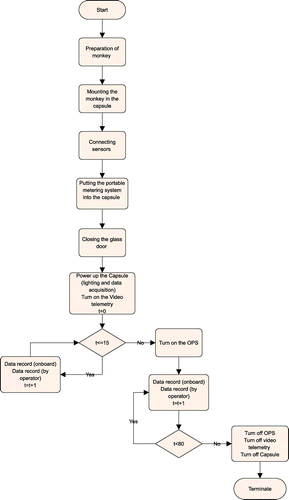
In order to gather data and identify the influencing factors of the capsule’s environment, a series of test was performed. In these preflight tests, the monkey was in a sealed capsule similar to real flight conditions. All instruments and sensors were attached to the monkey and the capsule. Then, the onboard data-gathering system was powered up and recorded the environmental parameters and vital signals at a rate of one sample per minute. Data were also recorded by operators from portable metering devices in order to check the acquisition system. Table 1 shows the equipment which were used in this test.

Table 1. Equipment and their tasks in the experimental test

Equipment	Task
Biological capsule	Providing the space for sitting the monkey, supplying the internal lighting
Oxygen providing system	Reduction of ${\text{CO}}_2$, providing oxygen for the monkey, air conditioning
Power unit	Supplying electrical power for the operation of the OPS, lighting system, and onboard data acquisition
Video telemetry	Sending online pictures of the monkey’s situation for monitoring in the ground station
Onboard data acquisition	Sampling and recording data from the environmental and vital sensors
Portable metering device	Indication environmental and vital signals such as internal pressure, temperature, humidity, ${\text{CO}}_2$ and oxygen concentration
Onboard environmental sensors	Measuring the internal temperature, internal pressure (two sets), air humidity, ${\text{CO}}_2$ concentration, and oxygen concentration
Vital sensors	Measuring the heart rate, skin temperature, and tympanic temperature

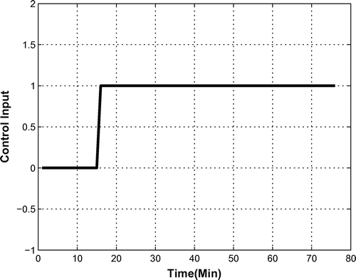
In the first part of the sampling process, the OPS was off for the first 15 min and turned on for the remaining 65 min of the test. Data were gathered as is shown and studied in Section 4. Figure 3 shows a flowchart of the test process.

Figure 3. Flowchart of the experimental test for gathering the required data.

4. Environmental factors

In past missions, the system is powered on 30 min before launch up to the end of the mission (5 h). Test results show that the system is not necessarily working, and hence turned on, over the entire duration of the mission; indeed, it may be powered on and off in special circumstances. In order to find such time points, knowledge of the dynamics and characteristics of the system is required. The important environmental parameters are listed subsequently.

4.1. Oxygen

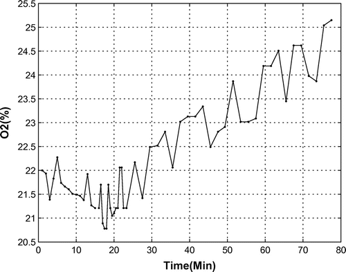
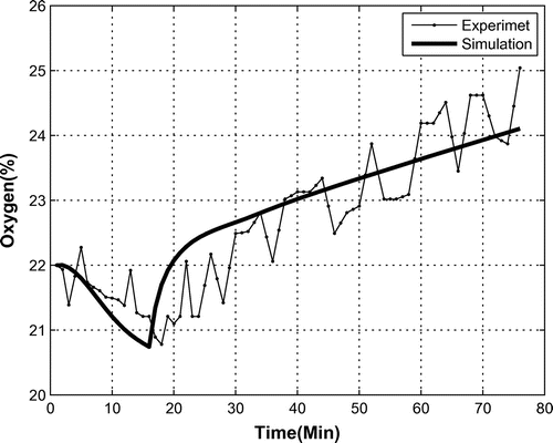
A correctly operating OPS increases the percentage of oxygen in the bio-capsule. In a functional system test with a monkey in its seat and with closed doors, the OPS is first turned off for 15 min, whereby it is turned on to measure the amount oxygen and ${\text{CO}}_2$ changes. During this test, data from onboard sensors was recorded every minute as shown in Figure 4. In the first part, i.e. without oxygen production, the oxygen levels decreased from 22 to 21% because of the monkey’s breathing. After turning on the OPS, oxygen was produced and its percentage increased up to 25% at the end of the first hour of OPS operation. As oxygen levels over 25% are harmful for the creature, is it necessary to power off the OPS at some time based on knowledge of the system’s dynamics, which will be determined via system identification.

Figure 4. Oxygen percentage in the bio-capsule.

4.2. Carbon dioxide

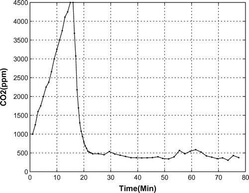
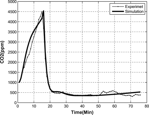
In the aforementioned experimental test, the amount of ${\text{CO}}_2$ was also measured, see Figure 5. As can be seen, up to the 15th minute of the test, i.e. when the OPS was turned off, the density of ${\text{CO}}_2$ increased due to the animal’s breathing. When oxygen production started, the amount of ${\text{CO}}_2$ decreased based on reaction (1). In a 1 h test, the ${\text{CO}}_2$ amount decreased from 4,500 to 380 ppm.

Figure 5. Carbon dioxide density in the bio-capsule.

Figure 6. Internal temperature in the bio-capsule.

4.3. Temperature

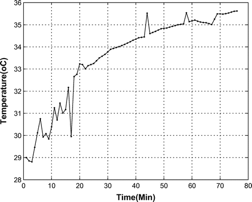
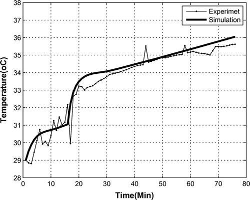
The reaction (1) is exothermic and adds heat to the bio-capsule. As is shown in Figure 6, during a 80 min mission, the temperature increased from 29 to 35.5${}^{\circ }$C. Therefore, based on the linear behavior of temperature, for a full mission, an increase of about 24${}^{\circ }$C is expected, which may be harmful for the monkey when the oxygen provider is working all the time and when finding the payload takes a long time.

It should be noted that there are other heat sources, such as the monkey itself, electrical equipment in the capsule, and lighting. However, the quota of the oxygen provider is considerable, and designers are interested in identifying the relationship between the temperature changes caused by the OPS and other parameters via the experimental data used in this paper.

4.4. Pressure

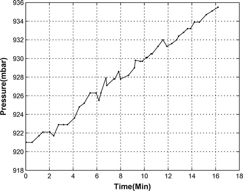
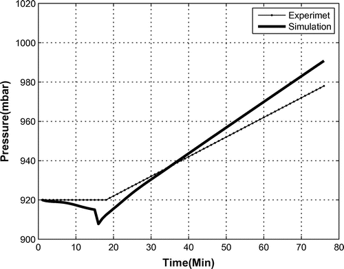
Internal pressure of the bio-capsule is another key parameter affected by the operating OPS. As shown in Figure 7, the process of converting ${\text{CO}}_2$ to oxygen increases the internal pressure. In our test case, the pressure grew from 920 to 936 millibar in 16 min. This shows that the pressure increases 1 millibar per minute when the OPS is working continuously.

Figure 7. Internal pressure of the bio-capsule.

4.5. Humidity

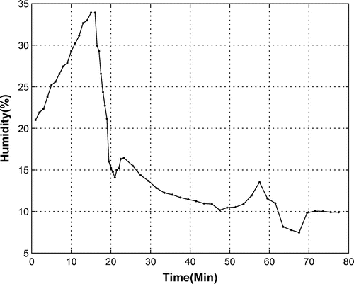
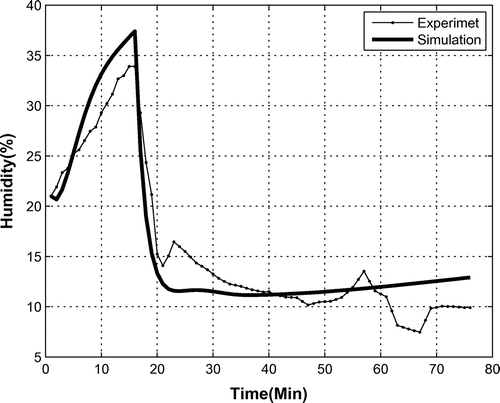
The exothermic behavior of reaction (1) causes a reduction of humidity in the bio-capsule, while the respiration of the monkey increases it. However, the drying attributed to the oxygen provider overcomes the effect of respiration to the overall humidity. Figure 8 shows the percentage of humidity in an experimental test. In this test, the OPS was powered off from begin up to 15 min, then it was powered on for 1 h. Results show that the humidity increased from 21 to 34% when the OPS was switched off. This increase was due to the respiration of the animal. When the OPS was powered on, the humidity decreased as expected, from 33 to 8%. During this phase, the dominancy of the OSP to the monkey respiration toward air-drying is proved. It is clear that when the mission takes a long time, the humidity in the bio-capsule drops. It should be noted that humidity is also influenced by temperature, the amount of ${\text{CO}}_2$ and oxygen in the air, and the internal pressure.

Figure 8. Humidity levels in the bio-capsule.

4.6. Correlations

A quick view of the aforementioned graphs (Figures 4–8) indicates that there are some relationships and dependencies between the related parameters. The internal temperature and pressure, for example, seem to increase at the same rate. Humidity and ${\text{CO}}_2$ both decrease, and it seems that they are correlated with each other. To illustrate the quantitative measure of such dependencies, one may use the cross-correlation coefficient between each pairs of experimental data, which is defined as:(2) $$\begin{array}{c}\hfill R(x,y)=\frac{{\sum }_{i=0}^N(x_i-\overline{x})(y_i-\overline{y})}{\sqrt{\sum _{i=0}^N{(x_i-\overline{x})}^2\sum _{i=0}^N{(y_i-\overline{y})}^2}}\end{array}$$(2)

where $\overline{x}$ stands for the average of x. The cross-correlation coefficient ranges from $-1.0$ to $+1.0$. A value of $-1.0$ indicates a perfect negative correlation, while a correlation of 1.0 indicates a perfect positive correlation. Some of the cross-correlation for the related data were calculated, for example:

$R(\text{oxygen},{\text{CO}}_2)=-0.55$

$R(\text{oxygen},\text{Humidity})=-0.71$

$R(\text{oxygen},\text{Temperature})=0.70$

$R({\text{CO}}_2,\text{Humidity})=0.95$

$R({\text{CO}}_2,Temperature)=-0.67$

$R(\text{Humidity},\text{Temperature})=-0.82$

This shows that, for the above example, the ${\text{CO}}_2$ density and humidity percentage are highly correlated with each other, while the humidity and temperature are negatively correlated with each other. This shows the dependency of these quantities within the closed environment of the bio-capsule. A mathematical model that describes hidden relations in this system via mathematical expressions is presented in Section 5.

5. System identification

As mentioned previously, a system identification method was used to describe the dynamics of the OPS as mathematical relations. First, the input and output signals are defined. Let us assume that u(t) is the on–off situation of the OPS at time t, which is considered as the input of the system. It is a Bang–Bang control with 0–1 values as:(3) $$\begin{array}{c}\hfill u(t)=\left\{\begin{array}{cc}1\hfill & \text{if the OPS is on at time}t,\hfill \\ 0\hfill & \text{if the OPS is off at time}t.\hfill \end{array}\right.\end{array}$$(3)

There are five components of the output vector:(4) $$\begin{array}{c}\hfill y(t)={(y_1(t),y_2(t),y_3(t),y_4(t),y_5(t))}^T\end{array}$$(4)

as follows:

$y_1(t)=$ Percentage of oxygen in the capsule

$y_2(t)=$ Carbon dioxide density in the capsule (ppm)

$y_3(t)=$ Percentage of humidity in the capsule

$y_4(t)=$ Temperature in the capsule (${}^{\circ }$C)

$y_5(t)=$ Internal pressure in the capsule (millibar)

Figure 9. Input signal used in the identification process.

For the model set, let us consider a set of discrete time invariant linear state space systems as:(5) $$\begin{array}{cc}& x(t+1)=Ax(t)+Bu(t)\hfill \end{array}$$(5) (6) $$\begin{array}{cc}& y(t)=Cx(t)+Du(t)\hfill \end{array}$$(6)

With a degree of 5, there are 60 unknown coefficients in matrices A, B, C, and D which have to be determined in such a way that the resulting system estimate matches the experimental data. Data were gathered when the OPS was off for 15 min, and then turned on for 60 min. As such, the response of the system to a step input, as in Figure 9, is available for identification. The parameter estimation method (Ljung, 1999) was used to find the model parameters. It is assumed that vector Z shows all experimental data, and $\mathit{\theta }$ shows all unknown parameters. The related error of an individual parameter $\mathit{\theta }$ is defined as:(7) $$\begin{array}{c}\hfill \mathit{\epsilon }(t,\mathit{\theta })=y(t)-\widehat{y}(t),\end{array}$$(7)

where y(t) is the experimental value, and $\widehat{y}(t)$ is its related estimation. In the case of this research, a set of data gathered during an experimental preflight test for $N=80$ min was used. The sampling rate was one sample per minute. In addition to recording the sensor data with the data acquisition system, samples were checked with an analog thermometer, barometer, and ${\text{CO}}_2$ indicator. Therefore, with 80 samples in each of the five channels in (4), the vector $Z=[y(t_0),y(t_1),\dots ,y(t_{79})]$ is ready. Then, the vector of parameters ${\mathit{\theta }}^{\ast }$ has to be determined in such a way that $\mathit{\epsilon }(t_i,\mathit{\theta })$ in (7) is zero for all samples. However, with 60 unknown parameters and 80 equations, this is an over-determined linear system. An efficient method for solving such a system is to use the least-squares method in which the following average norm of errors has to be minimized:(8) $$\begin{array}{c}\hfill V_N(\mathit{\theta },Z)=\frac{1}{N}\sum _{i=1}^N{(\mathit{\epsilon }(t_i,\mathit{\theta }))}^2.\end{array}$$(8)

The total error function of (8) was minimized using the least-squares method proposed in Farahi, Fahimian, and Nazemi (2008). The matrix coefficients were found as:$$\begin{array}{cc}& A=\left[\begin{array}{ccccc}0.5089\hfill & 0.2913\hfill & -0.2753\hfill & -0.0322\hfill & 0.1015\hfill \\ -0.0048\hfill & 0.9675\hfill & -0.0843\hfill & -0.0213\hfill & -0.0178\hfill \\ -1.1719\hfill & -0.2220\hfill & 0.7467\hfill & -0.0389\hfill & 0.0415\hfill \\ 0.1790\hfill & 0.2837\hfill & -0.0181\hfill & 0.7921\hfill & 0.3327\hfill \\ 0.06241\hfill & -0.2489\hfill & -1.003\hfill & -0.3743\hfill & 0.9305\hfill \end{array}\right]\hfill \\ \hfill & B={\left[\begin{array}{ccccc}-0.8966\hfill & -0.6064\hfill & -0.3525\hfill & -0.2185\hfill & -0.7204\hfill \end{array}\right]}^T\hfill \\ \hfill & C=\left[\begin{array}{ccccc}-1.888\hfill & 51.69\hfill & 0.3654\hfill & 2.468\hfill & -3.865\hfill \\ 3154\hfill & 3505\hfill & -1191\hfill & 6.615\hfill & -606.8\hfill \\ 20.61\hfill & 45.30\hfill & -8.38\hfill & 0.3182\hfill & -7.399\hfill \\ -2.048\hfill & 70.38\hfill & -2.07\hfill & 3.22\hfill & -4.921\hfill \\ -24.77\hfill & 2131\hfill & -29.46\hfill & 91.96\hfill & -166.4\hfill \end{array}\right]\hfill \\ \hfill & D={\left[\begin{array}{ccccc}0\hfill & 250\hfill & 0\hfill & 0\hfill & -7\hfill \end{array}\right]}^T\hfill \end{array}$$

5.1. Stability

To study the stability properties of the resulting linear time invariant system, the magnitude of the eigenvalues of matrix A were calculated, and found to be 1.0001, 0.9241, 0.8231, 0.8231, 0.5120. Since these eigenvalues are in the unit circle or on its boundary, the system is marginally stable (Boom, 2006). This means that if an impulse of finite magnitude is given as input, then the system will not give an unbounded output, but neither will the output return to zero.

5.2. Validation

To check the validity of our results, the estimation was calculated using the input signal of the experiment and comparing the estimated and actual data. To start the simulation, initial parameter values are needed. From the experimental data, $y(0)={(22,1000,21,29,920)}^T$. Therefore, the related initial value for the state vector was calculated as:$$\begin{array}{c}\hfill x(0)=C^{-1}(y(0)-Du(0))=\left[\begin{array}{c}-0.1674\hfill \\ 0.5431\hfill \\ 0.4492\hfill \\ -3.7682\hfill \\ -0.7110\hfill \end{array}\right]\end{array}$$

Figure 10. Experimental and simulated data oxygen percentages.

In Figure 10, the simulated oxygen percentage is shown. It is clear that the simulated output of the resulting system tracks the data well.

A similar graph of the ${\text{CO}}_2$ density is also depicted in Figure 11. The simulation coincides with the experimental data for the first 20 min, and after that an acceptable trend is observed.

Figure 11. Experimental and simulated ${\text{CO}}_2$ densities.

Figure 12 shows the experimental and estimated humidity in the capsule. As can be seen, the founded model estimates this quantity well.

Figure 12. Experimental and simulated humidity levels.

The model also estimated the temperature and pressure, as can be seen in Figures 13 and 14. For the final course of pressure, the model over-estimates the pressure by 15%, but still maintains the general trend, which has an acceptable accuracy.

Figure 13. Experimental and simulated temperature.

Figure 14. Experimental and simulated pressure.

Figure 15. System responses to $u(t)=0$ and $u(t)=1$.

6. Optimal control

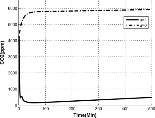
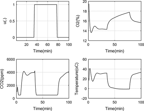
The system response to the two possible step functions $u=0$ and $u=1$ were obtained as depicted in Figure 15. When the OPS was off, the ${\text{CO}}_2$ level reached and stayed at 6,000 ppm, which coincides well with the experimental results.

The aim of the optimal control was to keep the gases and environmental levels at a desired level, while minimizing the power usage by switching the OPS on and off.

It is to be noted that open loop control is preferred to closed loop control because the latter needs to measure the level of gases and environmental factors, where, low reliable sensors, will affect the control loop.

With regards the problem of power and energy minimization, the objective usually has a quadratic form. However, in the present case, as the control values are binary $u(t)\in \{0,1\}$, the quadratic form is equivalent to the linear one. Therefore, the objective function here is considered as a weighed summation of the control values, as follows, in discrete form, which is to be minimized:(9) $$\begin{array}{c}\hfill \sum _{t=0}^{N}r(t)u(t).\end{array}$$(9)

Here, $r(t),t=0,1,2,\dots ,N$ are positive weights. There are also possible constraints on the responses:(10) $$\begin{array}{c}\hfill y_{min}\le y(t)\le y_{max},\end{array}$$(10)

where $y_{min}$ and $y_{max}$ are vectors of the lower and upper limits on the responses of system (5)–(6), respectively. Given an initial value of $x(0)=x_0$, using a procedure similar to the one presented in Goodwin and Seron (2005), and including Equation (5), the state vector $x_t=x(t)$ which is related to the unknown input $u_t=t(u)$ is obtained as:(11) $$\begin{array}{c}\hfill \begin{array}{c}{x}_1=A{x}_0+B{u}_0,\hfill \\ x_2=A^2{x}_0+AB{u}_0+B{u}_1,\hfill \\ ⋮\hfill \\ x_N=A^N{x}_0+A^{N-1}B{u}_0+\cdots +B{u}_{N-1}.\hfill \end{array}\end{array}$$(11)

The aforementioned equation may be written in matrix form as follows:(12) $$\begin{array}{c}\hfill \mathbf{x}=\mathrm{\Gamma }\mathbf{u}+\mathrm{\Omega }{x}_0,\end{array}$$(12)

where,$$\begin{array}{c}\hfill \mathrm{\Gamma }=\left[\begin{array}{cccc}B\hfill & 0\hfill & \cdots \hfill & 0\hfill \\ AB\hfill & B\hfill & \cdots \hfill & 0\hfill \\ ⋮\hfill & ⋮\hfill & ⋮\hfill & ⋮\hfill \\ A^{N-1}B\hfill & A^{N-2}B\hfill & \cdots \hfill & B\hfill \end{array}\right],\mathrm{\Omega }=\left[\begin{array}{c}A\hfill \\ A^2\hfill \\ ⋮\hfill \\ A^N\hfill \end{array}\right],\mathbf{x}=\left[\begin{array}{c}{x}_1\hfill \\ x_2\hfill \\ ⋮\hfill \\ x_N\hfill \end{array}\right],\mathbf{u}=\left[\begin{array}{c}{u}_0\hfill \\ u_1\hfill \\ ⋮\hfill \\ u_{N-1}\hfill \end{array}\right].\end{array}$$

Therefore, from (6) and (12), the vector of the system’s responses is calculated as:(13) $$\begin{array}{c}\hfill \mathbf{y}=(C\mathrm{\Gamma }+\text{diag}(D))\mathbf{u}+C\mathrm{\Omega }{x}_0,\end{array}$$(13)

where $\text{diag}(D)$ is a block diagonal matrix with D as its diagonal entries, and multiplication of C to $\mathrm{\Gamma }$ and $\mathrm{\Omega }$ is performed in a component-wise manner. The constraints may also be written as:(14) $$\begin{array}{c}\hfill \mathbf{y}\le y_{max},-\mathbf{y}\le -y_{min}.\end{array}$$(14)

Now, merging (13) and (14) results in:(15) $$\begin{array}{c}\hfill L\mathbf{u}\le W,\end{array}$$(15)

where,$$\begin{array}{c}\hfill L={\left[\begin{array}{c}(C\mathrm{\Gamma }+\text{diag}(D))\hfill \\ -(C\mathrm{\Gamma }+\text{diag}(D))\hfill \end{array}\right]}_{10N\times N},W={\left[\begin{array}{c}{y}_{max}-C\mathrm{\Omega }{x}_0\hfill \\ -y_{min}+C\mathrm{\Omega }{x}_0\hfill \end{array}\right]}_{10N\times 1}.\end{array}$$

Therefore, the problem of optimally controlling the power consumption is reduced to the following integer linear programming problem with $10N$ constraints:(16) $$\begin{array}{c}\hfill \begin{array}{c}\text{min}\mathbf{r}.\mathbf{u}\hfill \\ \text{s.t.}\hfill \\ L\mathbf{u}\le W\hfill \\ \mathbf{u}\in \{0,1\}\hfill \end{array}\end{array}$$(16)

where $\mathbf{r}=[r(0),r(1),\dots ,r(N-1)]$. The only decision variable in this linear programming problem is vector $\mathbf{u}$ with N components. After solving this problem, the optimal control will be found.

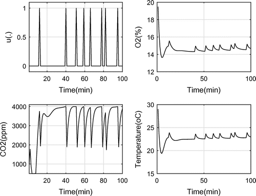
The problem was solved with the branch-and-bound algorithm in $N=100$ min, $r(t)=1,t=0,1,\dots ,N$, and a set of parameters as shown in Table 2. In the first simulation, the upper bound for ${\text{CO}}_2$ is 4,000, the optimal objective function is eight which is 92% lower than the case when the OPS is working continuously during this time period.

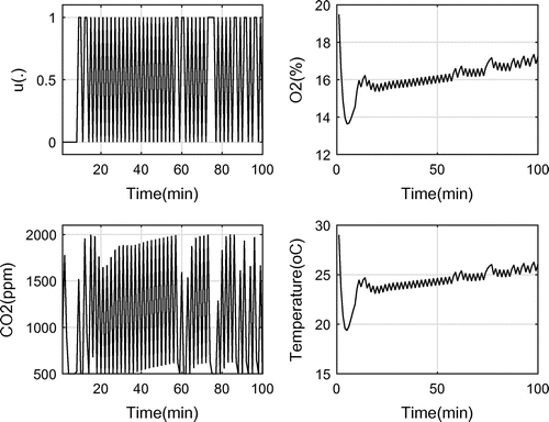
Figure 16 shows the control function, and the system responses to it including ${\text{CO}}_2$ and oxygen levels and temperature. As it can be seen, the resulting optimal control has an off-on-off form with 16 switches between the on and off positions.

Figure 16. The optimal control and system responses for a ${\text{CO}}_2$ upper bound of 4,000 ppm.

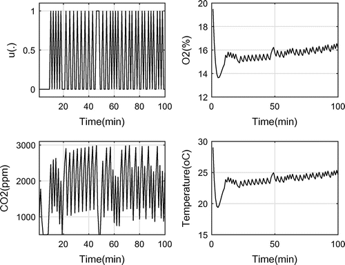
In the second case, the upper bound for ${\text{CO}}_2$ is set to 3,000 ppm, therefore, more working periods of OPS was expected to keep the ${\text{CO}}_2$ level below 3,000 ppm with respect to the first case.

As depicted in Figure 17, the control function has more switches. The optimal objective, as expected, increases to 36 which is 42% lower than full working of OPS. This means that when using the resulting control function, the power consumption reduces by 42%, while the ${\text{CO}}_2$ level does not grow over 3,000 ppm.

Figure 17. The optimal control and system responses for a ${\text{CO}}_2$ upper bound of 3,000 ppm.

In the third run, the upper bound of ${\text{CO}}_2$ was set to 2,000 ppm. The results are shown in Figure 18. The objective reduced to 51 with 100 switches.

Figure 18. The optimal control and system responses for a ${\text{CO}}_2$ upper bound of 2,000 ppm.

Table 2. Best-fitting parameter values

	Oxygen	${\text{CO}}_2$	Humidity	Temperature	Pressure
min	19	500	5	28	870
max	22	2,000, 3,000, 4,000	42	33	905
initial value	22	1,000	16	29	880

6.1. Averaging approach

When solving (16), it was seen that the control function has many switches, especially when the ${\text{CO}}_2$ upper bound decreased. In cases such as a sequence turning on and off what is undesirable, the averaging approach may be applied. In this case, the upper bound on each element of $\mathbf{y}$ is set to the relating average. For example, for ${\text{CO}}_2$, the present constraints in (10) are(17) $$\begin{array}{c}\hfill y_{min}\le y_2(t)\le y_{max},t=1,2,\dots ,N.\end{array}$$(17)

However, in averaging approach, they read as:(18) $$\begin{array}{c}\hfill y_{min}\le {\overline{y}}_2\le y_{max},t=1,2,\dots ,N,\end{array}$$(18)

where,(19) $$\begin{array}{c}\hfill {\overline{y}}_2=\frac{1}{N}\sum _{t=1}^N{y}_2(t).\end{array}$$(19)

Therefore, the linear programming problem (16) is changed to an averaged form as follows:(20) $$\begin{array}{c}\hfill \begin{array}{c}\text{min}\mathbf{r}.\mathbf{u}\hfill \\ \text{s.t.}\hfill \\ \overline{L}\mathbf{u}\le \overline{W}\hfill \\ \mathbf{u}\in \{0,1\}\hfill \end{array}\end{array}$$(20)

Here the number of constraints was reduced to five, and each of them is related to one of the parameters of Table 2.

The problem (20) was also solved for the same values used in the non-averaged method. The results for a ${\text{CO}}_2$ upper bound of 2,000 ppm are shown in Figure 19, for example. It is clear that the control function does not have the same fluctuations as seen in Figure 18 and there are only two switches, while the average ${\text{CO}}_2$ level remained below the upper bound. In order to compare the averaged and non-averaged approaches, in Table 3 the solution parameters are compared. The second column shows the upper bound of ${\text{CO}}_2$, while the third column shows the wall clock time (WCT) that measures the running time for solving the related LP problem. As is expected, because of the reduction in the number of constraints in (20), solving the averaged problem is very fast with respect to the non-averaged method. The number of switches is also reduced to two in all three cases. The objective function and power consumption is also better than in the non-average case. The last column shows the improvement in power consumption with respect to the case of a fully operating OPS.

It should be noted that the solution of the averaged approach will violate the upper and lower bound, but remains in the region in an average meaning.

Figure 19. The optimal control and system responses for a ${\text{CO}}_2$ upper bound of 2,000 ppm (average).

Table 3. Comparison of results

Method	${\text{CO}}_2$ bound	WCT (s)	Switches	Objective	Improvment
Non-average	4,000	221.86	16	8	92%
Non-average	3,000	2,234.27	32	36	64%
Non-average	2,000	2,762.68	100	51	49%
Average	4,000	0.34	2	2	98%
Average	3,000	0.34	2	16	76%
Average	2,000	0.33	2	43	57%

7. Conclusion

A linear time invariant model was obtained to describe the governing dynamics of an OPS for a space bio-capsule. Our chosen parameter estimation method was based on system identification theory. The resulting model was also validated via experimental data. Finally, the model was used to design an open loop controller. Simulations show that with the obtained optimal control, the desired environmental conditions are preserved and electrical power consumption is reduced.

Additional information

Funding

The author received no direct funding for this research.

Notes on contributors

H.H. Mehne

H.H. Mehne was born in Mashhad, Iran, 1978. He received BSc, MSc, and PhD degrees from Fredowsi University of Mashhad, all in Applied Mathematics, in 1999, 2001, and 2005, respectively. Currently, he is an assistant professor at the Aerospace Research Institute (Tehran, Iran). His research interests are optimal control, numerical mathematics, shape optimization, and parallel computing.

References

- Bates, J. H. (1961). Recent aspects in the development of a closed ecologic system. Aerospace Medicine, 32, 12–24).
- Boom, T. (2006). Discrete-time systems analysis. Additional Lecture Notes for the course SC4090. Retrieved from http://www.dcsc.tudelft.nl/~sc4060/transp/discreteNOTES.pdf
- Bourne, G. H. (Ed.). (1975). The Rhesus monkey, Vol I., anatomy and physiology. New York, NY: Academic Press Inc.
- Colson, O. R., & Haskin, L. A. (1993). Producing oxygen by silicate melt electrolysis, resources of near-earth space. J. S. Lewis, M. S. Matthews, & M. L. Guerrieri (Eds.), Space Science Series (pp. 109–127). Tucson, London: The University of Arizona Press.
- Cutler, A. H., & Krag, P. A. (1985). Carbothermal scheme for lunar oxygen production. In W. W. Mendell (ed.), Lunar bases and space activities of the 21st century (pp. 559). Houston, TX: Lunar and Planetary Institute.
- Delpoux, R., & Floquet, T. (2015). On-line parameter estimation via algebraic method: An experimental illustration. Asian Journal of Control, 17, 315–326.
- Farahi, M. H., Fahimian, H., & Nazemi, A. R. (2008). Using least square method to find the approximate solution of an overdetermined system of linear equations. Journal of Mathematical Extension, 2, 113–122.
- Goodwin, G. C., & Seron, M. M. (2005). Constrained control and estimation an optimisation approach. London: Springer.
- Javadi, K. H., Zakeri, R., Salimi, M. R., Sheyda, M., & Ebrahimi, M. (2013). Design and manufacturing of the oxygen provider system of Kavoshgar-6 payload (Technical Report). Aerospace Research Institute. Doc.No.944-91-160
- Kaoa, C. M., Chen, S. C., & Suc, M. C. (2001). Laboratory column studies for evaluating a barrier system for providing oxygen and substrate for TCE biodegradation. Chemosphere, 44, 925–934.
- Ljung, L. (1999). System identification, theory for the user. Englewood Cliffs, NJ: Prentice Hall PTR.
- Maachoua, A., Maltia, R., Melchiora, P., Battagliab, J.-L., Oustaloupa, A., & Hay, B. (2014). Nonlinear thermal system identification using fractional Volterra series. Control Engineering Practice, 29, 50–60.
- Rising, R., & Lin, J. (2013). Low respiratory quotients in chow-fed Male Bonnet Macaque monkeys as a potential indicator of metabolic stress due to single cage housing. Journal of Primatology, 2(2), 1–6.
- Wang, C. (2015). System identification and adaptive control of a DC-DC converter using a current balancing ON/OFF control technique for optimal transient performance. In 17th European Conference on Power Electronics and Applications (EPE’15 ECCE-Europe). Geneva.
- Zhang, J., Wei, Y., & Qi, H. (2016). State of charge estimation of LiFePO4 batteries based on online parameter identification. Applied Mathematical Modelling, 40, 6040–6050.