Demand–supply equilibrium in deregulated electricity markets for future smartgrid

Abstract

Deregulation of electricity market has a potential to improve efficiency, reduce costs for both customers and utilities and improve customer services if implemented correctly. However, it also introduces variability of both demand and supply. For grid stability and reliability, supply and demand must be matched at all times. In this work, the deregulated electricity market has been modeled in a game-theoretic manner as a Potluck problem with non-rational learning, in order to achieve demand–supply equilibrium on an hourly basis. In this work, an algorithm that uses past demand-supply patterns to establish current ones, in a non-rational learning manner has been proposed. Hourly supply and demand data for Danish electricity market from March to June 2016 were used to test the algorithm. Four utilities were simulated as producers and consumers of electricity, each using past 10 days data, in each iteration to determine current supply and demand. It has been observed that an equilibrium position can be established after 12 iterations and hence reduce supply–demand variability. Scheduling algorithms can be used together with the proposed algorithm to manage demand at peak hours by encouraging customers to consume more during off-peak hours and less during peak hour and thereby reducing cost for both customers and utilities.

Keywords:

• deregulated electricity market
• smart grid
• demand–supply variability
• potluck problem

Public Interest Statement

Demand of electricity varies depending on factors such as weather conditions, holidays, time of the day, etc. In competitive markets, supply of electricity also varies-making a task of matching demand and supply difficult. The difficulty of matching demand and supply of electricity leads to power rationing, thereby inconveniencing consumers. While solely relying on running backup generation plants and storage may mitigate power rationing, it is unsustainable and expensive. Past demand and supply data have been used to establish current hourly demand and supply of electricity so as to improve stability and reliability. It has been observed that variability between demand and supply is greatly reduced, providing an opportunity for utilities and consumers to schedule consumption according to the established supply and hence saving costs while maintaining grid stability and reliability.

1. Introduction

Electric grids are known to have huge inertia and long transmission and distribution distances and therefore do not readily respond to change in demand. However, increasing accommodation of renewable energy sources into the grid decreases overall grid inertia and hence the need to establish demand–supply equilibrium at all times (Ulbig, Borsche, & Andersson, 2014).

Traditional electric grids consist of components such as generation plants, transmission, distribution, and retail supply that are commonly owned and managed by a single state-owned utility company. Complexity of each of the components coupled with increasing demand for electricity, inefficiency, increase in number and types of distributed small plants, preference of renewable energy sources and need to reduce electricity costs have propelled countries to think of alternative way of organizing the grid (Lewis & Nocera, 2006).

Deregulation of electricity market so that there are several institutions running various components of the grid has the potential to improve efficiency, reliability and stability of the grid. Moreover, customers can have their electricity costs reduced and additionally can get value-added services because of competition among utilities. Typically, deregulation of electricity market means having several players in generation and retail supply while keeping transmission and distribution components legal monopolies. This provides an opportunity for customers to choose their preferred cost/service quality package from multiple competing utilities. Utilities purchase power from plant owners at wholesale price and sell to consumers at a retail price (Joskow, 2008).

While deregulation of electricity market has been a success in Chile, Texas, Argentina and Nordic countries, if partially or incorrectly implemented it can lead to significant potential costs as it happened in California (Joskow, 2008). Since deregulation presents a scenario where there can be both multiple utilities and customers, both supply and demand of electricity will vary from time to time. In this case, it is important to manage strategic interactions of utilities.

Strategic interactions can be managed by using Structural Analysis which is an ex ante approach (Bose, Wu, Xu, Wierman, & Mohsenian-Rad, 2014). Other approaches include Competition Models and Behavioral Analysis, which are basically ex post. According to Oulton (2007) both theoretically and practically, ex post approaches can perform better than ex ante ones depending on the choice of parameters. Previous approaches to balance supply and demand have not taken into account cost, possible collusion among market participants, and passive nature of customers. In this work, behavior of a deregulated electricity market with both multiple utilities and consumers modeled as a Potluck Problem with non-rational learning is analyzed.

In this work, an algorithm to establish equilibrium between supply and demand of electricity is studied so as to achieve grid stability and reliability. Similar works attempt to predict demand, therefore making supply follow it-which is not sustainable because of limited resources. Main contributions of this work are:

(1)	Modeling of deregulated electricity market as a Potluck Problem.
(2)	Development of an Algorithm that reduces variability of demand and supply of electricity using Potluck Problem with Non-Rational Learning.

The rest of the work is organized as follows: Section 2 presents related works, Section 3 provides mathematical formulation of multiple utilities electricity market, proposed demand–supply equilibrium algorithm is presented in Section 4. Simulation, Results, and Discussions are provided in Section 5, and Section 6 draws conclusions from the work.

2. Related work

Challenges of managing the grid by single utility companies are exacerbated by increasing demand, accommodation of intermittent renewable energy sources to the grid and changing nature of loads (e.g. electric vehicles) (Lewis & Nocera, 2006). This has led researchers to imagine a deregulated electricity market with multiple utilities where demand as well as supply varies.

Whether it is a vertically or horizontally integrated market (single and multiple utilities markets, respectively); balancing supply and demand on the grid is important for its reliability and stability. Unlike other commodities that can be efficiently stored in bulk; electricity demand and supply must be matched in real-time (Griffin & Puller, 2009; Joung, 2008; Müsgens, Ockenfels, & Peek, 2014). If supplied electricity is higher than demand at any time, there will be loss of electricity. Otherwise, customers will face blackouts.

In traditional vertically integrated electricity markets, a single utility that controls generation, transmission, distribution and retail supply is able to balance supply and demand by maintaining an Operating Reserve (Ela, Milligan, & Kirby, 2011). Supervisory Control and Data Acquisition (SCADA) Systems are used to monitor and control the grid through automation. SCADA provides operational flexibility, easy data collection and maintenance, and report generation for decision making (Cardenas, Roosta, & Sastry, 2009). However, as pointed out in US Department of Energy (2015), controllability with SCADA is reactive. Modern electric grids could do with more predictive and proactive control systems.

In deregulated (horizontally integrated) markets, there are several utilities, each of them interested in maximizing profits, therefore little incentive to worry about balancing the grid (Doorman, 2003). An Independent System Operator (ISO) is responsible for ensuring the interests of the public are observed. The ISO manages the operation of the grid, schedules generation, maintain physical parameters of the grid, guides investments in transmission infrastructure and ensures supply meets demand at all times (Joskow, 2008). Several approaches have been proposed to address demand-supply variability in deregulated electricity sector. The approaches include Storage, Demand Side Management (DSM), Auctions and Market Power Mitigation.

Two methods have been identified for storage of electricity, namely: Battery and Flywheel. Viability for storing excess generated electricity is investigated using the two methods in Walawalkar (2008). It was observed that using sodium sulfur-based batteries for storage did not make economic sense, while using flywheels was considered viable economically. Additional costs required to equip the grid with flywheel-based storage system in order to balance supply and demand may be an obstacle. As noted in Joung (2008) and Vinois (2012), it is too expensive to store electricity in bulk.

DSM refers to efforts by ISO or utilities to reduce costs by encouraging customers to efficiently manage their loads. DSM programs work by encouraging customers to shift some of their consumptions from peak hours (where the cost of electricity is higher) to off-peak hours and if they adhere, they get economic incentives (Khan, Javaid, Mahmood, Khan, & Alrajeh, 2015). Various approaches have been employed to design DSM programs. Some of the approaches include (Momoh, 2012): Decision System (Bu & Nygard, 2014; Dai & Gao, 2014; Fadlullah, Quan, Kato, & Stojmenovic, 2014; Mohsenian-Rad & Leon-Garcia, 2010), Intelligent Systems (Holtschneider & Erlich, 2012; Matallanas et al., 2012; Palensky & Dietrich, 2011; Ruelens, Claessens, Vandael, Schutter, Babuska, & Belmans, 2015) Dynamic programming (Kishore & Snyder, 2010), and Evolutionary Programming (Khan et al., 2015). In Kumar and Sekhar (2012), a DSM program for deregulated electricity market has been considered with ISO responsible for enforcing the program. The ISO tries to reduce transmission line congestion using DSM and thereby balancing supply and demand of electricity at any time. However, the proposed solution requires active participation of customers so that they respond to change in supply or price. Moreover, there is a limit to demand elasticity. So supply–demand variability cannot rely on DSM programs alone.

Using Auctions to encourage competition among wholesalers and retailers is another approach to balancing supply and demand. Auctions can be held at both wholesale markets where generators sell to utilities and at retail market where utilities sell to customers. Auctions that allow customers to participate are assumed to be both more efficient and competitive and hence addressing the issue market power associated with generating companies (Kirschen, 2003; Kleit, 2007; Rassenti, Smith, & Wilson, 2002). In Kleit (2007), a Full Spot Pricing (FSP) scheme is proposed in order to handle supply-demand variability. Based on prices and demands at a particular time; customers place their bids on the spot market. A Partial Spot Market (PSP) can be considered as FSP is prone to large price variations and need customers to actively adjust usage based on prices. In PSP, utilities sign long-term contracts with generators regarding daily quantity of electricity to be supplied and in case there is more demand, auctions at the spot marked are used to cover the deficit (Doorman, 2003). PSP means utilities cannot benefit from sustained decrease in prices because they are tied to ones in long-term contracts (Joskow, 2008).

Market Power is defined as the ability of some of the market participants to raise (or reduce) prices profitably above competitive levels and maintain them for a significant time. Market power can be categorized as Vertical, Horizontal or Cartel-like. It is vertical market power when one participant controls two or more parts of electricity value chain—e.g. generation and Transmission. Horizontal market power is when a market participant has broad geographical access (or broad scope of service) to one element of the value chain. It is cartel-like market power if a group of companies have market power over consumers (Faruqui & Eakin, 2012; Ilic, Galiana, & Fink, 2013). Since participants exercising market power may result in imbalance of supply and demand, researchers in Bose et al. (2014) have developed a long-term method of identifying market power based on minimum generation, residual supply, and network flow. Market Power mitigation is essentially a policy issue-if deregulation is carried out and guided correctly then there should be none.

Existing approaches to addressing supply–demand variability in deregulated electricity market do not keep track of consumption behavior, they are too demanding to customers as they require their active participation and are not cost-effective. The proposed algorithm addresses supply–demand variability by allowing utilities to independently establish hourly demand and therefore decide what to supply at each hour. Demand–Supply equilibrium is established by taking into account past consumption patterns. The algorithm does not require active participation of the users. It assumes there is a communication infrastructure (already in place for most utilities) and past consumption information is accessible to utilities.

3. System model

3.1. Problem description

Traditionally, electric sectors all over the World have been vertically integrated geographic monopolies; owned by state or private companies. A single utility company was responsible for generation, transmission, distribution, and retail supply (Joskow, 2008).

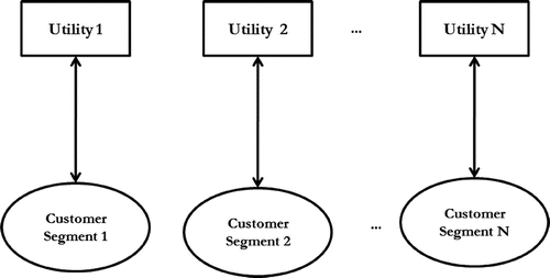
Deregulation of electricity market seeks to vertically separate potentially competitive segments e.g. generation, marketing and retail supply. Transmission and distribution systems can be run as regulated monopolies. Utilities buy varying amounts of electricity from generators at wholesale market and retails it to customers. Deregulation intends to benefit customers by allowing them to choose their preferred price and service quality combination from among several utility companies operating at the market (Joskow, 2008). Figures 1 and 2 illustrates interactions between customers and utility companies in vertically and horizontally integrated electricity markets, respectively.

Suppose there are N utility companies operating in N customer segments; total supply of electricity at particular hour is the sum of all electricity supplied by all N utilities at that particular hour(see Equation (1)). Likewise, total demand is equal to the sum of individual demand in N customer segments, as shown by Equation (2).(1) $$\begin{array}{cc}\hfill S_h& =\sum _{i=1}^N{S}_{i,h}\hfill \end{array}$$(1) (2) $$\begin{array}{cc}\hfill D_h& =\sum _{i=1}^N{D}_{i,h}\hfill \end{array}$$(2) (3) $$\begin{array}{cc}\hfill S_h& \ne D_h\hfill \end{array}$$(3)

Figure 1. Interaction between utility company and individual residences.

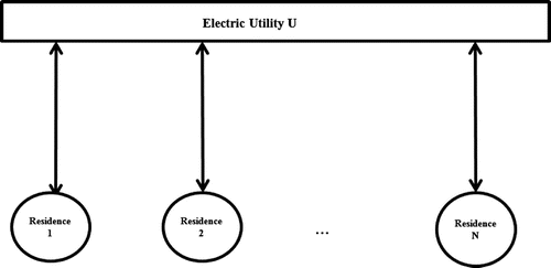
Figure 2. Interactions among utility companies and customer segments.

Having multiple utilities serving different customers in a given market presents a situation where total supply of electricity varies as well as the total demand, as in Equation (3). Moreover, utilities may have no incentive to share their supply information because of competition among them. Hence, the market can be modeled as Potluck Problem.

3.2. The Potluck problem

The Potluck problem refers to a scenario where people attend dinner regularly and each person decides how much to contribute to the dinner by considering last dinner’s supply and demand. There is no coordination among people going to the dinner. The dinner is enjoyable if both there are no leftovers and there is no starvation. Demand for food for an individual varies from time to time depending on the appetite (Enumula & Rao, 2010; Totamane, Dasgupta, & Rao, 2009). The Potluck problem is prone to oscillations where there is alternation between starvation and excess food because of rational learning. With rational learning, people will decrease their contributions for next dinner if there was excess food at last dinner and vice versa if there was starvation (Enumula & Rao, 2010; Totamane et al., 2009).

Several predictors with their associated weights and non-rational learning are used to predict demand at future dinner instances and therefore address oscillatory nature of the Potluck problem. Since several predictors are used, a Weighted Majority Algorithm (WMA) is used to determine the overall demand. Weight of correct predictors is increased at each instance while that of wrong ones is decreased. Initially, all predictors have equal (or unequal) weight (Enumula & Rao, 2010; Totamane et al., 2009). In case one prefers to assign unequal weights, more accurate predictors are assigned more weight and vice versa for less accurate ones.

Various works have used the idea of Potluck Problem to determine demand–supply equilibrium. In Maity and Rao (2010), demand and supply of solar-powered microgrids have been modeled as Potluck problem, where the residences can act as suppliers and consumers. Work by Singh and Rao (2010) models IT data centers as a Potluck problem with the intention of reducing cost of electricity with Servers as consumers and suppliers. In Totamane et al. (2009), demand and supply of air cargo is modeled as a Potluck problem with airlines as consumers and suppliers of air cargo services. In each case, non-rational learning has been used because rational learning leads to oscillation of demand and supply. Potluck problem idea has also been used in Bell, Sethares, and James (2003) and Bell and Sethares (2001). Demand–Supply equilibrium in these works is primarily single level as it is done on a daily basis, unlike deregulated electricity market where equilibrium need to be achieved on a given day and hour. Moreover, work by Maity and Rao (2010) seeks to establish a cost-neutral village by addressing per residence demand and supply. This approach may not be scalable to regional and national level to address demand and supply variability.

3.3. Application to deregulated electricity market

In a deregulated market, utilities buy electricity at wholesale price from generating companies and sell to consumers at retail price (Joskow, 2008). To model the market as Potluck problem, the utilities are assumed to be suppliers and consumers (through their customers) of electricity. This work intends to establish an optimal position where the supply of electricity at any particular hour is equal to the total demand of electricity at that hour.

In Game Theory terms, the Potluck problem can be classified as a repeated, non-cooperative game in a system where there are both multiple producers and consumers (Totamane et al., 2009). The players (agents) in the game act in order to avoid starvation or excess resource using historical data. This means no player can benefit from a unilateral move, hence securing a Social Welfare where equilibrium is attained between demand and supply (Radziszewska, Kowalczyk, & Nahorski, 2014). In deregulated electricity market, it is in the interest of ISO to ensure Social Welfare is achieved at any time slot (game instance).

Suppose there are N utility companies in a given electricity market. These are players in a game. Consider demand and supply of electricity in a given day of a single utility at hour $h\in \mathcal{H}\triangleq \{1,2,\dots ,H\}$, where $H=24$ hours. Furthermore, consider an instance t (a particular day) of a game at hour h. A player $i\le N$ has a strategy space $0\le Q_i\le {\text{Max}}_i$, where $Q_i$ is the amount of electricity supplied by player i and $Ma{x}_i$ is the maximum amount of electricity that can be supplied by player i. Considering $M_i$ as a set of probability distributions over $Q_i$ which defines mixed strategy for player i; $S_{i,h,t}\in M_i$ indicates a mixed strategy for player i at game instance t at hour h. Total amount of electricity supplied by players at hour h at t game instance is given by Equation (12). The player makes decision based on the mixed strategy $S_{i,h,t}$ by predicting the total demand of electricity $P_{i,h,t}$ (see Equation (13)) at hour h and game instance t. The utilities (players) have been considered to be both producers and consumers of electricity through customers they serve. Therefore, $d_{i,h,t}$ is used to denote demand of electricity of player i at hour h during game instance t. Total demand of electricity for all players at game instance h is as indicated in Equation (13). In this work, we seek to establish an equilibrium position where $S_h=D_h$ since if $S_{h,t}<D_{h,t}$ then there will be blackouts and $S_{h,t}>D_{h,t}$ means there is wastage of electricity. Storing excess electricity is expensive and inefficient (Vinois, 2012).(4) $$\begin{array}{cc}\hfill S_{h,t}& =\sum _i^N{S}_{i,h,t}\hfill \end{array}$$(4) (5) $$\begin{array}{cc}\hfill D_{h,t}& =\sum _i^N{d}_{i,h,t}\hfill \end{array}$$(5)

Since using rational learning in predicting demand results in oscillations; instead, non-rational learning is used where various predictors are used and those providing a correct prediction are trusted more than ones giving wrong predictions. This is natural as experts with correct advice are trusted more than those giving wrong ones. The trust is represented by a certain weight and initially all predictors may have the same weight. Total demand prediction of electricity is obtained by using a weighted average of all predictors. Predictors make use of historical data about demand and supply of electricity to predict future needs and consumption of it. With electricity, prices as well as demand and supply tend to vary from time to time. In this case, the predictor should make use of past data at a particular hour to predict future demand at that hour. That is, a predictor should be a function that makes use of $S_{h,t-1},S_{h,t-2},\dots ,S_{h,t-x}$ (past x electricity supply data at hour h) and $D_{h,t-1},D_{h,t-2},\dots ,D_{h,t-x}$ (past x electricity demand data at hour h) to predict next supply and demand of electricity ($S_{h,t}$ and $D_{h,t}$ respectively) at hour h. In this work, predictors 1–5 have been used as suggested by Maity and Rao (2010), Enumula and Rao (2010) and Totamane (2009). Additionally, a new predictor (see item 6) with values comparable to that of item 1 has been introduced.

(1)	Average Predictor (AVP): Predicts demand as the average of all demands of electricity over last x game instances(days) at hour h as shown in Equation (6): (6) $$\begin{array}{c}\hfill \text{AVP}=\frac{D_{h,t-1}+D_{h,t-2}+\cdots +D_{h,t-x}}{x}\end{array}$$(6)
(2)	Random Predictor (RNP): Randomly chooses values for demand of electricity over past x game instances at hour h. Mathematically, RNP is a random variable following the discrete uniform distribution over set $D_{h,t-1},D_{h,t-2},\dots ,D_{h,t-x}$
(3)	Rational Predictor (RTP): the demand of electricity at game instance h is the same as one on previous day. Given $D_{h,t-1},D_{h,t-2},\dots ,D_{h,t-x}$, RTP is calculated as in Equation (7): (7) $$\begin{array}{c}\hfill \text{RTP}=D_{h,t-1}\end{array}$$(7)
(4)	Maximum Predictor (MXP):Takes largest demand of electricity over last x game instances at hour h (See Equation (8)). (8) $$\begin{array}{c}\hfill \text{MXP}=max\{D_{h,t-1},D_{h,t-2},\dots ,D_{h,t-x}\}\end{array}$$(8)
(5)	Minimum Predictor (MNP): The smallest demand of electricity over last x game instances at hour h (Equation (9)). (9) $$\begin{array}{c}\hfill \text{MNP}=min\{D_{h,t-1},D_{h,t-2},\dots ,D_{h,t-x}\}\end{array}$$(9)
(6)	MinMaxAverage (NXA): the average of minimum and maximum demand of electricity over x game instances at hour h. Equation (10) indicates how the predictor is obtained: (10) $$\begin{array}{c}\hfill \text{NXA}=\frac{\text{MXP}+\text{MNP}}{2}\end{array}$$(10)

The predictors 1–6 have been used to compute predicted demand, $P_{i,h,t}$. The Potluck problem with non-rational learning is flexible enough that additional predictors can be added. For instance, a regulator may want to influence demand prediction based on some information not available to utilities by introducing a new predictor to all utilities. Likewise, a time-based predictor (Enumula & Rao, 2010) can be introduced to predict demand according to time of the day, weekdays vs. weekends as electricity consumption varies accordingly. Moreover, predictors that take into account explanatory variables such as temperature, calendar events and seasonality would add value to the quality of prediction.

Table 1. Description of symbols used

Symbol	Definition
N	Number of utilities
h	Particular hour
t	Particular day
i	Specific utility company
H	2,400 h, or 0000 h
$\mathcal{H}$	A set of 24 hours in a day
K	Maximum number of predictors
k	Number of chosen predictors
p	Specific predictor (e.g. AVP, MXP, etc)
$\mathit{\beta }$	Constant parameter between 0 and 1 that measures how drastic are changes in predictions.
$\mathit{\gamma }$	Determines to what extent a predictor should be penalized or rewarded based on its accuracy
x	Number of past data available for prediction
F	Pool of predictors
$D_{h,t}$	Demand at hour h on day t.
$D_{i,h}$	Demand at hour h, to be served by utility i
$D_h$	Total Demand at hour h,
$S_{h,t}$	Supply at hour h on day t
$S_{i,h}$	Amount of electricity supplied by utility i at hour h
$S_h$	Total Supply at hour h
$W_{i,p,h,t}$	Weight of a predictor p for utility i at hour h for day t
$O_{i,p,h,t}$	Predicted electricity demand for a specific utility i at hour h, day t
$S_{i,h,t}$	Particular utility’s amount of electricity it is supposed to Supply to customers at hour h, day t
$d_{i,h,t}$	Particular utility’s demand of electricity at hour h, day t
$P_{i,h,t}$	Aggregate Predicted Demand by utility i, at hour h on day t

Suppose there are K predictors, each of the N utility companies chooses k ($k\le K$) predictors randomly or based on some criteria such as computational efficiency and availability. Each utility company has k predictions for demand at game instance t at hour h. Each of the predictions is denoted by $O_{i,p,h,t}$ which refers to the prediction of utility i for game instance t at hour h using predictor p. $O_{i,p,h,t}$ is computed by one of AVP, RNP, RTP, MXP, MNP, or NXA. Each predictor is associated with a weight $W_{i,p,h,t}$ which is updated on every iteration of the game. In each step, the weight of accurate predictors is increased (or remains constant) while that of inaccurate ones is decreased. Initially, all predictors have the same non-zero weight. The predictors may also be initialized with some predetermined values or some random values. Using weighted majority, the utility i decides to supply $S_{i,h,t}$ based on demand predicted (i.e. $P_{i,h,t}$) by the k predictors (see Equation (3)), taking into account its market share and electricity loss in transmission and distribution lines.

After each hour h, a utility updates the weights of all its predictors depending on their performance in the previous hour, with regard to actual observed demand. It is done by multiplying the weights of predictors by F which denotes a pool of experts, as shown in Equation (12). F depends on two other parameters: $\mathit{\beta }$ and $\mathit{\gamma }$ (see Equation (13)). As noted in Totamane (2009), $\mathit{\beta }$ is a measure of how drastic predictions change over iterations. Smaller values of $\mathit{\beta }$ indicates more drastic changes, and vice versa is true. That is why in some cases, the algorithm may not converge because of too small values of $\mathit{\beta }$, as observed in this work. While $\mathit{\beta }$ is constant, $\mathit{\gamma }$ varies depending on the accuracy of predictors as in Equation (14). In Equation (15), the updated weights are normalized so that they are between 0 and 1. Symbols associated with Equations (1) to (15) are explained in Table 1.(11) $$\begin{array}{cc}& P_{i,h,t}=\frac{{\sum }_{p=1}^k(W_{i,p,h,t}\times O_{i,p,h,t})}{{\sum }_{p=1}^k{W}_{i,p,h,t}},p=1,2,\dots ,k\hfill \end{array}$$(11) (12) $$\begin{array}{cc}& W_{i,p,h,t+1}=W_{i,p,h,t}\times F\hfill \end{array}$$(12) (13) $$\begin{array}{cc}& F={\mathit{\beta }}^{\mathit{\gamma }},\text{where}0<\mathit{\beta }<1\hfill \end{array}$$(13) (14) $$\begin{array}{cc}& \mathit{\gamma }=\left\{\begin{array}{cc}\frac{O_{i,p,h,t}}{D_{h,t}}\hfill & \text{if}\frac{O_{i,p,h,t}}{D_{h,t}}>1\hfill \\ frac{D}_{h,t}{O}_{i,p,h,t},\hfill & \text{otherwise}.\hfill \end{array}\right.\hfill \end{array}$$(14) (15) $$\begin{array}{cc}& W_{i,p,h,t+1}=\frac{W_{i,p,h,t+1}}{{\sum }_{p=1}^k{W}_{i,p,h,t+1}}\hfill \end{array}$$(15)  

4. Proposed algorithm

Based on description of the Potluck Problem and non-rational learning algorithm in Section 3, Algorithm was developed. Every utility company runs the algorithm independently. It is assumed all utilities are connected to both electric grid and communication network. Past data on demand and supply are accessible to all utility companies and are the same. The algorithm can be summarized in steps as follows:

(1)	For each day and hour, each utility company selects predictors to be used.
(2)	Using past data on demand and supply, and chosen predictors, the utility predicts demand using each of the predictors.
(3)	The utility predicts aggregate demand using all predictors with WMA.
(4)	Based on predicted aggregate demand, the utility decides on total supply and on what it should supply taking into account possible transmission and distribution line losses and its market share.
(5)	Checks actual demand and supply experienced at that hour.
(6)	Updates weights of predictors based on actual demand and supplied experienced on that hour.
(7)	Update past data with actual demand and supply.

See Algorithm for more details.

5. Simulation, results and discussion

A deregulated electricity market with four (4) utility companies was simulated for twenty five (25) game instances (days). Predictors made use of 10 past consumption patterns at any given hour(i.e. $x=10$). Hourly demand and supply data for March to June 2016 from Danish electricity market were used to test and analyzed the proposed algorithm (Energinet, 2016).

Figure 3. Weight of predictors after convergence.

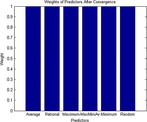
Six predictors ($K=6$) have been used in this simulation as discussed in Section All predictors had their weight initialized to 1. At each game instance, each utility randomly chose four (4) predictors ($k=4$). After convergence, all predictors ended up with similar values close 0.9 as illustrated in Figure 3. Final weights are smaller than initial ones because predictors get penalized when predicted demand is different from the actual ones.

In some cases, one may want to assign different weights to predictors, for example AVP is more representative of consumption pattern as it makes use of all past data. It is reasonable to assign more weight to it. If weights assigned previously are not the same, the final ones may also not be the same, depending on the performance of the predictors. Since the predictors were drawn at random at each hour and for each utility, their frequency of use may differ from time to time as shown in Figure 4.

Figure 4. Frequency of use of each predictor.

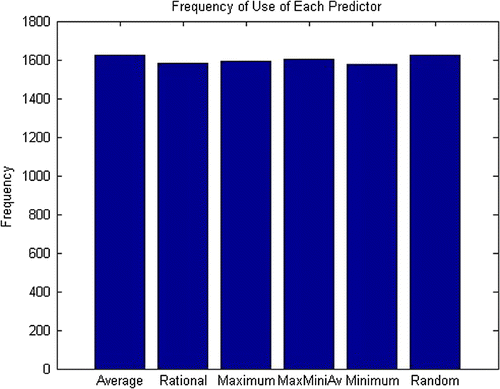
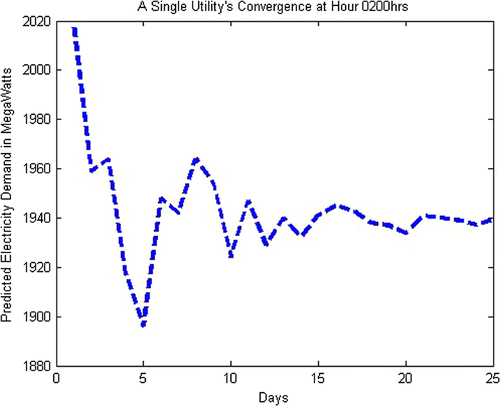
Figure 5. Convergence of a single utility at 0200 h.

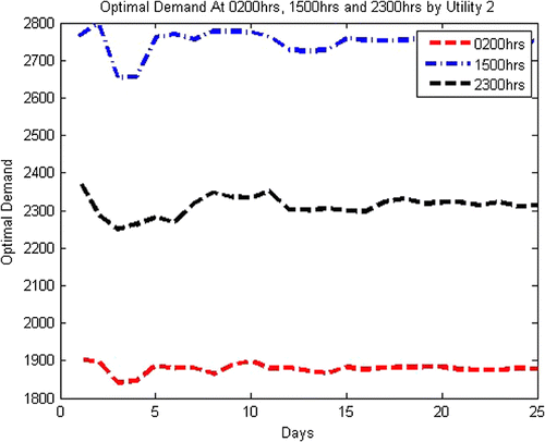
Although $\mathit{\beta }$ values in the range 0 to 1 (exclusive) have been suggested, the system converges for $0.9\le \mathit{\beta }<1$. Otherwise, the system diverges. The proposed algorithm was simulated with parameter $\mathit{\beta }=0.996$. It was observed that the resulting system started to converge on the 12th instance of the game with all utilities ending with roughly the same demand value at a particular hour as indicated in Figure 5 and 10. This is because the algorithm takes some time to learn the usage patterns, which means the algorithm can be separated into training and learning parts so that utilities converge right away.

Figure 6. Comparison between actual demand and optimal demand.

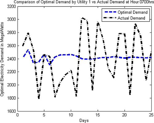
Figure 6 provides a contrast between Actual Demand and Optimal Demand. It means variability of demand and supply can be reduced using the proposed algorithm as optimal demand gets steady with each game instance. Discrepancy between actual demand and optimal demand can be as small as 0.046% and as high as 33.36% (see Tables 2–5). Figure 7 indicates Mean Absolute Percentage Error (MAPE) between Actual and Optimal Demand for all four utilities. It can be observed that MAPE ranges from 5 to 33%. Although in some cases discrepancy values and MAPE values are significant, what matters is reduction in demand variation while taking into account past consumption patterns as observed in Figure 6.

Figure 8 indicates convergence of all four utilities at 2,200 h. It can be observed that although utilities may pick different predictors, they all end up with same or similar demand. Moreover, the figure indicates that as the system learns about consumption behavior, predictions get steady.

Figure 7. Daily mean absolute percentage error for all four utilities.

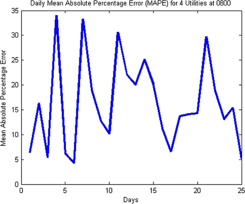
Figure 8. Convergence of four utilities at 2,200 h.

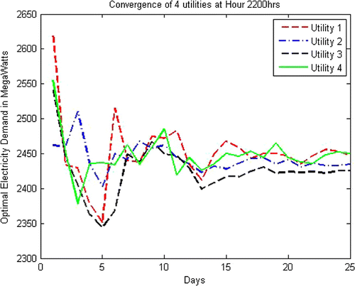
Figure 9. Demand-supply variability with Consumers as Potluck problem agents.

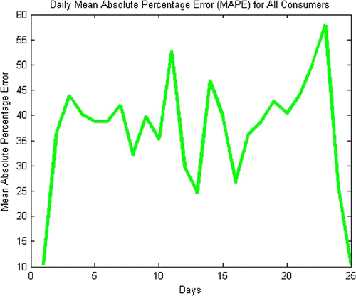
Figure 10. Convergence at different hours for a single utility.

Several works have employed non-cooperative games to model electricity markets (Atzeni, Ordóñez, Scutari, Palomar, & Fonollosa, 2013; Hazem, 2014; Jalali & Kazemi, 2015; Maity & Rao, 2010). With the exception of Jalali and Kazemi (2015) and Maity and Rao (2010), most works have assumed single utility company and therefore focuses on the demand-side of the market. In Jalali and Kazemi (2015), multiple utility companies have been taken into account in the supply-side, plus interaction of customers in the demand-side. It is assumed utilities are seeking to make profit and therefore the problem addressed in the supply-side is profit maximization through a bidding mechanism. While utilities may be interested in maximizing profits, the ISO may need to ensure demand and supply matches at all times so as to enhance grid stability and reliability as presented in this work.

Table 2. Actual demand vs. optimal demand for utility 1

Hour	Actual	Optimal	% Discrepancy
0100	1,911.8	1,934	1.16
0200	1,753.5	1,939	10.58
0300	1,764.4	1,854	5.08
0400	1,874.2	1,873	0.06
0500	1,902.5	1,925	1.18
0600	2,116.1	2,060	2.65
0700	2,514.8	2,419	3.81
0800	2,154	2,720	26.28
0900	2,117.5	2,812	32.80
1000	2,915.7	2,858	1.98
1100	2,968.1	2,878	3.04
1200	2,778.4	2,956	6.39
1300	2,182.4	2,759	26.42
1400	2,123.9	2,822	32.87
1500	2,229.6	2,744	23.07
1600	2,120.7	2,690	26.84
1700	2,434.7	2,675	9.87
1800	2,674.7	2,903	8.54
1900	2,751.5	2,946	7.07
2000	2,510.7	2,748	9.45
2100	2,347.7	2,572	9.55
2200	2,053.8	2,459	19.73
2300	1,983.2	2,276	14.76
2400	1,994	2,126	6.62

Table 3. Actual demand vs optimal demand for utility 2

Hour	Actual	Optimal	% Discrepancy
0100	1,911.8	1,970	3.04
0200	1,753.5	1,878	7.10
0300	1,764.4	1,890	7.12
0400	1,874.2	1,863	0.60
0500	1,902.5	1,901	0.08
0600	2,116.1	2,013	4.87
0700	2,514.8	2,397	4.68
0800	2,154	2,707	25.67
0900	2,117.5	2,824	33.36
1000	2,915.7	2,834	2.80
1100	2,968.1	2,930	1.28
1200	2,778.4	2,882	3.73
1300	2,182.4	2,750	26.01
1400	2,123.9	2,732	28.63
1500	2,229.6	2,752	23.43
1600	2,120.7	2,644	24.68
1700	2,434.7	2,712	11.39
1800	2,674.7	2,904	8.57
1900	2,751.5	2,932	6.56
2000	2,510.7	2,841	13.16
2100	2,347.7	2,641	12.49
2200	2,053.8	2,452	19.39
2300	1,983.2	2,314	16.68
2400	1,994	2,102	5.42

Table 4. Actual demand vs. optimal demand for utility 3

Hour	Actual	Optimal	% Discrepancy
0100	1,911.8	1,953	2.16
0200	1,753.5	1,908	8.81
0300	1,764.4	1,848	4.74
0400	1,874.2	1,876	0.10
0500	1,902.5	1,899	0.18
0600	2,116.1	1,969	6.95
0700	2,514.8	2,392	4.88
0800	2,154	2,644	22.75
0900	2,117.5	2,796	32.04
1000	2,915.7	2,929	0.46
1100	2,968.1	2,931	1.25
1200	2,778.4	2,839	2.18
1300	2,182.4	2,755	26.24
1400	2,123.9	2,770	30.42
1500	2,229.6	2,773	24.37
1600	2,120.7	2,635	24.25
1700	2,434.7	2,696	10.73
1800	2,674.7	2,898	8.35
1900	2,751.5	2,936	6.71
2000	2,510.7	2,787	11.00
2100	2,347.7	2,610	11.17
2200	2,053.8	2,437	18.66
2300	1,983.2	2,273	14.61
2400	1,994	2,091	4.86

Table 5. Actual demand vs. optimal demand for utility 4

Hour	Actual	Optimal	% Discrepancy
0100	1,911.8	1,947	1.84
0200	1,753.5	1,876	6.99
0300	1,764.4	1,876	6.33
0400	1,874.2	1,889	0.79
0500	1,902.5	1,892	0.55
0600	2,116.1	2,054	2.93
0700	2,514.8	2,329	7.39
0800	2,154	2,661	23.54
0900	2,117.5	2,762	30.44
1000	2,915.7	2,764	5.20
1100	2,968.1	2,917	1.72
1200	2,778.4	2,844	2.36
1300	2,182.4	2,780	27.38
1400	2,123.9	2,681	26.23
1500	2,229.6	2,683	20.34
1600	2,120.7	2,658	25.34
1700	2,434.7	2,665	9.46
1800	2,674.7	2,866	7.15
1900	2,751.5	2,904	5.54
2000	2,510.7	2,748	9.45
2100	2,347.7	2,654	13.05
2200	2,053.8	2,455	19.53
2300	1,983.2	2,327	17.34
2400	1,994	2,102	5.42

Work by Maity and Rao (2010) considers the potential of microgrids in island mode to share excess electricity produced with nearby one. Potluck problem with non-rational learning is used to balance supply and demand with customers acting as both producers and consumers of electricity. Based on residential consumption data from OpenEI (2017), each consumer’s optimal demand for every hour was established using demand profiles of 100,000 consumers. Figure 9 illustrates that MAPE for aggregate optimal demand of consumers versus aggregate actual demand varies between 10.4 and 57.9%. Compared with MAPE values obtained in this work (5–33%), it can be argued modeling utilities as potluck agents rather than consumers is more effective in reducing variability between demand and supply. Moreover, modeling consumers as potluck agents is likely to increase cost of smart meters due to additional processing and memory requirements.

Demand and supply parity on the grid is important so as to avoid wastage of electricity in case there is excess supply and blackouts when there is shortage of it. The proposed algorithm can be used to reduce supply–demand variability without requiring active participation of the customers. Moreover, it is cost effective as it can make use of existing communication infrastructure for sharing historical consumption data.

6. Conclusion

Deregulation of electricity markets presents an opportunity for competition among utility companies with a potential for better prices and services to customers. However, it also means that variability of both demand and supply is introduced. In this work, the Potluck problem with non-rational learning has been used to address demand–supply variability problem by predicting optimal demand of electricity at each hour. Active participation of customers to attain the equilibrium (as it is the case in some works) is not necessary. Since in a deregulated market utilities have customer segments (regions, zones) and don’t operate on an entire market; scheduling algorithms can be used with the proposed algorithm for demand side management by encouraging uses to spend more electricity during off-peak hours and reduce consumption at peak hours, resulting in cost savings for both utilities and customers.

Additional information

Funding

This work was supported by Nelson Mandela African Institution of Science and Technology.

Notes on contributors

Daniel Ngondya

Daniel Ngondya earned a bachelor’s degree in 2005 and a master’s degree in 2012 from the University of Dar es Salaam. Presently, he is pursuing a doctoral degree in Information and Communication Science and Engineering at Nelson Mandela African Institution of Science and Technology (NM-AIST). He has interests in Broadband Power Line Communications and SmartGrids. This work is part of ongoing research to investigate efficient interactions between utilities and consumers in deregulated electricity market in order to manage demand.

Joseph Mwangoka

Joseph Mwangoka , PhD, is a Senior Lecturer at Nelson Mandela African Institution of Science and Technology (NM-AIST), with interests in Software Engineering, Computer Communications and Artificial Intelligence.

Appendix 1

Tables 2–4 indicating percentage discrepancy of optimal demand vs. Actual Demand for each of the four utilities; and Figure 10 illustrating convergence of demand at different hours.

References

- Atzeni, I., Ordóñez, L. G., Scutari, G., Palomar, D. P., & Fonollosa, J. R. (2013). Noncooperative and cooperative optimization of distributed energy generation and storage in the demand-side of the smart grid. IEEE Transactions on Signal Processing, 61(10), 2454–2472.
- Bell, A. M., & Sethares, W. A. (2001). Avoiding global congestion using decentralized adaptive agents. IEEE Transactions on Signal Processing, 49(11), 2873–2879.
- Bell, A. M., Sethares, W., & James, B. (2003). Coordination failure as a source of congestion in information networks. IEEE Transactions on Signal Processing, 51(3), 875–885.
- Bose, S., Wu, C., Xu, Y., Wierman, A., & Mohsenian-Rad, H. (2014). A unifying market power measure for deregulated transmission-constrained electricity markets. IEEE Transactions on Power Systems, 30(5), 2338–2348.
- Bu, H., & Nygard, K. (2014). Adaptive scheduling of smart home appliances using fuzzy goal programming. In The Sixth International Conference on Adaptive and Self-Adaptive Systems and Applications, ADAPTIVE (pp. 129–135). Citeseer.
- Cardenas, A. A., Roosta, T., & Sastry, S. (2009). Rethinking security properties, threat models, and the design space in sensor networks: A case study in scada systems. Ad Hoc Networks, 7(8), 1434–1447.
- Dai, Y., & Gao, Y. (2014). Real-time pricing decision making for retailer-wholesaler in smart grid based on game theory. In Abstract and Applied Analysis (Vol. 2014). Hindawi Publishing Corporation.
- Doorman, G. (2003). Capacity subscription and security of supply in deregulated electricity markets. SINTEF Energy Research.
- Ela, E., Milligan, M., & Kirby, B. (2011). Operating reserves and variable generation. Contract, 303, 275–3000.
- Energinet. (2016). Download of market data-production and consumption. Retrieved October 15, 2016, from http://energinet.dk/EN/El/Engrosmarked/Udtraek-af-markedsdata/Sider/default.aspx
- Enumula, P. K., & Rao, S. (2010). The potluck problem. Economics Letters, 107(1), 10–12.
- Fadlullah, Z. M., Quan, D. M., Kato, N., & Stojmenovic, I. (2014). Gtes: An optimized game-theoretic demand-side management scheme for smart grid. Systems Journal, IEEE, 8(2), 588–597.
- Faruqui, A., & Eakin, K. (2012). Pricing in competitive electricity markets (Vol. 36). New York, NY: Springer Science & Business Media.
- Griffin, J. M., & Puller, S. L. (2009). Electricity deregulation: Choices and challenges (Vol. 4). Chicago, IL: University of Chicago Press.
- Holtschneider, T., & Erlich, I. (2012). Modeling demand response of consumers to incentives using fuzzy systems. In Power and Energy Society General Meeting, 2012, IEEE (pp. 1–8). IEEE.
- Ilic, M., Galiana, F., & Fink, L. (2013). Power systems restructuring: Engineering and economics. Springer Science & Business Media.
- Jalali, M. M., & Kazemi, A. (2015). Demand side management in a smart grid with multiple electricity suppliers. Energy, 81, 766–776.
- Joskow, P. L. (2008). Lessons learned from electricity market liberalization. The Energy Journal, 29(2), 9–42.
- Joung, M. (2008). Game-theoretic equilibrium analysis applications to deregulated electricity markets. ProQuest.
- Khan, M. A., Javaid, N., Mahmood, A., Khan, Z. A., Alrajeh, N. (2015). A generic demandside management model for smart grid. International Journal of Energy Research, 39(7), 954–964.
- Kirschen, D. S. (2003). Demand-side view of electricity markets. IEEE Transactions on Power Systems, 18(2), 520–527.
- Kishore, S., & Snyder, L. V. (2010). Control mechanisms for residential electricity demand in smartgrids. In Smart Grid Communications (SmartGridComm), 2010 First IEEE International Conference on (pp. 443–448). IEEE.
- Kleit, A. N. (2007). Electric choices: Deregulation and the future of electric power. Rowman & Littlefield.
- Kumar, A., & Sekhar, C. (2012). Dsm based congestion management in pool electricity markets with facts devices. Energy Procedia, 14, 94–100.
- Lewis, N. S., & Nocera, D. G. (2006). Powering the planet: Chemical challenges in solar energy utilization. Proceedings of the National Academy of Sciences, 103(43), 15729–15735.
- Maity, I., & Rao, S. (2010). Simulation and pricing mechanism analysis of a solar-powered electrical microgrid. Systems Journal, IEEE, 4(3), 275–284.
- Matallanas, E., Castillo-Cagiga, M., Gutirrez, A., Monasterio-Huelin, F., Caamao-Martn, E., Masa, D., & Jimnez-Leube, J. (2012). Neural network controller for active demand-side management with pv energy in the residential sector. Applied Energy, 91(1), 90–97.
- Mohsenian-Rad, A.-H., & Leon-Garcia, A. (2010). Optimal residential load control with price prediction in real-time electricity pricing environments. Smart Grid, IEEE Transactions on, 1(2), 120–133.
- Momoh, J. (2012). Smart grid: Fundamentals of design and analysis (Vol. 63). John Wiley & Sons.
- Müsgens, F., Ockenfels, A., & Peek, M. (2014). Economics and design of balancing power markets in germany. International Journal of Electrical Power & Energy Systems, 55, 392–401.
- US Department of Energy. (2015). An assessment of energy technologies and research opportunities (Technical report). Author.
- OpenEI. (2017). Residential load data. Retrieved August 3, 2017, from http://en.openei.org/datasets/files/961/pub/RESIDENTIAL_LOAD_DATA_E_PLUS_OUTPUT/BASE/
- Oulton, N. (2007). Ex post versus ex ante measures of the user cost of capital. Review of Income and Wealth, 53(2), 295–317.
- Palensky, P., & Dietrich, D. (2011). Demand side management: Demand response, intelligent energy systems, and smart loads. IEEE Transactions on Industrial Informatics, 7(3), 381–388.
- Radziszewska, W., Kowalczyk, R., & Nahorski, Z. (2014). El farol bar problem, potluck problem and electric energy balancing-on the importance of communication. In Computer Science and Information Systems (FedCSIS), 2014 Federated Conference on. IEEE. (pp. 1515–1523)
- Rassenti, S. J., Smith, V. L., & Wilson, B. J. (2002). Demand-side bidding will reduce the level and volatility of electricity prices. INDEPENDENT REVIEW-OAKLAND, 6(3), 441–446.
- Ruelens, F., Claessens, B., Vandael, S., Schutter, B. D., Babuska, R., & Belmans, R. (2015). Residential demand response applications using batch reinforcement learning. arXiv preprint arXiv:1504.02125.
- Singh, N., & Rao, S. (2010). Modeling and reducing power consumption in large it systems. In Systems Conference, 2010 4th Annual IEEE (pp. 178–183). IEEE.
- Soliman, H. M., & Leon-Garcia, A. (2014). Game-theoretic demand-side management with storage devices for the future smart grid. IEEE Transactions on Smart Grid, 5(3), 1475–1485.
- Totamane, R., Dasgupta, A., & Rao, S. (2009). Air cargo demand modeling and prediction. Systems Journal, IEEE, 8(1), 52–62.
- Ulbig, A., Borsche, T. S., & Andersson, G. (2014). Impact of low rotational inertia on power system stability and operation. IFAC Proceedings Volumes, 47(3), 7290–7297.
- Vinois, J. (2012). Dg ener working paper: The future role and challenges of energy storage. European Commission, Director-General for Energy.
- Walawalkar, R. S. (2008). Economics of emerging electric energy storage technologies and demand response in deregulated electricity markets. ProQuest.
Appendix 1
Tables – indicating percentage discrepancy of optimal demand vs. Actual Demand for each of the four utilities; and Figure illustrating convergence of demand at different hours.