Robust optimal control for a class of nonlinear systems with uncertainties and external disturbances based on SDRE

Abstract

In this paper, the problem of the robust optimal control (ROC) for a class of nonlinear systems with uncertainties and external disturbances is studied. For this purpose, the State Dependent Riccati Equation (SDRE) is considered as a solution of the ROC. The proposed method is to transform a robust control problem into an optimal control problem, where the uncertainties and disturbances are reflected in the performance index. Hence, the performance index is selected as an energy function and using the proposed constraints in this paper the Lyapunov stability for this class of nonlinear systems is proved and the robust optimal controller is designed. In order to illustrate the high capability of the ROC method in optimal control of complex systems such as Hyper-chaotic system, the time response of state variables in the proposed method and the Global Robust Optimal Sliding Mode Control (GROSMC) method are compared together. The simulation results show that the time response of state variables in the ROC method is more sufficient than the GROSMC method.

Keywords:

• nonlinear system
• optimal control
• robust optimal control
• sliding mode control
• uncertainty
• external disturbance
• Lyapunov stability
• SDRE

View correction statement:

Corrigendum

Public Interest Statement

In this paper, the problem of optimal control for a class of affine nonlinear systems with uncertainties and external disturbances is studied. For this purpose, the SDRE method was considered as an optimal solution and then by replacing a few simple constraints and extending the SDRE controller, the ROC controller was obtained. In order to expand the robust optimal controller (ROC) in future work, it is proposed to extend this method to a wider class of nonlinear systems, such as $\dot{x}=f(x)+g(x,u)$ or $\dot{x}=f(x,u)$. Also, in order to enhance the time response capability, the intelligent methods can be used to optimize the weight parameters in the SDRE and the ROC methods.

1. Introduction

By examining nonlinear systems, it can be realized that there is no single optimal control law for controlling those systems, and usually the scientists attempt to find a solution of near optimum, which can be acceptable. Thus, According to the conditions of the problem, a solution should be selected that has the closest response to the optimal value. The purpose of optimal control is to determine the control laws, which satisfy the physical constraints and at the same time minimize or maximize the certain performance index. The performance index can be defined based on the requirements from the effective physical factors and the expectation from a system.

In nonlinear systems, various approximate techniques can be applied to obtain optimal control law. Since, there is no definite formula for the optimal solution of nonlinear systems, different semi-optimal methods are suggested for those systems (Burghart, 1969; Garrard, McClamroch, & Clark, 1967; Pearson, 1962; Wernli & Cook, 1975). One of the most effective methods is to solve the optimal feedback control for the nonlinear systems by solving a SDRE equation (Beeler, Tran, & Banks, 2000a, 2000b; Krikelis & Kiriakidis, 1992; Wang, Yaz, & Long, 2014). An optimal feedback control is studied by Krikelis and Kiriakidis that satisfied the Hamiltonian-Jacobin–Bellman (HJB) equations (Krikelis & Kiriakidis, 1992). Beeler et al. investigated a comparison of several methods for the synthesis of nonlinear control systems (Beeler et al., 2000a, 2000b). Also, Wang et al. explored a resilient state-dependent control for continuous-time nonlinear systems with general performance index (Wang et al., 2014). Since the co-state equation is state-dependent and it develops backward and the state is not accessible in whole time, then the control law cannot be calculated. To overcome this problem, Khaloozadeh and Abdolahi proposed an iterative procedure for solving the SDRE equation (Khaloozadeh & Abdolahi, 2004).

The SDRE method has been employed by different researchers to study different nonlinear systems (Abagnale, Aggogeri, Borboni, Strano, & Terzo, 2017; Gao, Gao, Mu, & Gao, 2016; Gao, Wang, & Cheng, 2017; Nemra & Aouf, 2010; Strano & Terzo, 2016; Strano & Terzo, 2017). The SDRE could be used for state estimation in nonlinear systems (Abagnale et al., 2017; Strano & Terzo, 2016). Strano and Terzo are proposed an alternative nonlinear estimation method based on the SDRE method (Strano & Terzo, 2016). Abagnale et al. investigated the SDRE estimator that is able to fully take into account dead-zone hard nonlinearity and measurement noise (Abagnale et al., 2017). The SDRE method also as an effective method for designing nonlinear filters has been demonstrated (Gao et al., 2017; Nemra & Aouf, 2010). Nemra and Aouf presented a new INS/GPS sensor fusion scheme, based on SDRE nonlinear filtering for unmanned aerial vehicle (UAV) localization problem that SDRE navigation filter is proposed as an alternative to the extended Kalman filter (EKF) (Nemra & Aouf, 2010). In order to overcome the nonlinear nature of the vehicle, Strano and Terzo explored an alternative nonlinear estimation method based SDRE. The mentioned technique is able to fully take into account the system’s nonlinearities and the measurement noise (Strano & Terzo, 2017). Gao et al. investigated a robust adaptive filter based on SDRE method for strap-down inertial navigation system. They adopted the state dependent coefficient (SDC) to convert nonlinear system model into linear system for avoiding the errors caused by the traditional numerical linearization process. It also adopted the concepts of robust estimation and adaptive factor to construct the discriminant statistics and adaptive factor reasonably for resisting the disturbances of singular observations and kinematic model error (Gao et al., 2016, 2017). The SDRE method can be used to control a wide range of systems (Acarman, 2009; Choi, 2012; Kumar, Jerome, & Raaja, 2014; Liccardo, Strano, & Terzo, 2013; Parrish & Ridgely, 1997; Pukdeboon & Zinober, 2009a; Strano & Terzo, 2015), such as vehicle control (Acarman, 2009), hydraulic actuation (Liccardo et al., 2013; Strano & Terzo, 2015), spacecraft (Pukdeboon & Zinober, 2009a), satellite (Parrish & Ridgely, 1997), ball and beam (Kumar et al., 2014), chaotic system (Choi, 2012) and etc.

As mentioned, robust optimal controllers have been developed based on the SDRE approach. In many studies, there are a number of challenges such as uncertainty that have been examined in the parameters of nonlinear systems (Pang & Wang, 2009; Pukdeboon, 2015; Pukdeboon & Zinober, 2009b; Salamci & Gökbilen, 2007). In this regard, various techniques for designing robust optimal controllers are presented using nonlinear control methods such as sliding mode control (SMC). Salami and Goblin designed the sliding surface based on SDRE methodology for missile autopilot (Salamci & Gökbilen, 2007). Pukdeboon and Zinober investigated the two optimized SMC (OSMC) laws by using the integral sliding mode control for attitude tracking of spacecraft (ISM) (Pukdeboon, 2015; Pukdeboon & Zinober, 2009b). Pang and Wang studied a design method of the GROSMC for a class of affine nonlinear systems with uncertainties. They integrated the sliding mode control (SMC) theory with SDRE in their investigation (Pang & Wang, 2009).

In this paper, the purpose is to design an optimal control law for a class of nonlinear systems so that it is robust against uncertainties and external disturbances, also minimizes the certain performance index. This paper extends the optimal control method for robust problems and provides a Robust Optimal Control (ROC).

This paper is organized as follows:

Section 1 presents the introduction.

Section 2 presents the general view of SDRE method.

Section 3 presents the general view of GROSMC method.

Section 4 presents the ROC method via a sub-optimal control approach in the two modes.

Section 5 presents simulations of the ROC method and compares with the GROSMC method.

Section 6 presents the conclusions.

2. A general view of SDRE

The considered a class of affine nonlinear system as following forms:(1) $$\left\{\begin{array}{c}\dot{x}=f(x)+g(x)u(t)\hfill \\ x(0)=x_0\hfill \end{array}\right.$$(1)

with x ∊ R ^m , u:R ^m  → R ^k .

In SDRE method, the purpose is design an optimal control law which minimizes the following performance index:(2) $$J=\frac{1}{2}\underset{0}{\overset{\infty }{\int }}(x{(t)}^{T}Qx(t)+u{(t)}^{T}Ru(t))\text{d}t.$$(2)

The weighting matrices Q and R are semi-positive definite and positive definite, respectively. The SDRE control law by defining the Hamiltonian function Equation (3) and applying the conditions of the problem is obtained.(3) $$\text{H}(x,u)=\frac{1}{2}{x}^{T}Qx+\frac{1}{2}{u}^{T}Ru+{\lambda }^T(f(x)+g(x)u).$$(3)

The requirements are described as follows:(4) $$\dot{x}=\frac{\partial H}{\partial \lambda }=f(x)+g(x)u.$$(4) (5) $$\dot{\lambda }=-\frac{\partial H}{\partial x}=-Qx-\frac{\partial f{(x)}^T}{\partial x}\lambda -\frac{\partial g{(x)}^T}{\partial x}u\lambda .$$(5) (6) $$\frac{\partial H}{\partial u}=Ru+g{(x)}^T\lambda =0.$$(6)

The following equation is obtained by simplifying Equation (6):(7) $$u(t)=-R^{-1}g{(x)}^T\lambda (t).$$(7)

Also, λ is obtained from Equation (8):(8) $$\lambda =P(x)x.$$(8)

For this class of nonlinear systems that the state nonlinearities are linearly related to the input system matrix, it can be shown these relations as semi-linear and as follows:(9) $$\left\{\begin{array}{c}f(x)=A(x)x\hfill \\ g(x)=B(x).\hfill \end{array}\right.$$(9)

The Equation (7) can be rewritten as follows with respect to the change of λ(t) as Equation (8):(10) $$u(t)=-R^{-1}B{(x)}^{T}P(x)x.$$(10)

Considering the boundary condition p(T) = 0 and by solving the above equations, the SDRE equation is obtained as follows:(11) $$\dot{P}(x)+A{(x)}^{T}P(x)+P(x)A(x)-P(x)B(x)R^{-1}B{(x)}^{T}P(x)+Q=0.$$(11)

The SDRE can also be defined as follows:(12) $$\dot{P}(x)+(A{(x)}^T+\alpha I)P(x)+P(x)(A(x)+\alpha I)-P(x)B(x)R^{-1}B{(x)}^{T}P(x)+Q=0.$$(12)

where α is scalar design parameter which indirectly reduces the error rate in controlling makes visible the proposed (Beikzadeh & Taghirad, 2011, 2012).

Indeed, Equation (11) or (12) must be solved and by obtaining P(x) and then, the optimal control law u(t) is obtained.

3. A general view of GROSMC

Consider an uncertain affine nonlinear system described by (Pang & Wang, 2009):(13) $$\begin{array}{c}\dot{x}(t)=A(x)x+B(x)u+\delta (x,t)\hfill \\ x(0)=x_0.\hfill \end{array}$$(13)

where x(t) ∊ R ⁿ is the state vector, u(t) ∊ R ^m is the control law, A(x) ∊ C ^k , $\delta (x,t)=B\overline{\delta }(x,t)$ is the lumped uncertainty and B(x) ∊ C ^k with k ≥ 1are nonlinear function of x, respectively.

Assumption 3.1

The pair of $\{A(x),B(x)\}$ is controllable or it is at least stabilizable.

Assumption 3.2.

There are unknown positive constants γ ₀and γ ₁ so that it is satisfy in the matching conditions Equation (14).

(14) $$\left\{\begin{array}{c}\delta (x,t)=B\overline{\delta }(x,t)\hfill \\ ∥\overline{\delta }(x,t)∥\le {\gamma }_0+{\gamma }_1∥x(t)∥.\hfill \end{array}\right.$$(14)

Here $\Vert ·\Vert$ denotes the Euclidean norm.

Assumption 3.3.

The matrix G(x)B(x) is nonsingular.

Considering the above assumptions and by choosing an integral sliding surface Equation (15), robust optimal law in the GROSMC method is obtained as follows Equation (16):(15) $$\left\{\begin{array}{c}S(t,x(t))=G(x)[x(t)-x(0)]\hfill \\ -G(x){\int }_0^t[A(x)-B(x)R^{-1}{B}^T(x)P(x)]x(\tau )d\tau \hfill \\ S(0,x(0))=0.\hfill \end{array}\right.$$(15) (16) $$u=-{[G(x)B(x)]}^{-1}[G(x)\delta (x,t)+G(x)B(x)R^{-1}{B}^T(x)P(x)]$$(16)

and $G(x)\in R^{m\times n}$

It is proved that the sliding mode dynamics of uncertain system Equation (13) and optimal dynamics of the nominal system Equation (1) have the same equation. As a result, they will have the same dynamic responses.

4. The ROC method via a sub-optimal control approach

In this section, the nonlinear system is presented with uncertainties and disturbances in two modes. Then, the Lyapunov stability is discussed. Consider uncertainties and disturbances in the nonlinear system described by Equations (17) and (18):(17) $$\left\{\begin{array}{c}\dot{x}=A(x)+B(x,\theta )u(t)+B(x)w(x,t)\hfill \\ B(x,\theta )=B(x)D(\theta )\begin{array}{c}\end{array}\text{and}\begin{array}{c}\end{array}D(\theta )=I+b(\theta ).\hfill \end{array}\right.$$(17) (18) $$\left\{\begin{array}{c}\dot{x}=A(x,\theta )+B(x)u(t)+B(x)w(x,t)\hfill \\ A(x,\theta )=(A(x)+\alpha (\theta ))x.\hfill \end{array}\right.$$(18)

In the above equations, α(θ) and D(θ) display the uncertainties in the state matrix and input matrix respectively and w(x,t) represents external disturbances entered into the system. Also the constant matrix R exists such that $0\prec R\le D(\theta )$ for all θ.

In the Equation (17), uncertainties and external disturbances are in the input matrix (the state matrix does not have uncertainties) and in the Equation (18), the uncertainties are in the state matrix (the input matrix does not have uncertainties). Using the optimal control and applying the conditions that obtained during the process of proving the Lyapunov stability, the ROC problem for this class of nonlinear system is solved.

4.1. Uncertainties in the input matrix despite external disturbances

In this section, the purpose is to find an optimal control law $u(t)=u_o(t)$, so that the closed loop system Equation (17) is robust against uncertainties and external disturbances. And also minimize the following performance index (Beikzadeh & Taghirad, 2011):(19) $$\left\{\begin{array}{c}J=\frac{1}{2}\underset{0}{\overset{\infty }{\int }}(x^{T}Qx+u{(t)}^{T}Ru(t)+w^{T}w)dt\hfill \\ Q\ge 0\begin{array}{cc}\begin{array}{cc}& \text{and}\end{array}& \end{array}0\prec R\le D(\theta ).\hfill \end{array}\right.$$(19)

The SDRE equation for the ROC method becomes as follows:(20) $$\begin{array}{c}\dot{P}(x)+{(A(x)+\alpha I)}^{T}P(x)+P(x)(A(x)+\alpha I)\hfill \\ -P(x)B(x)R^{-1}D(\theta )D{(\theta )}^{T}B{(x)}^{T}P(x)+Q=0\hfill \end{array}$$(20)

where α is scalar design parameter. Also, the ROC law is obtained as follows:(21) $$u(t)=-R^{-1}{(B(x)D(\theta ))}^{T}P(x)x.$$(21)

Theorem 4.1.1

Consider the Equation (17) where b(θ) denotes uncertainty and w(x,t) is external disturbance. Using the following assumptions, the ROC law is converted to optimal control law.

Assumption 4.1.1

The pair of {A(x), B(x,θ)} is pointwise stabilizable.

Assumption 4.1.2

In order to satisfy the necessary condition of the Lyapunov stability, it’s assumed that A(0) = 0 and w(0,t) = 0.

Assumption 4.1.3.

There is a non-negative constant w, so that the external disturbances w(x,t) are limited.

(22) $$∥w(x,t)∥\le w$$(22)

In fact, the constant w is the upper bound for external disturbance to the system.

Assumption 4.1.4

The uncertainty b(θ) is a non-negative and bounded matrix.

(23) $$\left\{\begin{array}{c}\theta =\gamma (x)\hfill \\ 0\le b(\theta )\le M.\hfill \end{array}\right.$$(23)

Proof

If a solution exists for optimal control problem, then it is a solution to the robust problem. Hence, consider $u(t)=u_o(t)$ as the response to the optimal control problem. It is shown that for all uncertainties b(θ) and disturbances w(x,t), the system is asymptotically stable. For this purpose, performance index is defined as follows (Lin, 2007):

(24) $$v(x)=min\underset{0}{\overset{\infty }{\int }}(x^{T}x+u{(t)}^{T}u(t)+w^{T}w)\text{d}t.$$(24)

In fact, Equation (24) is considered as the Lyapunov function for the uncertainties system Equation (17). By definition, at least the control function v(x) must be satisfied in the HJB equation. As a result, the following relation is obtained:(25) $$\left\{\begin{array}{c}min(x^{T}x+u{(t)}^{T}u(t)+w^{T}w+v_x^T(A(x)+B(x)u(t)))=0\hfill \\ v_x=\frac{\partial v}{\partial x},u\in R^m.\hfill \end{array}\right.$$(25)

Since $u(t)=u_o(t)$ is the optimal control law, it should satisfy in Equations (21) and (25):(26) $$2u_o{(t)}^T+v_x^{T}B(x)=0.$$(26) (27) $$x^{T}x+u_o{(t)}^T{u}_o(t)+w^{T}w+v_x^T(A(x)+B(x)u_o(t))=0.$$(27)

It is shown that v(x) is the Lyapunov function for nonlinear system Equation (17).

The characteristics of a Lyapunov function are as follows:(28) $$\text{Lyapunov function}v(x)=\left\{\begin{array}{c}v(x)\succ 0\begin{array}{cc}& \end{array}if\begin{array}{c}\end{array}x\ne 0\hfill \\ v(x)=0\begin{array}{cc}& \end{array}if\begin{array}{c}\end{array}x=0.\hfill \end{array}\right.$$(28)

The following relations are employed to prove that $\dot{v}(x)\prec 0$ for x ≠ 0:(29) $$\dot{v}(x)=v_x^T\dot{x}=v_x^T(A(x)+B(x)(u_o(t)+b(\theta )u_o(t))+B(x)w(x,t)).$$(29)

By a little manipulation the above equation, we have:(30) $$\dot{v}(x)=v_x^T(A(x)+B(x)u_o(t))+v_x^{T}B(x)w(x,t)+v_x^{T}B(x)b(\theta )u_o(t).$$(30)

By replacing Equations (26) and (27) into Equation (30), one could have:(31) $$\begin{array}{c}\dot{v}(x)=-w^{T}w-x^{T}x-u_o{(t)}^T{u}_o(t)-2u_o{(t)}^{T}w(x,t)\hfill \\ -2u_o{(t)}^{T}b(\theta )u_o(t).\hfill \end{array}$$(31)

Considering that uncertainty b(θ) is positive matrix, the following relation is obtained:(32) $$\dot{v}(x)\le -w^{T}w-x^{T}x-u_o{(t)}^T{u}_o(t)-2u_o{(t)}^{T}w(x,t).$$(32)

By adding and decreasing the expression $w{(x,t)}^{T}w(x,t)$ to Equation (32) and with simplification, the following relationship is achieved:(33) $$\begin{array}{c}\dot{v}(x)\le -w^{T}w+w{(x,t)}^{T}w(x,t)-x^{T}x\hfill \\ -u_o{(t)}^T{u}_o(t)-2u_o{(t)}^{T}w(x,t)-w{(x,t)}^{T}w(x,t).\hfill \end{array}$$(33)

By simplification the above equation, we have:(34) $$\begin{array}{c}\dot{v}(x)\le -w^{T}w+w{(x,t)}^{T}w(x,t)-x^{T}x\hfill \\ -{(u_o(t)+w(x,t))}^T(u_o(t)+w(x,t)).\hfill \end{array}$$(34)

Hence, the following relation is obtained:(35) $$\dot{v}(x)\le -w^{T}w+w{(x,t)}^{T}w(x,t)-x^{T}x.$$(35)

Considering that the disturbances w(x,t) are bounded, one could have:(36) $$w{(x,t)}^{T}w(x,t)\le w^{T}w\to \dot{v}(x)\le 0.$$(36)

In other words, the system described in Equation (17) is asymptotically stable for all uncertainties and disturbances. As a result, the ROC law Equation (21) is the response of the SDRE problem. □

4.2. Uncertainties into the state matrix of system in the presence of the external disturbances

In this section, the purpose is to find the optimal control law $u(t)=u_o(t)$, so that the closed loop system Equation (18) is robust against to the uncertainty α(θ) and also minimize the performance index Equation (37). Indeed, the Lyapunov stability conditions for this class of nonlinear system are discussed.(37) $$\left\{\begin{array}{c}J=\frac{1}{2}\underset{0}{\overset{\infty }{\int }}(x^{T}Fx+x^{T}Qx+u{(t)}^{T}Ru(t)+w^{T}w)dt\hfill \\ F\ge 0\begin{array}{cc}\begin{array}{cc}& ,\end{array}& \end{array}Q\ge 0\begin{array}{ccc}& \mathit{and}& R\succ 0.\end{array}\hfill \end{array}\right.$$(37)

The SDRE equation for the ROC method becomes as follows:(38) $$\begin{array}{c}\dot{P}(x)+{(A(x,\theta )+\alpha I)}^{T}P(x)+P(x)(A(x,\theta )+\alpha I)\hfill \\ -P(x)B(x)R^{-1}B{(x)}^{T}P(x)+F(x)+Q=0\hfill \end{array}$$(38)

where α is scalar design parameter. Also, the ROC law can be obtained the Equation (10).

Theorem 4.2.1

Consider the Equation (18) where α(θ) denotes uncertainty and w(x,t) is external disturbance. Using the following assumptions, the ROC law is converted to optimal control law.

Assumption 4.2.1

The matrix pair $\left\{A(x,\theta ),B(x)\right\}$ is pointwise stabilizable.

Assumption 4.2.2

In order to satisfy the necessary condition of the Lyapunov stability, it’s assumed that A(0) = 0 and w(0,t) = 0.

Assumption 4.2.3

There is a non-negative constant w, so that the external disturbances w(x,t) are limited Equation (22).

Assumption 4.2.4

The uncertainty α(θ) must satisfy the following conditions.

(39) $$\left\{\begin{array}{c}\alpha (\theta )=B(x)\phi (\theta )\hfill \\ {\phi }^T(\theta )\phi (\theta )\le F.\hfill \end{array}\right.$$(39)

Proof

As we know, v(x) must satisfy the HJB equation:

(40) $$\left\{\begin{array}{c}min(x^{T}Fx+x^{T}Qx+u{(t)}^{T}Ru(t)+w^{T}w+v_x^T(A(x)+B(x)u(t)))=0\hfill \\ u\in R^m.\hfill \end{array}\right.$$(40)

Since $u(t)=u_o(t)$ is an optimal control law, it should be true in the Equation (40):(41) $$x^{T}Fx+x^{T}Qx+u_o{(t)}^{T}R{u}_o(t)+w^{T}w+v_x^T(A(x)+B(x)u(t))=0.$$(41)

Using the above relation, it is shown that v(x) is a Lyapunov function for the Equation (18):(42) $$\dot{v}(x)=v_x^T\dot{x}=v_x^T(A(x)x+\alpha (\theta )x+B(x)u_o(t)+B(x)w(x,t)).$$(42)

Hence(43) $$\dot{v}(x)=v_x^T\dot{x}=v_x^T(A(x)x+B(x)u_o(t))+v_x^T\alpha (\theta )x+v_x^{T}B(x)w(x,t).$$(43)

Substituting Equations (10) and (41) into Equation (43) and using the proposed assumptions Equation (39) and also by replacing R = I, the following relation is obtained:(44) $$\begin{array}{c}\dot{v}(x)=-x^T{\phi }^T(\theta )\phi (\theta )x-x^{T}Qx-u_o^T(t)u_o(t)-w^{T}w\hfill \\ -2u_o^T(t)B^{-1}(x)B(x)\phi (\theta )x-2u_o^T(t)w(x,t).\hfill \end{array}$$(44)

By adding and decreasing the expression $w{(x,t)}^{T}w(x,t)$ into Equation (44), one could have:(45) $$\begin{array}{c}\dot{v}(x)=-x^{T}Qx-w^{T}w-{(\phi (\theta )x+u_o)}^T(\phi (\theta )x+u_o)\hfill \\ -2u_o^T(t)w(x,t)+w{(x,t)}^{T}w(x,t)-w{(x,t)}^{T}w(x,t).\hfill \end{array}$$(45)

By simplification the above equation we have:(46) $$\begin{array}{c}\dot{v}(x)\le -x^{T}Qx-w^{T}w+w{(x,t)}^{T}w(x,t)-u_o^T{u}_o\hfill \\ -2u_o^T(t)w(x,t)-w{(x,t)}^{T}w(x,t).\hfill \end{array}$$(46)

And after a little manipulation it results in:(47) $$\begin{array}{c}\dot{v}(x)\le -x^{T}Qx-w^{T}w+w{(x,t)}^{T}w(x,t)\hfill \\ -{(u_o+w(x,t))}^T(u_o+w(x,t)).\hfill \end{array}$$(47)

Considering that the disturbances w(x,t) are bounded Equation (22), one could have:(48) $$\dot{v}(x)\le -x^{T}Qx-w^{T}w+w{(x,t)}^{T}w(x,t)\to \dot{v}(x)\le 0.$$(48)

Thus, the conditions of Lyapunov stability theorem are satisfied. □

5. Simulation results

In this section, a Hyper-chaotic system with five degrees of freedom is descripted. Also, the time response of state variables in the ROC method and the GROSMC method are compared together.

5.1. Description of Hyper-chaotic system with five degrees of freedom

The equations of Hyper-chaotic system are as follows (Yuan, Liu, Lin, Hu, & Gong, 2017):(49) $$\left\{\begin{array}{c}{\dot{x}}_1=a(x_2-x_1)+x_2{x}_3{x}_4\hfill \\ {\dot{x}}_2=b(x_1+x_2)-x_1{x}_3{x}_4+x_5\hfill \\ {\dot{x}}_3=-c{x}_2-d{x}_3-e{x}_4+x_1{x}_2{x}_4\hfill \\ {\dot{x}}_4=-f{x}_4+x_1{x}_2{x}_3\hfill \\ {\dot{x}}_5=-g(x_1-x_2)\hfill \\ x_0={\left[\begin{array}{ccc}-2& 1.5& \begin{array}{cc}1& \begin{array}{cc}0& 2\end{array}\end{array}\end{array}\right]}^T\hfill \end{array}\right.$$(49)

Obviously, the Hyper-chaotic system Equation (49) is a five-dimensional dynamical system, which has five Lyapunov exponents. Here x ₁, x ₂, x ₃, x ₄ and x ₅ are the state variables and a,b,c,d,e,f and g are the positive constant parameters.

Also, x ₀ is initial condition and system Equation (49) is Hyper-chaotic system when a = 30, b = 10, c = 15.7, d = 5, e = 2.5, f = 4.45 and g = 38.5.

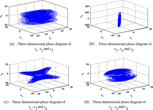
The state variables of Hyper-chaotic system and three-dimensional phase diagram are shown respectively in (Figures 1 and 2):

Figure 1. State variables of Hyper-chaotic system Equation (49).

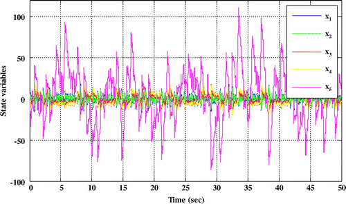
Figure 2. Three-dimensional phase diagram of Hyper-chaotic system Equation (49).

5.2. Simulations of the systems with the uncertainty and disturbance in the input matrix

In this section, the system uncertainty has in the input matrix B(x,θ) and $\theta \in [0,20]$. Where θ and w(x,t) are uncertainty and external disturbance, respectively.(50) $$\left\{\begin{array}{c}\left[\begin{array}{c}{\dot{x}}_1\\ \begin{array}{c}{\dot{x}}_2\\ {\dot{x}}_3\\ {\dot{x}}_4\\ {\dot{x}}_5\end{array}\end{array}\right]=\left[\begin{array}{ccccc}-a& a+x_3{x}_4& 0& 0& 0\\ b-x_3{x}_4& b& 0& 0& 1\\ x_2{x}_4& -c& -d& -e& 0\\ x_2{x}_3& 0& 0& -f& 0\\ -g& -g& 0& 0& 0\end{array}\right]\left[\begin{array}{c}\begin{array}{c}{x}_1\\ x_2\end{array}\\ x_3\\ x_4\\ x_5\end{array}\right]+\left[\begin{array}{c}0\\ 0\\ 0\\ 0\\ 1+\theta \end{array}\right]u+\left[\begin{array}{c}0\\ 0\\ 0\\ 0\\ 1\end{array}\right]w(x,t)\hfill \\ w(x,t)=0.1e^{-t}sin(\pi x_5)\hfill \\ x_0={\left[\begin{array}{ccc}-2& 1.5& \begin{array}{cc}1& \begin{array}{cc}0& 2\end{array}\end{array}\end{array}\right]}^T\hfill \end{array}\right.$$(50) (51) $$Q=\left[\begin{array}{ccccc}1& 0& 0& 0& 0\\ 0& 1& 0& 0& 0\\ 0& 0& 1& 0& 0\\ 0& 0& 0& 1& 0\\ 0& 0& 0& 0& 1\end{array}\right],R=[1].$$(51)

After applying the methods of ROC and GROSMC, behaviors of the state variables are simulated and they are compared together in (Figures 3 ^{Figure 4 Figure 5 Figure 6}–7):

Figure 3. Comparison of time responses x ₁in the two methods while uncertainty and disturbance in the input matrix.

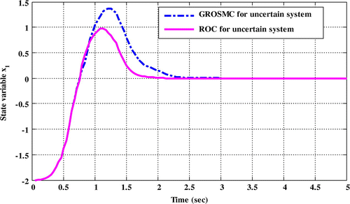
Figure 4. Comparison of time responses x ₂ in the two methods while uncertainty and disturbance in the input matrix.

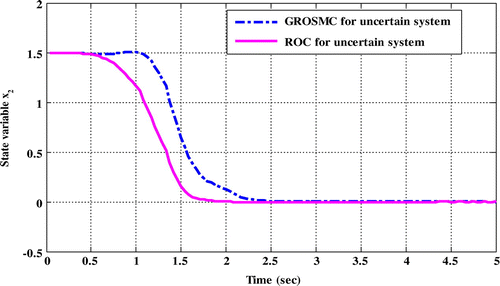
Figure 5. Comparison of time responses x ₃ in the two methods while uncertainty and disturbance in the input matrix.

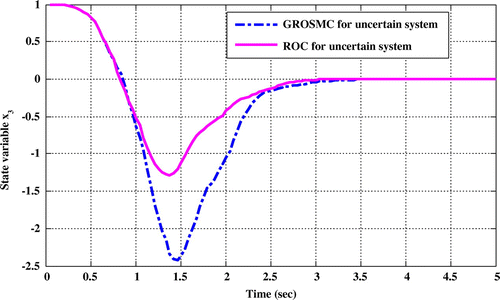
Figure 6. Comparison of time responses x ₄ in the two methods while uncertainty and disturbance in the input matrix.

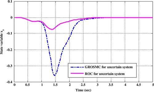
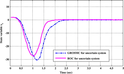
Figure 7. Comparison of time responses x ₅ in the two methods while uncertainty and disturbance in the input matrix.

5.3. Simulations of the systems with the uncertainty in the state matrix

In this section, the system uncertainty has in the state matrix A(x,θ). Where θ is uncertainty in the system and $\theta \in [0,40]$.(52) $$\left\{\begin{array}{c}\left[\begin{array}{c}{\dot{x}}_1\\ \begin{array}{c}{\dot{x}}_2\\ {\dot{x}}_3\\ {\dot{x}}_4\\ {\dot{x}}_5\end{array}\end{array}\right]=\left[\begin{array}{ccccc}-a& a+x_3{x}_4& 0& 0& 0\\ b-x_3{x}_4& b& 0& 0& 1\\ x_2{x}_4& -c& -d& -e& 0\\ x_2{x}_3& 0& 0& -f& 0\\ -g& -g& 0& 0& \theta \end{array}\right]\left[\begin{array}{c}\begin{array}{c}{x}_1\\ x_2\end{array}\\ x_3\\ x_4\\ x_5\end{array}\right]+\left[\begin{array}{c}0\\ 0\\ 0\\ 0\\ 1\end{array}\right]u+\left[\begin{array}{c}0\\ 0\\ 0\\ 0\\ 1\end{array}\right]w(x,t)\hfill \\ w(x,t)=0.1e^{-t}sin(\pi x_5)\hfill \\ x_0={\left[\begin{array}{ccc}-2& 1.5& \begin{array}{cc}1& \begin{array}{cc}0& 2\end{array}\end{array}\end{array}\right]}^T\hfill \end{array}\right.$$(52)

The state matrix is analyzed as follows:(53) $$\left[\begin{array}{ccccc}-a& a+x_3{x}_4& 0& 0& 0\\ b-x_3{x}_4& b& 0& 0& 1\\ x_2{x}_4& -c& -d& -e& 0\\ x_2{x}_3& 0& 0& -f& 0\\ -g& -g& 0& 0& \theta \end{array}\right]-\left[\begin{array}{ccccc}-a& a+x_3{x}_4& 0& 0& 0\\ b-x_3{x}_4& b& 0& 0& 1\\ x_2{x}_4& -c& -d& -e& 0\\ x_2{x}_3& 0& 0& -f& 0\\ -g& -g& 0& 0& 0\end{array}\right]=\left[\begin{array}{c}0\\ 0\\ 0\\ 0\\ 1\end{array}\right]\varphi (\theta )=B\varphi (\theta )$$(53)

where matrix ϕ(θ) is limited and it is composed as follows:(54) $$\varphi (\theta )=\left[\begin{array}{ccccc}0& 0& 0& 0& \theta \end{array}\right]$$(54)

The uncertain system Equation (52) is rewritten as follows:(55) $$\left\{\begin{array}{c}\left[\begin{array}{c}{\dot{x}}_1\\ \begin{array}{c}{\dot{x}}_2\\ {\dot{x}}_3\\ {\dot{x}}_4\\ {\dot{x}}_5\end{array}\end{array}\right]=\left[\begin{array}{ccccc}-a& a+x_3{x}_4& 0& 0& 0\\ b-x_3{x}_4& b& 0& 0& 1\\ x_2{x}_4& -c& -d& -e& 0\\ x_2{x}_3& 0& 0& -f& 0\\ -g& -g& 0& 0& 0\end{array}\right]\left[\begin{array}{c}\begin{array}{c}{x}_1\\ x_2\end{array}\\ x_3\\ x_4\\ x_5\end{array}\right]+\left[\begin{array}{c}0\\ 0\\ 0\\ 0\\ 1\end{array}\right]u+B\varphi (\theta )\left[\begin{array}{c}\begin{array}{c}{x}_1\\ x_2\end{array}\\ x_3\\ x_4\\ x_5\end{array}\right]+\left[\begin{array}{c}0\\ 0\\ 0\\ 0\\ 1\end{array}\right]0.1e^{-t}sin(\pi x_5)\hfill \\ x_0={\left[\begin{array}{ccc}-2& 1.5& \begin{array}{cc}1& \begin{array}{cc}0& 2\end{array}\end{array}\end{array}\right]}^T\hfill \end{array}\right.$$(55) (56) $${\varphi }^T(\theta )\varphi (\theta )\le F\to \left[\begin{array}{ccccc}0& 0& 0& 0& 0\\ 0& 0& 0& 0& 0\\ 0& 0& 0& 0& 0\\ 0& 0& 0& 0& 0\\ 0& 0& 0& 0& {\theta }^2\end{array}\right]\le \left[\begin{array}{ccccc}0& 0& 0& 0& 0\\ 0& 0& 0& 0& 0\\ 0& 0& 0& 0& 0\\ 0& 0& 0& 0& 0\\ 0& 0& 0& 0& 1600\end{array}\right]$$(56) (57) $$Q=\left[\begin{array}{ccccc}1& 0& 0& 0& 0\\ 0& 1& 0& 0& 0\\ 0& 0& 1& 0& 0\\ 0& 0& 0& 1& 0\\ 0& 0& 0& 0& 1\end{array}\right],F=\left[\begin{array}{ccccc}0& 0& 0& 0& 0\\ 0& 0& 0& 0& 0\\ 0& 0& 0& 0& 0\\ 0& 0& 0& 0& 0\\ 0& 0& 0& 0& 1600\end{array}\right]\text{and}R=[1]$$(57)

After applying the methods of ROC and GROSMC, behaviors of the state variables are simulated and they are compared together in (Figures 8 ^{Figure 9 Figure 10 Figure 11}–12).

Figure 8. Comparison of time responses x ₁in the two methods while uncertainty in the state matrix.

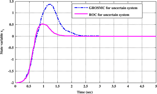
Figure 9. Comparison of time responses x ₂ in the two methods while uncertainty in the state matrix.

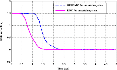
Figure 10. Comparison of time responses x ₃ in the two methods while uncertainty in the state matrix.

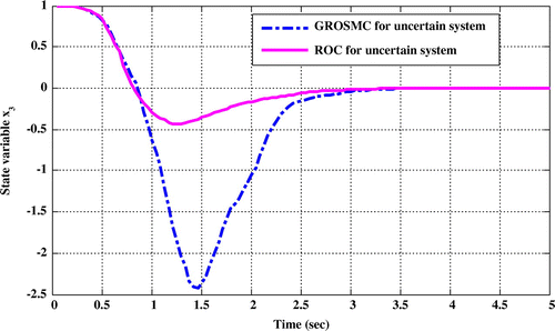
Figure 11. Comparison of time responses x ₄ in the two methods while uncertainty in the state matrix.

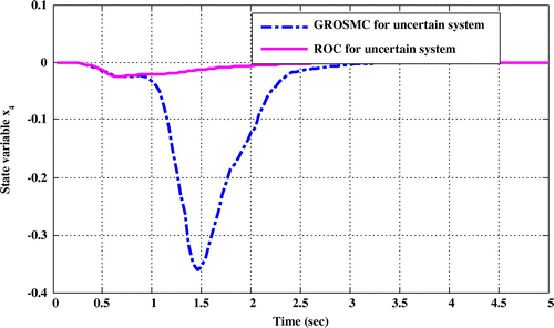
Figure 12. Comparison of time responses x ₅ in the two methods while uncertainty in the state matrix.

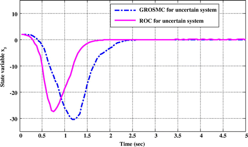
Comparing the time response of state variables shows that in ROC method, sitting time, overshoot and undershoot are lower than the GROSMC method.

6. Conclusions

In this paper, the problem of optimal control for a class of affine nonlinear systems with uncertainties and external disturbances is studied. For this purpose, the SDRE method was considered as an optimal solution and then by replacing a few simple constraints and extending the SDRE controller, the ROC controller was obtained. The simulation results show that the ROC method can be also used in the optimal control of complex systems such as Hyper-chaotic systems.

In comparison to the GROSMC method, the proposed method is not only simpler (in matching condition) and does not need to design a sliding surface (to eliminate disturbances and uncertainties), but also the characteristics of time response such as sitting time, overshoot and undershoot are lower than the GROSMC method. Thus, proposed controller’s ability in the time responses of nonlinear systems are more sufficient than the controller of the GROSMC method.

6.1. Future works

In order to expand the robust optimal controller (ROC), it is proposed to extend this method to a wider class of nonlinear systems, such as:(58) $$\dot{x}=f(x)+g(x,u)$$(58) (59) $$\dot{x}=f(x,u)$$(59)

Also, in order to enhance the time response capability, the intelligent methods can be used to optimize the weight parameters in the SDRE and the ROC methods.

Funding

The authors received no direct funding for this research.

Corrigendum

This article was originally published with errors. This version has been corrected. Please see Corrigendum (https://doi.org/10.1080/23311916.2018.1472912).

Additional information

Notes on contributors

Mohammad Khoshhal Rudposhti

Mohammad Khoshhal Rudposhti is a PhD Student in Control and System Engineering at the Department of Electrical Engineering, Science and Research branch, Islamic Azad University, Tehran, Iran. His research interests include Nonlinear Control, Optimal control, Robust control, Sliding mode control, Neural Networks Controller.

Mohammad Ali Nekoui

Mohammad Ali Nekoui an associate professor at the Faculty of Electrical Engineering, K.N.Toosi University of Technology, Tehran, Iran. His research interests include Control Engineering, Optimal control, fractional control.

Mohammad Teshnehlab

Mohammad Teshnehlab is a professor at the Faculty of Electrical Engineering, K.N.Toosi University of Technology, Tehran, Iran. His research interests include Linear Control, Linear Control, Neural Networks Controller, Knowledge and Expert Systems, Fuzzy Systems and Control, Evolutionary optimization, Soft Computing (Neural-Fuzzy Networks , Genetic Algorithms), Advanced Artificial Intelligence.

References

- Abagnale, C. , Aggogeri, F. , Borboni, A. , Strano, S. , & Terzo, M. (2017). Dead-zone effect on the performance of state estimators for hydraulic actuators. Meccanica , 52 (9), 2189–2199.10.1007/s11012-016-0563-3
- Acarman, T. (2009). Nonlinear optimal integrated vehicle control using individual braking torque and steering angle with on-line control allocation by using state-dependent Riccati equation technique. Vehicle System Dynamics , 47 (2), 155–177.10.1080/00423110801932670
- Beeler, S. C. , Tran, H. T. , & Banks, H. T. (2000a). State estimation and tracking control of nonlinear dynamical systems . Raleigh, NC: North Carolina State University at Raleigh Departmentt of Mathematics.10.21236/ADA453162
- Beeler, S. C. , Tran, H. T. , & Banks, H. T. (2000b). Feedback control methodologies for nonlinear systems. Journal of Optimization Theory and Applications , 107 (1), 1–33.10.1023/A:1004607114958
- Beikzadeh, H. , & Taghirad, H. R. (2011). Exponential nonlinear observer design based on differential state-dependent riccati equation. Journal of Control , 4 (4), 14–23.
- Beikzadeh, H. , & Taghirad, H. D. (2012). Exponential nonlinear observer based on the differential state-dependent Riccati equation. International Journal of Automation and Computing , 9 (4), 358–368.10.1007/s11633-012-0656-y
- Burghart, J. (1969). A technique for suboptimal feedback control of nonlinear systems. IEEE Transactions on Automatic Control , 14 (5), 530–533.10.1109/TAC.1969.1099251
- Choi, H. H. (2012). SDRE-based near optimal nonlinear controller design for unified chaotic systems. Nonlinear Dynamics , 70 (3), 2063–2070.10.1007/s11071-012-0598-5
- Gao, Z. , Gao, B. , Mu, D. , & Gao, S. (2016). Robust adaptive SDRE filter and its application to SINS/SAR integration. Proceedings – 2016 3rd International Conference on Information Science and Control Engineering, ICISCE, art No. 7726397, 1408–1412.10.1109/ICISCE.2016.300
- Gao, Y. , Wang, Y. , & Cheng, W. (2017). Nonlinear robust adaptively SDRE filtering method for SINS/SAR integrated Navigation SystemCGNCC 2016. 2016 IEEE Chinese Guidance, Navigation and Control Conference, Art No. 7829165 , 2383–2387.
- Garrard, W. L. , McClamroch, N. H. , & Clark, L. G. (1967). An approach to sub-optimal feedback control of non-linear systems. International Journal of Control , 5 (5), 425–435.10.1080/00207176708921775
- Khaloozadeh, H. , & Abdolahi, A. (2004, January). A new iterative procedure for optimal nonlinear regulation problem. In Proceedings of the 3rd International Conference on System Identification and Control Problems (SICPRO) (pp. 1256–1266).
- Krikelis, N. J. , & Kiriakidis, K. I. (1992). Optimal feedback control of non-linear systems. International Journal of Systems Science , 23 (12), 2141–2153.10.1080/00207729208949445
- Kumar, E. V. , Jerome, J. , & Raaja, G. (2014). State dependent Riccati equation based nonlinear controller design for ball and beam system. Procedia Engineering , 97 , 1896–1905.10.1016/j.proeng.2014.12.343
- Liccardo, F. , Strano, S. , & Terzo, M. (2013). Optimal Control Using State-dependent Riccati Equation (SDRE) for a Hydraulic Actuator. Proceedings of the World Congress on Engineering , 3 .
- Lin, F. (2007). Robust control design: An optimal control approach (Vol. 18). Hoboken, NJ: John Wiley & Sons.10.1002/9780470059579
- Nemra, A. , & Aouf, N. (2010). Robust INS/GPS sensor fusion for UAV localization using SDRE nonlinear filtering. IEEE Sensors Journal , 10 (4), 789–798.10.1109/JSEN.2009.2034730
- Pang, H. , & Wang, L. (2009, October). Global robust optimal sliding mode control for a class of affine nonlinear systems with uncertainties based on SDRE. In Computer Science and Engineering, 2009. WCSE’09. Second International Workshop on (Vol. 2, pp. 276–280). Qingdao: IEEE.10.1109/WCSE.2009.812
- Parrish, D. K. , & Ridgely, D. B. (1997, June). Attitude control of a satellite using the SDRE method. In American Control Conference, 1997. Proceedings of the 1997 (Vol. 2, pp. 942–946). IEEE.
- Pearson, J. D. (1962). Approximation methods in optimal control I. Sub-optimal control. International Journal of Electronics , 13 (5), 453–469.10.1080/00207216208937454
- Pukdeboon, C. (2015). Inverse optimal sliding mode control of spacecraft with coupled translation and attitude dynamics. International Journal of Systems Science , 46 (13), 2421–2438.10.1080/00207721.2015.1011251
- Pukdeboon, C. , & Zinober, A. S. I. (2009a). Optimal sliding mode controllers for attitude tracking of spacecraft. Paper presented at the Control Applications,(CCA) & Intelligent Control,(ISIC), 2009 IEEE.
- Pukdeboon, C. , & Zinober, A. S. I. (2009b, July). Optimal sliding mode controllers for attitude tracking of spacecraft. In Control Applications,(CCA) & Intelligent Control,(ISIC), 2009 IEEE (pp. 1708–1713). IEEE.
- Salamci, M. U. , & Gökbilen, B. (2007). SDRE missile autopilot design using sliding mode control with moving sliding surfaces. IFAC Proceedings Volumes , 40 (7), 768–773.10.3182/20070625-5-FR-2916.00131
- Strano, S. , & Terzo, M. (2015). A SDRE-based tracking control for a hydraulic actuation system. Mechanical Systems and Signal Processing , 60 , 715–726.10.1016/j.ymssp.2015.01.027
- Strano, S. , & Terzo, M. (2016). Accurate state estimation for a hydraulic actuator via a SDRE nonlinear filter. Mechanical Systems and Signal Processing , 75 , 576–588.10.1016/j.ymssp.2015.12.002
- Strano, S. , & Terzo, M. (2017). Vehicle sideslip angle estimation via a Riccati equation based nonlinear filter. Meccanica , 52 (15), 3513–3529.10.1007/s11012-017-0658-5
- Wang, X. , Yaz, E. E. , & Long, J. (2014). Robust and resilient state-dependent control of continuous-time nonlinear systems with general performance criteria. Systems Science & Control Engineering: An Open Access Journal , 2 (1), 34–40.10.1080/21642583.2013.877859
- Wernli, A. , & Cook, G. (1975). Suboptimal control for the nonlinear quadratic regulator problem. Automatica , 11 (1), 75–84.10.1016/0005-1098(75)90010-2
- Yuan, H. M. , Liu, Y. , Lin, T. , Hu, T. , & Gong, L. H. (2017). A new parallel image cryptosystem based on 5D hyper-chaotic system. Signal Processing: Image Communication , 52 , 87–96.