Bi-objective evolutionary optimization of level of service in urban transportation based on traffic density

Abstract

This work investigates levels of service in urban transportation coupling a multi-objective evolutionary algorithm with the multi-agent traffic simulator MATSim. The evolutionary algorithm searches combinations of the number of private/public transportation users, capacity of buses, and time interval between bus departures minimizing traffic density and travel time simultaneously. MATSim simulates the movement of 27,000 agents according to the solutions of the evolutionary algorithm on a model of the traffic network of Quito city. We study the trade-off in objectives and analyze the solutions produced to gain knowledge about the conditions to achieve different levels of service. Also, we analyze fuel consumption and particulate matter emissions for the trade-off solutions. This work is useful for decision makers to suggest policies that can improve mobility combining private and public transportation.

Keywords:

• level of service
• multi-objective optimization
• evolutionary computing
• sustainable transport systems

Public Interest Statement

Approximately half of the world population currently lives in metropolitan areas, and for 2050 the projections show that will increase to two-thirds. The people’s mobilization demands traffic infrastructure and public transportation that does not grow at the same pace as the population, which cause problems like congestion and pollution. In this work, we simulate the movement of 27,000 agents on a model of the traffic network of Quito city to investigate levels of service in urban transportation coupling a multi-objective evolutionary algorithm with the multi-agent traffic simulator MATSim. The evolutionary algorithm searches combinations of the number of private/public transportation users, capacity of buses, and time interval between bus departures minimizing traffic density and travel time simultaneously. We study the trade-off in objectives and analyze fuel consumption and particulate matter emissions of the trade-off solutions which assists to the decision makers for suggest policies that can improve mobility combining private and public transportation.

1. Introduction

Figure 15. PM emission difference between A8b and A8a.

Currently, around 54% of the world’s population lives in urban areas. The world’s population is expected to grow in the future and the proportion of the urban population as well. By 2050, the urban population is projected to increase to 66% (United Nations & Social Affairs, 2014). Population growth and urbanization trends have increased the demand for urban transportation and will continue to do so in the future. Often, existent traffic infrastructure and public transportation systems cannot cope with the increasing demand. Thus, dwellers tend to use their private means of transportation. Particularly, in emerging large cities, where the public transportation has not been able to satisfy the demand, the number of vehicles is increasing considerably and rendering mobility problems even worse (Gakenheimer, 1999). Congestion and delays add substantial costs that could be avoided, increases pollution and the risk of accidents.

The design optimization of urban transportation systems is a complex problem with multiple interrelated components that impose a continuous challenge for city planners. Evolutionary algorithms (EAs) and other heuristics have proved effective to optimize difficult problems and are being investigated in the mobility and transportation domain. Some applications of single and multi-objective EAs to road network design, bus network optimization, and public transportation routing scheduling are as follows. In an early work (Bielli, Caramia, & Carotenuto, 2002), the authors use a single-objective genetic algorithm (GA) for bus network optimization. Hee, Kyung, and Hyuk (2012) solve a road network design problem (RNDP) using a bi-level optimization approach that reflects the different objectives between planners and network users. They focused on the design of a small network with six links and six nodes using a multi-objective GA and optimizing three objectives related to travel time, fuel consumption, and accessibility to network’s nodes. Other works focus on public transportation routing and scheduling. Arbex and da Cunha (2015) use a bi-objective approach to minimize both passengers and operators costs on a benchmark network (15 nodes and 21 links). Ma et al. (2017) studied stop selection, line planning, and timetables for customized bus (CB). They used a single-objective GA to solve a weighted fitness function considering passenger, operator, and societal perspectives and test their model on real network areas that cover 3$k{m}^2$ and 18$k{m}^2$. Other works focusing on frequency setting and vehicle scheduling problem employee GAs and a bi-level approach. Regarding frequency setting problem, in Yu, Yang, and Yao (2010), at the upper level, the frequency routes are optimized minimizing the passenger’s travel time meanwhile in the lower level an assignation of transit trips to bus optimal route strategy is set. A single-objective GA is implemented to search the frequency of each route. The results obtained show that the optimal solution can decrease total travel time by about 6% compared with the current situation. They used a heuristic where the optimal strategy and the expected total travel time from each node to the destination node are computed, and the demand is assigned to the network according to the optimal strategy from all origins to the destination. In another study (Verbas & Mahmassani, 2015), the authors propose a bi-level model where at the upper level a frequency setting problem is addressed minimizing waiting times and use a heuristic model running a simulation at the lower level according to a demand and frequency. Both previous works used one pre-defined demand, a macro-model, and simulation schema to study the effects of a frequency setting in travel time and waiting time, respectively. Regarding scheduling problems, in Farhan Ahmad (2005), the authors state a bi-level approach to solve a bus scheduling problem for overlapping routes. In the first level, the model minimizes the number of buses required for each route individually and considering load feasibility. In the second level, given the fleet size computed in the first level, the fleet size is minimized again by considering all routes together by using a single-objective GA. They tested the model in a real-world network with a total of 60 nodes and 70 links. Link distance in time units and symmetric demand matrix gives the evaluation of each solution. The results showed that the reduction in fleet size is not significant as it was expected during model formulation stage due to little overlapping of routes in the test network.

In this work, we study the urban transportation system under various proportions of private and public transportation users, aiming to understand the conditions to achieve different levels of service and their implications on the optimal configuration of the public transportation, fuel consumption (energy), and the impact on the environment.

The level of service (LoS) is a quality measure describing operational conditions within a traffic stream, generally in terms of service measures such as speed and travel time, freedom of maneuver, traffic interruptions, and comfort and convenience (Board, 2000). In this work, we define LoS in terms of traffic density, which is determined by the total number of vehicles that circulate in the city given by the proportions of the population that use public and private transportation.

To make public transportation more attractive, city planners need to guarantee a reliable service with appropriate frequency and capacity of buses to satisfy the mobility demand. For a given proportion of public transportation users, we should find a proper configuration of bus capacities and departure times between buses. Different proportion and configurations will impact travel time, fuel consumption, costs, and emissions, in addition to traffic density. Most of these criteria are in conflict with each other. For example, the transportation service administration would like to maximize the use of the infrastructure minimizing costs and energy. Increasing the frequency of buses can increase the capacity of the system. However, this could carry additional costs. Users would like to minimize their travel times. This could be an incentive to use private transportation but could increase their costs. In addition, people living in zones where there are public transportation routes would like to minimize emissions or pollution. A way to improve the flow is reducing the volumeof traffic or density. However, reducing density has impacts in the total travel time of the users because they need to use public transportation. These trade-offs suggest that compromised solutions can be found using a multi-objective optimization approach.

We use a multi-objective EA to search combinations of number of private/public transportation users, capacity of buses, and time interval between bus departures, minimizing traffic density and travel time simultaneously. In order to have a broad vision of the possible solutions to the problem and their LoS, at this time we assume that buses are always available in different capacities, do not constraint their total number, and do not consider cost.

We conduct our study using a scenario based on a real traffic network from Quito city (Ecuador). Quito’s population has grown considerably in the last years. Currently, its urban transportation system is highly congested due to an increase of private vehicles combined with a poorly satisfied demand by public transportation. It is important to find alternative configurations of the urban transportation system to improve the LoS and quality of life in the city. In this work, we model the mobility of 27,000 agents that use private and public transportation on an area of 40$k{m}^2$, and simulate their mobility using MATSim (Horni, Nagel, & Axhausen, 2016), a multi-agent transport simulator.

The rest of this paper is organized as follows. In the next section, we describe the design optimization approach we follow, the problem formulation, and the simulation of mobility. In Section 3, we describe the EA, mainly its representation, operators, and fitness functions. Section 4 is devoted to simulation results and discussion. Finally, in Section 5, conclusions and future work are presented.

2. Method

2.1. Components and overview

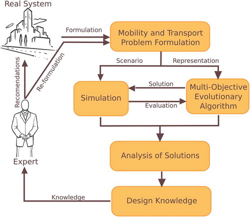
We follow the design optimization approach illustrated in Figure 1. We first formulate the bi-objective optimization of LoS in urban transportation based on transit density, simulate the urban transportation in the city using a specialized transport simulator. We use a multi-objective EA to find optimal solutions to the formulated problem evaluating the quality of solutions using the outcome of the simulation, analyze the solutions produced by the EA, and extract knowledge about the system. The approach is iterative, where the solutions and obtained knowledge are made available to the expert for further analysis. The feedback from the expert could be used to reformulate the problem to study additional details. Once the expert is satisfied, the knowledge gained could be suggested to improve the real system.

Figure 1. Method.

2.2. Problem definition

Given a total fixed number of travelers that can use either public or private transportation, a number of bus lines and a set of schedule periods, the problem consists in finding optimal configurations of the public transportation system in terms of bus capacities and headways (time between bus departures in the same line) for a range of proportions of public transportation users minimizing simultaneously travel time and traffic density.

The problem is formulated as follows:

$\begin{array}{cccc}\hspace{0.17em}& \mathrm{m}\mathrm{i}\mathrm{n}\mathrm{i}\mathrm{m}\mathrm{i}\mathrm{z}\mathrm{e}& \hspace{0.17em}& \mathbf{f}(\mathbf{x})=(f_1(\mathbf{x}),f_2(\mathbf{x}))\\ \hspace{0.17em}& \mathrm{s}\mathrm{u}\mathrm{b}\mathrm{j}\mathrm{e}\mathrm{c}\mathrm{t}\mathrm{t}\mathrm{o}& \hspace{0.17em}& \hspace{0.17em}\\ \hspace{0.17em}& \hspace{0.17em}& \hspace{0.17em}& \mathbf{x}=(n_{Pc},n_{Pt},\mathbf{c},\mathbf{h})\\ \hspace{0.17em}& \hspace{0.17em}& \hspace{0.17em}& n_A=n_{Pc}+n_{Pt}\\ \hspace{0.17em}& \hspace{0.17em}& \hspace{0.17em}& 0.2n_A<n_{Pt}<0.8n_A\\ \hspace{0.17em}& \hspace{0.17em}& \hspace{0.17em}& \mathbf{c}=\{c_i^j\in C\},i=1,\cdots ,n_B\mathrm{a}\mathrm{n}\mathrm{d}j=1,\cdots ,n_S\\ \hspace{0.17em}& \hspace{0.17em}& \hspace{0.17em}& \mathbf{h}=\{h_i^j\in H\},i=1,\cdots ,n_B\mathrm{a}\mathrm{n}\mathrm{d}j=1,\cdots ,n_S\\ \hspace{0.17em}& \hspace{0.17em}& \hspace{0.17em}& \hspace{0.17em}\end{array}$

Function $f_1(\mathbf{x})$ measures travel time of all travelers and function $f_2(\mathbf{x})$ measures the traffic density, $\mathbf{x}$ is the vector of decision variables, $n_{Pc}$ is number of private transportation travelers, $n_{Pt}$ is the number of public transportation users, $c_i^j$ is the capacity (maximum number of passengers) of the buses assigned to line i at schedule period j, $n_B$ is the number of bus lines, $n_S$ is the number of schedule periods, $\mathbf{c}$ is the vector of capacities associated to all bus lines and schedule periods, $h_i^j$ is the headway departure or time between departure of buses on line $i$ for schedule period $j$, $\mathbf{h}$ is the vector of headways associated to all bus lines and schedule periods, C is a finite set of bus capacities, and H is a finite set of headways expressed in minutes.

2.3. Area of study

We study the conditions to achieve different levels of service in Quito city (Ecuador). The geographical area of study includes the central zone of the city, where several universities, big malls, two parks, a stadium, and the main hub of the private and public transportation infrastructure are located. The area of study also includes residential zones and the business district. The total area represents approximately 40km². Figure 2 shows the extension of the geographical area.

Figure 2. DMQ BRT scenario.

The population in Quito was around 2 million in 2010 (INEC, 2010), of which 80% move every day to accomplish various activities. Main mobility reasons according to DMQ (2012) are 31% for work, 32.5% for study (all educational levels), and 36.5% for other different activities. It is estimated that 47% of traffic flows go to the zone we study in this work (GrupoFaro, 2010). From this percentage, 74.5% use public transportation and 25.5% private cars. In our study, we simulate a sample of 27.000 agents.

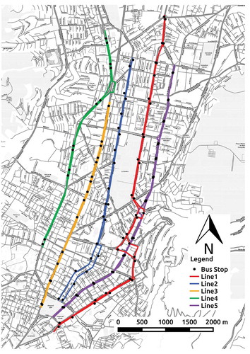
The massive passenger transportation in Quito is performed by private and public companies. The Passenger Transportation Metropolitan Company is a public company in charge of the Bus Rapid Transit (BRT) service. In 2015, approximately 650,000 passengers were transported daily by the different BRT lines (DMQ, 2015). In our model, we consider five main BRT corridors (see Figure 2) which are the most demanded and congested routes.

2.4. Simulation

In this work, we use MATSim, an agent-based transport simulation framework (Horni et al., 2016). It performs a micro-simulation of agents that move on a transportation system producing information about agent routes and movements. MATSim requires as inputs the model of the transport network infrastructure, public transportation configuration, and the agents’ mobility plans.

The network comes from Geofabrik and OpenStreetMap (Frederik, Topf, & Karch, 2007). The number of links of the network corresponding to the area of study is 8192. The links’ attributes are length (m), flow capacity that defines how many cars can pass through the road during a unit of time, e.g., vehicles/hour, and free speed that represents the maximum flow velocity. For this work, we take into account all the main and secondary pathways with free speeds equal or above 30 km/h.

Figure 3 shows the integration between the simulator and the EA. The EA searches optimal settings for capacity and headway bus line configuration for a given proportion of agents that will use public transportation.

Figure 3. Simulation and EA integration.

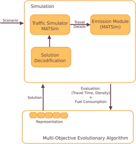
To evaluate a solution, MATSim sets the bus line capacities and headways with the solution provided by the optimizer, computes the routes of the agents based on heuristics, and simulates the mobility of all agents (private and public transportation) following their mobility plans. MATSim simulates the public transportation by setting stop locations, lines, schedule, routes, departures, and vehicles. A line consists of two or more routes defined over the network links and a list of departure times with a reference to a particular bus specification (e.g., capacity, length, technology) (Horni et al., 2016). MATSim emission module (Hülsmann, Gerike, Benjamin, Nagel, & Luz, 2011) computes the fuel consumption and emissions for cars and buses by connecting MATSim output to comprehensive database Handbook on Emission Factors for Road Transportation (HBEFA) (Keller & Wuthrich, 2014). The output collected from the simulator is used to calculate travel time and traffic density, which are passed back to the optimizer as objective values to compute the fitness of the solution.

3. Evolutionary algorithm

This section explains the representation, algorithm, operators, and fitness functions that are used in this study.

3.1. Solution representation

In this work, we consider private cars and city buses as the only means of private and public transportation, respectively. The main components of our representation are the number of travelers that use public transportation $n_{Pt}$ and the bus lines configurations given by capacities c and headways h. In this work $n_{Pt}$ can take values in the range [0.2$n_A$, 0.8$n_A$] in intervals of 0.1$n_A$, where $n_A$ is the total number of travelers or agents. The number of private transportation travelers is $n_{Pc}=n_A-n_{Pt}$. 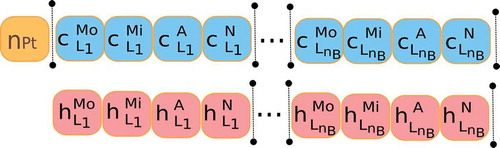The $n_B$ bus lines are identified by the set of indexes $L=\left\{L_1,\cdots ,L_{n_B}\right\}$ and the $n_S$ schedule periods by the set of indexes $S=\left\{M_o,M_i,A,N\right\}$ for morning, midday, afternoon, and night. A solution for the EA is represented by the following integer variables:

(1) $\left(n_{Pt},\mathbf{c},\mathbf{h}\right),$(1)

where

(2) $\begin{array}{rl}& \mathbf{c}=\left\{c_i^j\in C\right\},i=1,\cdots ,n_B\mathrm{a}\mathrm{n}\mathrm{d}j=1,\cdots ,n_S\\ & \mathbf{c}=\left\{c_{L_1}^{M_o},\cdots ,c_{L_1}^N,\cdots ,c_{L_{n_B}}^{M_o},\cdots ,c_{L_{n_B}}^N\right\}\end{array}$(2)

(3) $\begin{array}{rl}& \mathbf{h}=\left\{h_i^j\in H\right\},i=1,\cdots ,n_B\mathrm{a}\mathrm{n}\mathrm{d}j=1,\cdots ,n_S\\ & \mathbf{h}=\left\{h_{L_1}^{M_o},\cdots ,h_{L_1}^N,\cdots ,h_{L_{n_B}}^{M_o},\cdots ,h_{L_{n_B}}^N\right\}\end{array}$(3)

Here, $c_i^j$ is the capacity of bus (number of passengers) of line i for schedule period j, $c_i^j\in C=\left\{0,1,2\right\}$ where 0, 1, and 2 denote small, medium, and large capacity, respectively. $h_i^j$ is the headway departure or time between departure of buses on line $i$ for schedule period $j$. $h_i^j\in H=\left\{0,1,\cdots ,11\right\}$, to represent headways from 5 to 60 min in steps of 5. Figure 4 illustrates the representation of solutions used by the EA.

Figure 4. Solution representation.

3.2. Adaptive $\epsilon$-Sampling and $v$-Hood (A $\epsilon S$ $vH$ ) algorithm

In this section, we explain the proposed A$\epsilon S$ $vH$ algorithm, an extension of the multi- and many-objective (A$\epsilon$S$\epsilon$H) algorithm (Aguirre, Oyama, & Tanaka, 2013; Aguirre, Yazawa, Oyama, & Tanaka, 2014). The proposed A$\epsilon S$ $vH$ creates neighborhoods in variable space to bias mating for recombination and uses $\epsilon$-dominance principles to truncate the population when the number of non-dominated solutions is larger than the population size.

Procedure 1 A ε SvH

Require: Population size P _size

Ensure: ${\mathcal{F}}_1$, set of Pareto non-dominated solutions

1: ${\epsilon }_s\leftarrow 0$, ${\mathrm{\Delta }}_s\leftarrow {\mathrm{\Delta }}_0$//set ${\epsilon }_s$-dominance factor and its step of adaptation

2: $\mathcal{P}$ random//initial population $\mathcal{P}$, $|\mathcal{P}|=P_{size}$

3: evaluation($\mathcal{P}$)

4: repeat

5://Parent selection

6: $\left\{\mathcal{H},N_H\right\}\leftarrow$ $v$-hood creation ($\mathcal{P}$) $\mathcal{H}=\left\{{\mathcal{H}}_j\right\},j=1,2,\cdots ,N_H$

7: ${\mathcal{P}}^{\prime }\leftarrow$ $v$-hood mating($\mathcal{H}$, $Psize$)

8://Offspring creation

9: $\mathcal{Q}\leftarrow$recombination and mutation (${\mathcal{P}}^{\prime }$)//$|\mathcal{Q}|=|\mathcal{P}|=P_{size}$

10://Evaluation and front sorting

11: evaluation($\mathcal{Q}$)

12: $\mathcal{F}\leftarrow$ non-dominated sorting ($\mathcal{P}\cup \mathcal{Q}$)//$\mathcal{F}=\left\{{\mathcal{F}}_i\right\},i=1,2,\cdots ,N_F$

13://Survival selection

14: $\{\mathcal{P},N_S\}\leftarrow$ $\epsilon$-sampling truncation ($\mathcal{F}$, ${\epsilon }_s$, $P_{size}$) $N_S$, number of samples

15: $\left\{{\epsilon }_s,{\mathrm{\Delta }}_s\right\}\leftarrow$ adapt (${\epsilon }_s$, ${\mathrm{\Delta }}_s$, $P_{size}$, $N_S$)

16: until termination criterion is met

17: return ${\mathcal{F}}_1$

The algorithm’s flow is illustrated in Procedure 1. It starts by setting initial default values for the parameter ${\epsilon }_s$ used in and its step of adaptation ${\mathrm{\Delta }}_s$. The population $\mathcal{P}$ is randomly initialized and evaluated. The main loop starts by creating neighborhoods of solutions, grouping them by proximity in variable space using a $v$-hood creation procedure. Next, $v$-hood mating creates a pool of mates ${\mathcal{P}}^{\prime }$ selecting them from the same neighborhood. The selected mates are recombined and mutated to create the offspring population $\mathcal{Q}$. Since mates come from the same neighborhood, a solution would recombine only with a solution that is close by in decision space. After offspring $\mathcal{Q}$ is evaluated, non-dominated sorting is performed on the population that results from joining the current population $\mathcal{P}$ and its offspring $\mathcal{Q}$. The population of size 2$P_{size}$ sorted in non-dominated fronts $\mathcal{F}$ is then truncated to obtain the surviving population $\mathcal{P}$ of size $P_{size}$ using a $\epsilon$-sampling truncation procedure set with parameter ${\epsilon }_s$. The parameter ${\epsilon }_s$ and its step of adaptation ${\mathrm{\Delta }}_s$ are adapted every generation so that the number of $\epsilon$-sampled solutions approach the size of the population. In the following we explain with more detail $v$-hood creation, $v$-hood mating and $\epsilon$-sampling truncation.

The $v$-hood creation procedure splits the surviving population $\mathcal{P}$ into neighborhoods as illustrated in Procedure 2. First, this procedure randomly selects an individual $z$ from the population $\mathcal{P}$. Then, solutions in $\mathcal{P}$ with the same proportion of public transportation users as $z_{N_{Pt}}$ are grouped in $\mathcal{Y}$. Next, $z$ and $\mathcal{Y}$ are assigned to neighborhood ${\mathcal{H}}_i$ and removed from the population $\mathcal{P}$. Neighborhood creation is repeated until all solutions in $\mathcal{P}$ have been assigned to a neighborhood.

Mating for recombination is implemented by the procedure $v$-hood mating illustrated in Procedure 3. Neighborhoods are considered to be elements of a list. To select two mates, first a neighborhood from the list is specified deterministically in a round-robin schedule. Then, two individuals are selected randomly within the specified neighborhood, so that an individual will recombine with other individual that is located close by in variable $n_{Pt}$ space. Due to the round-robin schedule, the next two mates will be selected from the next neighborhood in the list. When the end of the neighborhood lists is reached, mating continues with the first neighborhood in the list. Thus, all individuals have the same probability of being selected within a specified neighborhood, but due to the round-robin scheduling individuals belonging to neighborhoods with fewer members have more recombination opportunities that those belonging to neighborhoods with more members. Once the pool of all mates ${\mathcal{P}}^{\prime }$ has been established, they are recombined and mutated according to the order they were selected during mating.

The $\epsilon$-sampling truncation (Aguirre et al., 2013) receives the sets of solutions $\mathcal{F}$ created by non-dominated sorting and selects exactly $P_{size}$ surviving solutions from them. If the number of non-dominated solutions $\left|{\mathcal{F}}_1\right|<P_{size}$, the fronts ${\mathcal{F}}_i$ are copied iteratively to $\mathcal{P}$ until the population is filled. If ${\mathcal{F}}_i$ overfills $\mathcal{P}$, the required number of solutions are selected randomly from ${\mathcal{F}}_i$ and copied to $\mathcal{P}$. On the other hand, if the number of non-dominated solutions $\left|{\mathcal{F}}_1\right|>P_{size}$, it calls $\epsilon$-sampling with parameter ${\epsilon }_s$ to get from ${\mathcal{F}}_1$ a sample of ${\epsilon }_s$ non-dominated solutions ${\mathcal{F}}_1^{\epsilon }\le {\mathcal{F}}_1$ and the set of ${\epsilon }_s$-dominated solutions ${\mathcal{D}}^{{\epsilon }_s}$. ${\mathcal{F}}_1^{\epsilon }$ is copied to $\mathcal{P}$. If $|\mathcal{P}|>P_{size}$, solutions are randomly eliminated from $\mathcal{P}$ until its size is $P_{size}$. If $|\mathcal{P}|<P_{size}$, solutions are randomly copied from the ${\epsilon }_s$-dominated solutions ${\mathcal{D}}^{{\epsilon }_s}$ to $\mathcal{P}$ until its size is $P_{size}$. The $\epsilon$ sampling procedure is done in way that the surviving population $\mathcal{P}$ always includes the extreme solutions present in ${\mathcal{F}}_1$.

Procedure 2 $\upsilon$-hood creation ($\mathcal{P}$)

Require: Population $\mathcal{P}$

Ensure: Neighborhoods $\mathcal{H}=\left\{{\mathcal{H}}_i\right\}$,$i=1,2,\cdots ,N_H$

1: $\mathcal{H}\leftarrow \mathrm{\varnothing }$

2: $i\leftarrow 0$

3: while $\mathcal{P}\ne \mathrm{\varnothing }$ do

4: $z\leftarrow x_r\in \mathcal{P}|r=rand(1,\mathcal{P})$ // $z$, is a randomly chosen solution from list

5: $\mathcal{Y}\leftarrow \{y\in \mathcal{P}|z_{N_{Pt}}==y_{N_{Pt}}\}$ // solutions which $N_{Pt}$ variable are equal

6: $i\leftarrow i+1$

7: ${\mathcal{H}}_i\leftarrow \left\{\left\{z\right\}{\cup }^{\mathcal{Y}}\right\}$ // $z$ and its solutions form the $N_{Pt}$-hood

8: $\mathcal{H}\leftarrow \mathcal{H}{\cup }^{{\mathcal{H}}_i}$

9: $\mathcal{P}\leftarrow \mathcal{P}\mathrm{\setminus }{\mathcal{H}}_i$

10: end while

11: $N_H\leftarrow i$

12: return $\mathcal{H}$, $N_H$

Procedure 3 $\upsilon$-hood mating($\mathcal{H},P_{size}$)

Require: Neighborhoods $\mathcal{H}=\left\{{\mathcal{H}}_i\right\}$, $i=1,2,\cdots ,N_H$ and population size $P_{size}$

Ensure: Pool of mated parents $|{\mathcal{P}}^{\prime }|=2P_{size}$

1: ${\mathcal{P}}^{\prime }\leftarrow \mathrm{\varnothing }$

2: $i\leftarrow 1$

3: $j<P_{size}$

4: while $j<P_{size}$ do

5: $\{x_{r_1},x_{r_2}\in {\mathcal{H}}_i\left|r_1\wedge r_2=rand(1,\right|{\mathcal{H}}_i|),r_1\ne r_2\}$

6: $y\leftarrow tournament(x_{r_1},x_{r_2})$ // decide based on dominance rank

7: $\{x_{r_3},x_{r_4}\in {\mathcal{H}}_i\left|r_3\wedge r_4=rand(1,\right|{\mathcal{H}}_i|),r_3\ne r_4\}$

8: $z\leftarrow tournament(x_{r_3},x_{r_4})$ // decide based on dominance rank

9: ${\mathcal{P}}^{\prime }\leftarrow {\mathcal{P}}^{\prime }\cup \{y,z\}$

10: $i\leftarrow 1+(i\mathrm{m}\mathrm{o}\mathrm{d}{N}_H)$

11: $j\leftarrow j+1$

12: end while

13: return ${\mathcal{P}}^{\prime }$

The difference between the proposed A$\epsilon$S$v$H algorithm and the A$\epsilon$S$\epsilon$H is the space where neighborhoods for parent selection is performed. In A$\epsilon S$ $\epsilon H$ neighborhoods are created in objective space, whereas in A$\epsilon S$ $vH$ neighborhoods are created in decision space. Specifically, we use the variable $n_{Pt}$ to create the neighborhoods so that all solutions with the same proportion of public transportation users belong to the same neighborhood. In this way, the method allows a less-disruptive recombination compared to A$\epsilon S$ $\epsilon H$ for the problem dealt with in this work.

3.3. Operators

To create offspring we follow the representation described above and apply uniform crossover (UX) with probability $P_c$, using a mixing ratio $pCv$. For mutation, we first decide whether to mutate $n_{Pt}$ with probability $P_m^{n_{Pt}}$ or capacities and headways (c, h) with probability $1-P_m^{n_{Pt}}$. When capacities and headways are mutated, we traverse capacities and headways for all lines and schedule periods and mutate them with probability $P_m$ per variable in (c, h). The mutation operators increase or decrease randomly with equal probability the code of the variable in which operates.

3.4. Evaluation functions

The fitness functions $f_1(\mathbf{x})$ and $f_2(\mathbf{x})$ for travel time and traffic density referred in the problem definition of Section 2.2 are computed from the outcome of the simulation. In the following, we express them in terms of the data generated from the simulator.

3.4.1. Travel time $f_1$

The travel time tt is given by the total travel time of private and public transportation and expressed by

(4) $f_1(\mathbf{x})=tt=t{t}_{pc}+t{t}_{pt}$(4)

The average travel time for private (cars) is expressed by

(5) $t{t}_{pc}=\frac{1}{n_{Pc}}\sum _{i=1}^{n_{Pc}}\sum _{l=1}^L{t}_{il},$(5)

where $t_{il}$ represents the travel time on link $l$ for vehicle $i$ and $L$ is the total links of the route.

The average travel time for public transit users is computed by

(6) $t{t}_{pt}=\frac{1}{n_{Pt}}\sum _{i=1}^{n_{Pt}}{t}_i^a-t_i^d,$(6)

where $t_i^a$ represents the arrival time to its destination and $t_i^d$ is the departure time from the origin of the trip for an agent i. This time includes walking time to the bus stop, waiting time, and bus riding time.

3.4.2. Density $f_2$

One measure of the effectiveness to define levels of service is density. Density describes the proximity of vehicles to each other, which is the principal influence on freedom to maneuver. Thus, it is an appropriate descriptor of service quality (Roess, Prassas, & McShane, 2011). Density is a relationship given by $D=v$/$S$ where $v$ is the volumeor flow rate, $S$ is the average passenger-car speed (km/h) and $D$ is the density (pc/km/ln) (Roess et al., 2011). For our scenario, density is computed by

(7) $f_2(\mathbf{x})=density=\frac{N_{TripsPc}+N_{TripsPt}}{AvgSpeed}\times \frac{1}{AvgNLinks},$(7)

where $N_{TripsPc}$ and $N_{TripsPt}$ are the total number of trips of private vehicles and public transportation, respectively, computed on the routes taken by agents. AvgSpeed is the total average speed of vehicles during the scenario duration time. AvgNLinks is the average of links traversed for each agent during its trip.

4. Simulation results and discussion

4.1. Experimental setup

We optimize five BRT lines, splitting the schedule of buses in four time periods from 06h00 to 09h00, 09h00 to 16h00, 16h00 to 20h00, and 20h00 to 22h00. These correspond to the schedule periods set $S=\left\{M_o,M_i,A,N\right\}$ for morning, midday, afternoon, and night. For each schedule period, the algorithm searches appropriate capacities and headways (frequencies) of buses. Thus, the number of variables is 41, one for the proportion of public transportation users $n_{Pt}$, $5\mathrm{l}\mathrm{i}\mathrm{n}\mathrm{e}\mathrm{s}\times 4\mathrm{s}\mathrm{c}\mathrm{h}\mathrm{e}\mathrm{d}\mathrm{u}\mathrm{l}\mathrm{e}\mathrm{p}\mathrm{e}\mathrm{r}\mathrm{i}\mathrm{o}\mathrm{d}\mathrm{s}$ for capacities c and $5\mathrm{l}\mathrm{i}\mathrm{n}\mathrm{e}\mathrm{s}\times 4\mathrm{s}\mathrm{c}\mathrm{h}\mathrm{e}\mathrm{d}\mathrm{u}\mathrm{l}\mathrm{e}\mathrm{p}\mathrm{e}\mathrm{r}\mathrm{i}\mathrm{o}\mathrm{d}\mathrm{s}$ for headways h. Capacity categories for BRT vehicles are small, medium and large with 25, 70, and 115 passengers, respectively. Headway is split into 12 categories from 5 to 60 min in steps of five minutes.

For the EA, we set population size to 100 and initialize it randomly. For the operators, we set crossover rate to $Pc$ = 1.0 with mixing ratio probability $pCv$=0.3. This means that all individuals undergo uniform crossover and offspring keeps in average 70% of the variables of one parent and 30% of the other. Mutation rate $P_m^{n_{Pt}}$ is set to 0.1 to mutate $n_{Pt}$ and $1-P_m^{n_{Pt}}=0.9$ to mutate variables in (c, h). Mutation rate per variable in (c, h) is $Pm$ = 1/n, where $n=40$ is the number of variables in (c, h). Thus, in average, mutation changes the variable $n_{Pt}$ corresponding to the number of public transportation users for 10% of the population and the variables corresponding to capacity or headways of one of the bus lines for 90% of the population. We conduct 10 runs of the EA fixing the number of generations to 100. We perform the experiments on a 64 bits Rocks cluster with 12 nodes, of which nine are 6-core 2 GHz and 3 are 16-core 2.8 GHz. The population is evaluated in parallel and the evaluation of one individual takes in average 14 min.

To evaluate each solution, we run MATSim simulating the mobility of $n_A=27.000$ agents. The mobility plan for each agent consists of two main trips or legs: (1) from home to work, study, or others and (2) from work, study, or others to home. The plans are designed so that all agents move first from each home location to different points along the area of study. Those points are facility locations such as universities, workplaces, and others like malls, and parks. In their second trip, the agents move back home. The distribution of home locations, workplaces, and education facilities for the mobility plan were chosen taking into account census data and a previous mobility study (Demoraes, 2005). We prepare in advance the settings of public transportation configuration: lines, routes, and stop locations. The public transportation configuration consists of five BRT lines, 112 stop locations, and two routes per each bus line. When MATSim receives the solution proposed by the EA, i.e., a vector of values corresponding to variables ($n_{Pt}$, c, h), the agents that will use public transportation are chosen randomly with probability $n_{Pt}/n_A$. The other agents are set to use private cars. Also, the capacities and headways for the five lines are set accordingly to the values suggested by the EA.

To compute emissions, we have selected seven categories of vehicles for private and one for public transportation. Table 1 shows the distribution of vehicle categories for private transportation chosen for the scenario, which is in accordance with census transportation data (INEC, 2010) for Quito city. We assign a category of vehicle to each agent randomly following this distribution. For public transportation, we have chosen a heavy goods vehicle HGV type which weight goes from 14 to 20 tons and diesel EuroII as fuel/technology type. Vehicle characteristics enable to identify the emission factors from HBEFA database. To compute warm emissions, MATSim combines the vehicle information with the kinematic features such as speed and stop duration obtained from the simulation.

Table 1. Automobile distribution (fuel = gasoline and weight ≤ 2 Tons)

Year-Category	%	Year-Category	%
2000–2002|Euro2	24.40	2008–2010|Euro5	13.70
2002–2004|Euro3	7.80	2010–2012|Euro6	23.80
2004–2006|Euro4	12.20	2012–2014|Euro6	5.20
2006–2008|Euro4	13.00

4.2. Comparison between A $\epsilon$ S $\epsilon$ H and A $\epsilon$ S $v$ H

In this section, we compare the proposed algorithm A$\epsilon S$ $vH$ that creates neighborhoods in decision space to perform recombination with the A$\epsilon S$ $\epsilon H$ that creates neighborhoods in objective space.

First, we compute the hypervolumeof the non-dominated set of solutions at each generation to verify their evolution. The reference point to calculate the hypervolumeis fixed to the worst values in each objective, obtained from the Pareto set of non-dominated solutions found by the algorithms in all runs. Figure 5 shows box plots of the hypervolumeover the generations for the 10 runs of both algorithms. In blue we show results by A$\epsilon S$ $\epsilon H$ and in red results by A$\epsilon$S$v$H. Note that the hypervolumerapidly increases with the generations, showing that evolution is proceeding as expected. However, the hypervolumeby A$\epsilon$S$v$H is significantly larger than A$\epsilon S$ $\epsilon H$. This means that A$\epsilon$S$v$H can find sets of non-dominated solutions with better properties of convergence and diversity than A$\epsilon S$ $\epsilon H$.

Figure 5. Hyper volumeover generations.

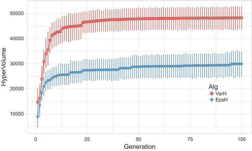
Figure 6. Hyper volumeover generations of one run.

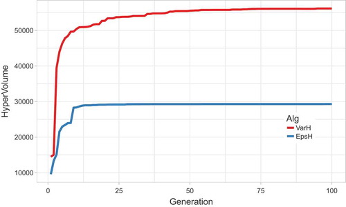
Figure 7. Pareto optimal set of one run.

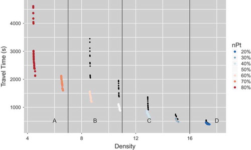
Figure 8. Travel time and density, colored by fraction of public transport users $n_{Pt}$. Black dots show POS founded by the original algorithm.

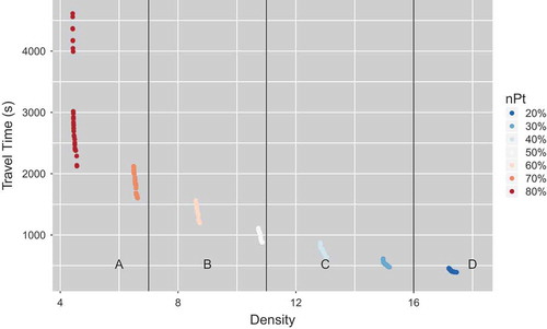
Figure 6 shows the hypervolumeof a typical run by both algorithms starting them with the same random seed. Figure 7 shows the sets of non-dominated solutions found by the algorithms for the same runs. Solutions by A$\epsilon S$ $\epsilon H$ are shown in black, whereas solutions by A$\epsilon$S$v$H are colored according to $n_{Pt}$ values. Note that A$\epsilon$S$v$H can find solutions for all proportions of public transportation users $n_{Pt}$, whereas A$\epsilon S$ $\epsilon H$ loses diversity in variable space and is not able to find solutions for large values of $n_{Pt}$, particularly for $0.7$ and $0.8$. In addition, note that for all values of $n_{Pt}$ solutions by A$\epsilon$S$v$H converge to better values in objective space than solutions by A$\epsilon S$ $\epsilon H$.

The two set coverage index is a metric used to compare non-dominated sets found by muti-objective EAs and expressed in Equation (8). Given two Pareto non-dominated sets, A and B, set-coverage C(A,B) counts the number of solutions in the set B that are dominated by the solutions in the set A upon the number of solutions in the set B.

(8) $C(A,B)=\frac{\left|\right\{b\in B|\exists a\in A:a\underset{-}{\prec }b\}|}{\left|B\right|}$(8)

Table 2 shows the average set-coverage values of the Pareto non-dominated solutions found by both algorithms. Note that in average solutions by A$\epsilon$S$v$H dominate many more solutions by A$\epsilon S$ $\epsilon H$, which is in accordance with the hypervolumevalues reported above.

Table 2. Two set coverage index (C)

	Mean	SD
C(A$\epsilon$S$\epsilon$H,A$\epsilon$S$v$H)	0.24	0.18
C(A$\epsilon$S$v$H,A$\epsilon$S$\epsilon$H)	0.50	0.31

In the following we focus our analysis on solutions found by A$\epsilon$S$v$H.

4.3. Trade-offs

Next, we analyze trade-offs between objectives. Unless stated otherwise, we use in our analysis the set of non-dominated solutions found in the 10 runs of the algorithm. The correlation values between objectives travel time (tt) and density (dens) are shown in Table 3, where negative correlations suggest trade-offs between objectives. This table also includes the correlation between the objectives and fuel consumption (fc), which is measured but not used for optimization.

Table 3. Objective correlation matrix

	tt	dens	fc
tt	—	−0.91	−0.92
dens	−0.91	—	0.99
fc	−0.92	0.99	—

Figure 8 shows the trade-off between travel time and density, which is in agreement with the negative correlation shown in Table 3. This figure is colored according to the proportion of agents $n_{Pt}$ that use public transportation. Also, it includes vertical lines to mark ranges of the LoS computed from the traffic density. To compute LoS, we use the six levels of service defined by The Highway Capacity Manual (Board, 2000), designated by the letters A through F, with A being the highest LoS and F the lowest. Table 4 shows the different levels according to density. In the figure, the lines correspond to ranges of LoS A–D.

Table 4. Levels of service for basic freeways segments

Levels of	Density
service	(pc/km/ln)
A	0–7
B	7–11
C	11–16
D	16–22
E	22–28
F	> 28

From this figure, it can be seen that high densities of traffic correspond to smaller proportions of public transportation users $n_{Pt}$ and vice versa, as expected. Regarding levels of service, note that the best LoS A requires that 70% and 80% of the agents use public transportation, LoS B can be achieved with 50% and 60% of these agents, level C with 30% and 40%, and the worst level D requires 20% when more people uses private cars that leads to the highest density of traffic.

From the same figure, we note that solutions for a given value of $n_{Pt}$ are clustered in density and travel time. An analysis of these clusters and their trade-off ranges provide valuable information. To illustrate, note that within each cluster there is no much difference in density, but travel time can change significantly, especially for larger fractions of public transportation users. The difference in travel time for each value of $n_{Pt}$ is due to the various configurations of bus headways and bus capacities. Within each cluster, solutions with lower travel time are achieved by scheduling large capacity buses with high frequency. As mentioned above, larger trade-off ranges in travel time are seen for larger $n_{Pt}$, where public transportation is used more. For example, the trade-off range in average travel time is around 500 s for cluster $n_{Pt}=70\mathrm{\%}$ and 150 s for cluster $n_{Pt}=30\mathrm{\%}$. This clearly shows ranges of improvement in travel time that can be achieved by optimizing public transportation with almost no impact to traffic density for a given value of $n_{Pt}$. On the other hand, notable changes in density are observed between clusters, for different values of $n_{Pt}$. This suggests that to reduce density a significant number of users should be encouraged to use public transportation instead of private cars.

In addition to travel time and density, we also estimate fuel consumption though at this time we do not use it as an objective value for optimization. Figure 9 shows travel time and fuel consumption, coloring solutions by the LoS. Note that there is a perceptible trade-off between fuel consumption and travel time, in agreement with the negative correlation shown in Table 3. Looking at the levels of service, note that in general solutions with the best LoS, such as A and B, have lower values of fuel consumption, but higher travel times. This is because high levels of service imply low traffic densities, and vice versa. High levels of service are achieved under scenarios with larger fractions of public transportation users, where, on average takes the user longer to get to their destinations, but less private vehicles circulate the city. On the other hand, solutions with worst levels of service, C and D, in general show better travel time but worse fuel consumption. Thus, the increase in fuel consumption is because more people use their cars instead of public transportation.

Figure 9. Fuel consumption and travel time, colored by level of service.

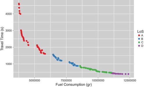
Figure 10. Fuel consumption and density, colored by fraction of public transport users ${\mathit{n}}_{\mathit{P}\mathit{t}}$.

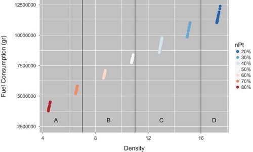
Figure 11. Trade-off TT and PM by ${\mathit{n}}_{\mathit{P}\mathit{t}}$.

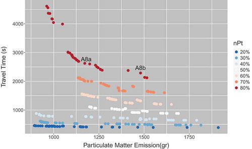
Figure 12. Number of public transportation trips by ${\mathit{n}}_{\mathit{P}\mathit{t}}$.

Due to the high positive correlation between density and fuel consumption, shown in Table 3, a clear correspondence between Fig. 8 and 9 emerges. Looking at these two figures, note that for a given fraction $n_{Pt}$ of public transportation users the difference in fuel consumption can become significant although density does not change much. This can be seen clearer in Figure 10 that shows fuel consumption and density, coloring solutions according to $n_{Pt}$. The strong positive correlation between density and fuel consumption suggests that the latter could be used instead of the former as objective value for optimization.

Figure 13. Public transportation PM emission by ${\mathit{n}}_{\mathit{P}\mathit{t}}$.

4.4. Emissions

Another important aspect of sustainable public transportation is its environmental impact. As stated above, larger fractions of public transportation users $n_{Pt}$ reduce overall fuel consumption in the city as shown in Figure 10. Also, best levels of service and low levels of fuel consumption can be achieved simultaneously, as shown in Figure 9.

In addition to fuel consumption, we collect data from MATSim’s emissions module. In this work, we analyze particulate matter (PM) emissions. The concentration of PM is composed of engine exhaust gas emissions as well as abrasion and suspension. Regarding health effects, the smaller the particle, the worse the impact on humans. The effects range from damages of the respiratory system to carcinogenic effects.

Figure 11 shows travel time against PM emissions of the non-dominated solutions found by the EA, coloring by $n_{Pt}$. Note that there is a trade-off between travel time and PM emissions within each cluster $n_{Pt}$. For a given fraction of $n_{Pt}$ the number of private cars is the same and the range of PM emissions observed is determined by the different configurations of headways (frequency) of buses. Thus, for a given $n_{Pt}$, increasing the frequency of buses reduces travel time but increases PM. The difference in travel time is more notorious for large $n_{Pt}$, where most people use public transportation. In this work we model buses with diesel as fuel, which reflects the current technology for most buses in Quito. This result suggests that a change of technology for buses, for example, from diesel to electric, is essential to achieve reasonable travel time and low traffic densities with minimum PM emissions.

Figure 11 shows that the upper bound of PM increases with smaller fractions of $n_{Pt}$. This is due to configurations with high frequency of buses combined with a large number of private cars. In fact, the solution with highest PM emissions for $n_{Pt}=80\mathrm{\%}$ includes a configuration where buses are run with slightly higher frequency than the solution with highest PM emissions for $n_{Pt}=30\mathrm{\%}$. Therefore, the difference in PM emissions between these two extreme solution is mostly due to the difference in the number of private cars. High-frequency configurations of buses for low demand scenarios slightly reduce travel time and are likely to have a lower occupancy rate. These solutions appear as non-dominated because at this time we do not consider cost nor take into account occupancy rate of the buses.

Figures 12 and 13 show box plots of the number of public transportation trips and PM emissions, respectively, grouped by $n_{Pt}$. From these figures, we note that the median of number of trips and PM emissions increase with $n_{Pt}$ from $20\mathrm{\%}$ to $50\mathrm{\%}$, and are similar for fractions $60\mathrm{\%}$ and above.

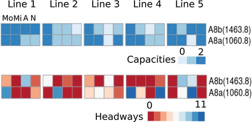
We analyze with more detail two solutions found by the algorithm for $n_{Pt}=80\mathrm{\%}$, denoted as A8b and A8a as shown on Figure 11. Note that there is a considerable difference in PM emissions between them. Figure 14 shows separately the configurations of bus capacities (top) and headways (bottom) of all five lines and schedules for these solutions. Capacities and headways are colored according to their code. Together to the identifier of the solution we also include the value of PM emissions computed for public transportation, which are lower than those reported in Figure 11 where the value of PM emissions include private cars as well. Note that overall the frequency of buses is higher in A8b than in A8a, which is reflected in the values of PM emissions. In addition, note that to satisfy the high demand of public transportation these solutions require low capacities and relatively low frequencies for some lines and schedules, see, for example, Line3 in the afternoon schedule. This illustrates the relevance of assigning buses of different capacities and frequencies to different schedules.

Figure 14. Configuration of bus capacities (top) and headways (bottom) of solutions A8b and A8a. Schedules: Mo, Mi, A, N (morning, midday, afternoon, night). Capacities: 0, 1, 2 (small, medium, large). Headways: 0,…, 11 (5 min, …, 60 min).

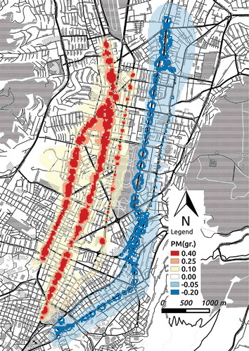
The geo-located differences in PM emissions between A8b and A8a are illustrated in Figure 15, where red color indicates an increase of PM emissions in A8b and blue a reduction. Note, for example, that the levels of PM increase considerably on the network segments where bus Lines 4 and 3 are located (see Figure 2 for the location of bus lines), where A8b has higher frequency than A8a as shown in Figure 14.

5. Conclusions and future work

This work studied levels of service in urban transportation on a scenario of a real-world traffic network. We coupled a multi-objective EA with the multi-agent transport simulator MATSim to perform a bi-level search of the proportions of private/public transportation users and optimal configurations of buses capacities and headways associated to each proportion. The multi-objective EA minimized travel time and density simultaneously. We defined levels of service in terms of density and analyzed it in conjunction with the trade-offs between objectives on the set of non-dominated solutions found in 10 runs of the algorithm. We also analyzed fuel consumption and the effects of PM emission over the area. The results of this study provide valuable insights to understand better the conditions that can lead to different levels of service in the city. It also suggests ways to improve mobility combining private and public transportation. Our results clearly show that to improve LoS, more travelers must use public transportation, but better LoS do not necessary implies a reduction in PM because it depends on the BRT headways and the diesel engines of the buses. Results also show that the trade-off between travel time and fuel consumption agree with several configurations in capacities and headways according to the proportion of users. Also, PM emission shows that some of that settings can be environmentally friendly and user convenient. That information is worthy for decision makers due to the compromise between that objectives. In addition, results suggest that a change of technology for buses is essential to achieve reasonable travel time and low traffic densities with minimum PM emissions.

In the future, we would like to refine the model to consider constraints in resources. Also, we include other objectives such as cost, waiting time, bus occupancy rates, and evaluate the impact of a transition towards hybrid and electrical cars for private and public transportation. We would also like to extend the definition of service to cover other criteria besides density.

Correction

This article was originally published with error. This version has been corrected/amended as follows: Funding statement has been updated to include Shinshu University (Japan) as one of the funders.

Additional information

Funding

This work was supported by Shinshu University (Japan) and the National Secretariat of Higher Education, Science, Technology and Innovation (Senescyt), Ecuador.

Notes on contributors

Rolando Armas

Rolando Armas has a PhD degree from the Interdisciplinary Graduate School of Science and Technology at Shinshu University, Nagano, Japan. His research interest includes sustainable systems, evolving design, evolutionary computation, traffic simulation, emission models, and data mining tools. Currently, he is a member of Frontiers in Massive Optimization and Computational Intelligence (MODO), an International Associated Laboratory between Japan and France which research includes massive optimization problems and massive optimization algorithms.

References

- Aguirre, H. , Yazawa, Y. , Oyama, A. , & Tanaka, K. (2014). Extending aeseh from many-objective to multi-objective optimization. In G. Dick , et al., (Eds.), Simulated evolution and learning . SEAL 2014. Lecture Notes in Computer Science, vol 8886. Springer, Cham.
- Aguirre, H. , Oyama, A. , & Tanaka, K. (2013). Adaptive ε-sampling and ε-hood for evolutionary many-objective optimization. In R. C. Purshouse, P. J. Fleming, C. M. Fonseca, S. Greco, & J. Shaw (eds.), Evolutionary multi-criterion optimization. EMO 2013. Lecture Notes in Computer Science, Vol. 7811. Springer Berlin Heidelberg.
- Arbex, R. O. , & da Cunha, C. B. (2015). Efficient transit network design and frequencies setting multiobjective optimization by alternating objective genetic algorithm. Transportation Research Part B: Methodological , 81, 355–376. doi:10.1016/j.trb.2015.06.014
- Bielli, M. , Caramia, M. , & Carotenuto, P. (2002). Genetic algorithms in bus network optimization. Transportation Research Part C: Emerging Technologies , 10(1), 19–34. doi:10.1016/S0968-090X(00)00048-6
- Board, T. R. (2000). Highway capacity manual (W. D. National Research Council, Ed.). Washington DC: National Research Council.
- Demoraes, F. (2005). Movilidad, elementos escenciales y riesgos en el distrito metropolitano de quito ( Unpublished doctoral dissertation). Universidad de Savoie, Francia.
- DMQ . (2012, March). Encuesta domiciliaria de movilidad (edm11) del distrito metropolitano de quito––13 de marzo de 2012 . (Presentation Document)
- DMQ . (2015, December). Empresa publica metropolitana de transporte de pasajeros––distrito metropolitano de quito rendicion de cuentas 2015 . (Document)
- Farhan, A. K. , Baldev, R. Marwah. , & Deb., Kalyanmoy , & Mohamed, R. K. (2005). A genetic algorithm based bus scheduling model for transit network . Proceedings of the eastern Asia society for transportation studies (Vol.5, pp. 477–489).
- Frederik, R. , Topf, J. , & Karch, C. (2007). Geofabrik. Retrieved January, 2014, from http://www.geofabrik.de
- Gakenheimer, R. (1999). Urban mobility in the developing world. Transportation Research Part A. Policy and Practice , 33, 671–689.
- GrupoFaro . (2010, March). Reverdeciendo las politicas: Hacia una movilidad sustentable en quito: El potencial de la bicicleta como medio de transporte alternativo. Retrieved January 2017, from http://www.grupofaro.org/
- Hee, K. J. , Kyung, B. Y. , & Hyuk, C. J. (2012). Multi objective optimization for sustainable road network design problem . International Conference on Transport, Environment and Civil Engineering (ICTECE’2012), August 25-26, 5, Kuala Lumpur.
- Horni, A. , Nagel, K. , & Axhausen, K. (2016). Multi-agent transport simulation MATSim . (L. U. Press., Ed.). London: Ubiquity Press. doi: 10.5334/baw.
- Hülsmann, F. , Gerike, R. , Benjamin, K. , Nagel, K. , & Luz, R. (2011). Towards a multi-agent based modeling approach for air pollutants in urban regions . Proceedings of the Conference on “Luftqualität an Straßen”, FGSV Verlag GmbH, 144–166. Retrieved from http://www.matsim.org/extension/emissions
- INEC . (2010). Ecuadorian national institute of statistics. Retrieved October, 2014 from http://www.ecuadorencifras.gob.ec/
- Keller, M. , & Wuthrich, P. (2014, June). Handbook emission factors for road transport 3.1/3.2 . Retrieved from http://www.hbefa.net/
- Ma, J. , Zhao, Y. , Yang, Y. , Liu, T. , Guan, W. , & Wang, J. (2017). A model for the stop planning and timetables of customized buses. In X. Ma, (ed.), PLoS ONE. 2017;12(1):e0168762. doi:10.1371/journal.pone.0168762.
- Roess, R. , Prassas, E. , & McShane, W. (2011). Traffic engineering (U. Ed. Pearson, Ed.) . USA: Ed.Pearson.
- United Nations, D. O. E. , & Social Affairs, P. D. (2014). World urbanization prospects: The 2014 revision .
- Verbas, Ä. Ö. , & Mahmassani, H. S. (2015). Integrated frequency allocation and user assignment in multimodal transit networks. Transportation Research Record: Journal of the Transportation Research Board , 2498, 37–45. doi:10.3141/2498-05
- Yu, B. , Yang, Z. , & Yao, J. (2010). Genetic algorithm for bus frequency optimization. Journal of Transportation Engineering , 136(6), 576–583. doi:10.1061/(ASCE)TE.1943-5436.0000119