A novel fuzzy energy based level set method for medical image segmentation

Abstract

Segmentation is a very important step in the field of image processing. Noise and intensity inhomogeneity make challenging the segmentation of images, especially for medical images. Fuzzy C-means (FCM) clustering is one of the most widely used methods in medical image segmentation, but it can not deal effectively with noise and intensity inhomogeneity. Accurate segmentation capability of level set-based active contour models make them attractive in medical image analysis but they also fail to perform better when medical images are corrupted by noise. To deal with Gaussian noise and intensity inhomogeneity, a new region-based level set model is proposed by integrating active contour and FCM clustering. In this method, FCM-based energy function is used with level set method to overcome local minimum problem of active contour modal. Distance Regularized Level Set Evolution (DRLSE) is used in proposed method to deal with re-initialization problem of traditional level set method. These two modifications in level set modal effectively deal with intensity inhomogeneity of medical image. A mean filter-like spatial term is also utilized with the proposed energy function, which makes this method advantageous for segmenting noisy images. The planned scheme is verified on diverse real medical images and synthetic images, which contain noise as well as intensity inhomogeneity. The proposed method is compared with other state-of-the-art methods in terms of Segmentation Accuracy, Precision, and Recall. Results show that the proposed method offers better performance compared to other latest methods for segmentation of noisy images.

Keywords:

• FCM
• level sets
• medical imaging
• segmentation

PUBLIC INTEREST STATEMENT

Image segmentation is the division of an image into its elements/regions and it is a very important aspect of medical image processing used for pathological diagnosis. Segmentation Accuracy is commonly used parameter for performance analysis of any techniques used for image segmentation. Intensity inhomogeneity and noise are the prime hurdles for precise segmentation of medical images. Proposed method deals efficiently with noise and intensity inhomogeneity of medical images.

1. Introduction

For medical images, active contour models are very efficient in distinguishing the boundaries. Active contours, referred as snakes, are the models which are used to extract the objects by making curves evolve by minimizing a defined energy. The energies used in these models are such that they are minimized when the curves evolve at the borders of the required object. Usually, these energies have two main components; internal energy and external energy. Internal energy makes the evolving curve smooth regularizing it, and external energy guides the motion of the curve toward its optimal position. The commonly used external energies are edge based (Caselles & Kimmel, 1997; Kichenassamy, Kumar, Olver, Tannenbaum, & Yezzi, 1995; Malladi, Sethian, & Vemuri, 1995) and region based (Chan & Vese, 2001; Li et al., 2011; Mumford & Shah, 1989; Vese & Chan, 2002). The active contour models make an automatic search for their minimum energy positions, but sometimes they may settle at a local minimum which makes them less effective. Integration of level sets approaches with edge-based active contour models and then applying them to image processing application was pioneered by Malladi et al. (1995). Until then, Snake models were implemented based on parameterized approaches which face a lot of complexities. Their proposed method includes an energy term based on edge information into a level set model which normally utilizes curvature motion. A similar approach based on level sets was proposed by Caselles, Catte, Coll, and Dibos (1993). After several years, Caselles and Kimmel (1997) propose one more approach based on edge information called as Geodesic Active Contours. A gradient flow-based model which is similar to Caselles and Kimmel (1997) was planned by Kichenassamy (1995) in the same year.

Mumford and Shah (1989) proposed a region-based approach to approximate an image using a piecewise smooth model of it. In this approach, energy term is minimized when the approximation contains smooth regions as well as a sufficient number of edges that can model the given image. The implementation approach for a particular solution of the Mumford–Shah model is given by Chan and Vese (2001). In this model, a piecewise constant approximation of an image is obtained instead of piecewise smooth. The required approximation of the image is achieved by using a level set model developed by Osher and Sethian (1988). The multiphase extension of (Chan & Vese, 2001) is proposed in (Vese & Chan, 2002) by Vese et al. In the recent years, many advance models are made based on the Chan and Vese (2001) model. One of such is proposed by C. Li et al. (2011) to overcome the intensity inhomogeneity. An energy function based on K-means clustering model is used in the suggested technique. The intensity is modeled using a multiplicative bias field term, and a local intensity clustering property is utilized to deal efficiently with inhomogeneity. Chen, Zhang, and Macione (2009) also suggested a method to deal with intensity inhomogeneity almost with the similar approach as in (Li et al., 2011) but using an additive bias field. The region-based model depends less on initial level set but edge-based models commonly suffer from the problem of level set initialization. B.N. Li, Chui, Chang, and Ong (2011) have used Fuzzy C-means (FCM) clustering’s membership function to initialize level set to overcome this problem. They also used the membership function to select the parameters required in the level set model. Cui, Wang, Fan, Feng, and Lei (2013) have utilized the local intensity clustering property in forming a new FCM-based clustering. L. Tang (2014) has utilized the concept of introducing fuzziness into the level set approach. They suggested an energy function by integrating FCM_S1&S2 model proposed by Chen and Zhang (2004) and level set model proposed by Samson, Blanc-F´eraud, Aubert, and Zerubia (2000). This model successfully segments out images with high noise, but most of the methods fail to perform better when medical images have noise and intensity inhomogeneity; so in proposed work, a novel fuzzy energy-based level set method along with Distance Regularized Level Set Evolution (DRLSC) and mean filter-based spatial term is proposed for medical image segmentation. The main contributions of the paper are as follows:

1. Proposed method effectively deals with intensity inhomogeneity of medical image using FCM-based energy function and DRLSC.

2. FCM membership function with multiplicative bias field term is used to overcome the problem of local minimum and DRLSC is used to deal with irregularities, developed due to re-initialization during level set evolution.

3. Proposed mean filter-based spatial term along with FCM-based energy function is used to minimize noise effect.

4. Proposed method provides superior segmentation results for medical images with intensity inhomogeneity as well as noise, and results are compared with other state-of-the-art methods in terms of Segmentation Accuracy (SA), Precision, and Recall.

The composition of the research paper is in this way. Section-2 of the research paper deals with background work in this field. The proposed method is discussed in section-3. Section-4 includes results/performance analysis with algorithm and implementation issues. Conclusion, which is followed by references, is explained in section-5.

2. Background

The proposed method is based on Mumford–Shah Model (1989) and Two-Phase Chan–Vese Model (2001) for image segmentation so these methods are explained in this section with the implementation of Chan–Vese Model for two-level Sets.

2.1. Mumford–Shah model

Mumford and Shah (1989) proposed a piecewise smooth model to segment the image, based on the following assumptions:

1. The image varies smoothly in the region

2. The image varies discontinuously across the boundaries between regions.

Let us assume that $I:\mathbf{\Omega }\to R$ is a gray-level image, where $\mathrm{\Omega }$ represents the image domain. Segmentation of the image is achieved by dividing $\mathbf{\Omega }$ into different regions $\left\{{\mathrm{\Omega }}_1,{\mathrm{\Omega }}_2,\dots ,{\mathrm{\Omega }}_N\right\}$, those are separated by a contour C and represented as:

(1) $\mathrm{\Omega }=U_i{\mathrm{\Omega }}_i\cup \hspace{0.17em}C$(1)

To achieve piecewise smooth approximation of the image I, the energy function proposed by Mumford–Shah model should be minimized, which is given by:

(2) $F^{MS}=\hspace{0.17em}\underset{\mathrm{\Omega }}{\overset{\hspace{0.17em}}{\int }}{\left(1-u\right)}^{2}dx+\mu \underset{\mathrm{\Omega }/\mathrm{C}}{\overset{\hspace{0.17em}}{\int }}\mathrm{\nabla }{u}^{2}dx+v|C|$(2)

where $\mu$and $v$ are fixed parameters. $u$ signifies the piecewise soft approximation of the observed image I. Value of $u$ is such that it contains smoothly varying values in a region $\mathrm{\Omega }$ and varies rapidly across the boundaries. The first and second terms in the above model ensure that $u$ follows the above-described properties of the image. The first term makes sure that $u$ is close to the image, I. Smoothness of $u$is controlled by the second term. Term $\left|C\right|$ gives the length of the curve to regularize the contour.

2.2. Two-phase Chan–Vese model

The implementation approach for Mumford–Shah (1989) model was proposed by Chan&Vese (2001) by taking a special case of the piecewise constant model, where the piecewise smooth model $u$is replaced by a piecewise constant approximation of it. In this case, energy function given by Equation (2) is represented like:

(3) $F^{MC}\left({\mathrm{\Omega }}_1,{\mathrm{\Omega }}_2\dots ..{\mathrm{\Omega }}_{\mathrm{N}}\right)=\sum _{i=1}^N\left\{\underset{{\mathrm{\Omega }}_i}{\overset{\hspace{0.17em}}{\int }}\hspace{0.17em}{\left(I-u_i\right)}^{2}dx+\hspace{0.17em}\underset{{\mathrm{\Omega }}_i}{\overset{\hspace{0.17em}}{\int }}\mathrm{\nabla }{u_i}^{2}dx+v|C_i|\right\}$(3)

For two-phase Chan–Vese model, two separate regions ${\mathrm{\Omega }}_1$ and ${\mathrm{\Omega }}_2$ in the image are achieved by minimization of abovementioned Chan–Vese model. Regions ${\mathrm{\Omega }}_1$ and ${\mathrm{\Omega }}_2$ are separated by a contour C and ${\mathrm{\Omega }}_1,{\mathrm{\Omega }}_2$ are inside and outside regions, respectively, with reference to contour C. It is assumed that the intensities inside these two regions are approximately constant. The fitting energy function used for this purpose is given by:

(4) $E\left(C\right)=E_1\left(C\right)+E_2\left(C\right)=\underset{{\mathrm{\Omega }}_1}{\overset{}{\int }}{\left(I-c_1\right)}^{2}dx+\underset{{\mathrm{\Omega }}_2}{\overset{}{\int }}{\left(I-c_2\right)}^{2}dx$(4)

where $c_1$ and $c_2$ represent the average intensity of an image in the regions ${\mathrm{\Omega }}_1,{\mathrm{\Omega }}_2$, respectively.

The fitting function has value as per contour C like:

$\text{E(C) = ,left{ matrix{ {Eleft({{C\_0}} right) = 0;{rm{ If }}C{rm{ is exactly at boundary}}} cr cr {{E\_1}left(C right) gt 0, {E\_2}left(C right) lt 0;{rm{If }}C{rm{ is inside of boundary}}} cr cr {{E\_1}left(C right) lt 0,{E\_2}left(C right) gt 0;{rm{If }}C{rm{ is outside of boundary}}}}}right.}$

By adding regularization terms to the fitting function given by Equation (4), energy function given by Chan&Vese becomes:

(5) $F\left(c_1,c_2,C\right)=\mu Length\left(C\right)+vArea\left(\mathrm{\Omega }\right)+{\lambda }_1\underset{{\mathrm{\Omega }}_1}{\overset{}{\int }}{\left(I-c_1\right)}^{2}dx+{\lambda }_2\underset{{\mathrm{\Omega }}_2}{\overset{}{\int }}{\left(I-c_2\right)}^{2}dx$(5)

where $\mu$ and $v$are constant parameters whose values can be positive or zero. Values of ${\lambda }_1,{\lambda }_2$ affect the weight given to the regions, most of the cases they are taken as unity. Length (C) is the length of curve/contour and Area (Ω) is the area of the image, I. This model will be equivalent to the Mumford–Shah model if $v=0,{\lambda }_1={\lambda }_2={\lambda }_{}$ and the constant approximations $c_1,c_2$ are replaced by piecewise smooth approximations.

2.3. Implementation of Chan–Vese model for two-level set

If curve/contour C is represented by zero-level set ${\varphi }_0\left(x\right)$ of level set function$\varphi \left(x\right):\mathbf{\Omega }\to R$, two-level sets function is defined (Osher & Sethian, 1988) as:

(6) $\varphi \left(x\right)=\left\{\begin{array}{c}x\in C;\varphi \left(x\right)=0\\ x\in {\mathrm{\Omega }}_1;\varphi \left(x\right)>0\\ x\in {\mathrm{\Omega }}_2;\varphi \left(x\right)<0\end{array}\right.$(6)

and Length (C) and Area (Ω) are given by:

(7) $Length\left(C\right)=Length\left\{\varphi =0\right\}=\underset{\mathrm{\Omega }}{\overset{}{\int }}\left|\mathrm{\nabla }H\left(\varphi \left(x\right)\right)\right|dx=\underset{\mathrm{\Omega }}{\overset{}{\int }}{\delta }_0\left(\varphi \left(x\right)\right)\left|\mathrm{\nabla }\varphi \left(x\right)\right|dx$(7)

(8) $Area\left(\mathrm{\Omega }\right)=Area\left(\varphi \ge 0\right)=\underset{\mathrm{\Omega }}{\overset{}{\int }}H\left(\varphi \left(x\right)\right)dx$(8)

where$H(\varphi \left(x\right)$ represents Heaviside function and ${\delta }_0\left(\varphi \left(x\right)\right)$ represents Dirac delta function. They are defined as:

(9) $H\left(z\right)=\left\{\begin{array}{c}1,ifz\ge 0\\ 0,ifz<0\end{array}\right.$(9)

(10) ${\delta }_0\left(z\right)=\frac{dH\left(z\right)}{dz}$(10)

The fitting energy terms for two-level sets function become:

(11) $E_1\left(C\right)=\underset{{\mathrm{\Omega }}_1}{\overset{}{\int }}{\left(I-c_1\right)}^{2}dx=\underset{\varphi >0}{\overset{}{\int }}{\left(I-c_1\right)}^{2}dx=\underset{\mathrm{\Omega }}{\overset{}{\int }}{\left(I-c_1\right)}^{2}H\left(\varphi \left(x\right)\right)dx$(11)

and

(12) $E_2\left(C\right)=\underset{{\mathrm{\Omega }}_2}{\overset{}{\int }}{\left(I-c_1\right)}^{2}dx=\underset{\varphi <0}{\overset{}{\int }}{\left(I-c_2\right)}^{2}dx=\underset{\mathrm{\Omega }}{\overset{}{\int }}{\left(I-c_2\right)}^2(1-H\left(\varphi \left(x\right)\right)dx$(12)

The Chan–Vese energy function for two level sets become:

$F^{cv}\left(c_1,c_2,C\right)=\mu \underset{\mathrm{\Omega }}{\overset{}{\int }}{\delta }_0\left(\varphi \left(x\right)\right)\left|\mathrm{\nabla }\varphi \left(x\right)\right|dx+v\underset{\mathrm{\Omega }}{\overset{}{\int }}H\left(\varphi \left(x\right)\right)dx+{\lambda }_1\underset{\mathrm{\Omega }}{\overset{}{\int }}{\left(I-c_1\right)}^{2}H\left(\varphi \left(x\right)\right)dx+{\lambda }_2\underset{\mathrm{\Omega }}{\overset{}{\int }}{\left(I-c_2\right)}^2(1-H\left(\varphi \left(x\right)\right)dx$

3. Proposed method

To deal with noise and intensity inhomogeneity of medical image, FCM-based energy function is used in the level set method to overcome the local minimum problem of active contour modal. Distance Regularized Level Set Evolution (DRLSE) is used in the proposed method to deal with the re-initialization problem of traditional level set method. These two modifications in level set modal effectively deal with intensity inhomogeneity of medical image by solving local minimum and re-initialization problems of active contour modal. A mean filter-like spatial term is also utilized with the proposed energy function to minimize noise effect, which makes this method advantageous for segmenting noisy images. Important characteristics of the proposed method are:

1. It is implemented using the level set method.

2. A fuzzy-based energy function is derived with consideration of region information and multiplied by a weight factor.

3. The intensity of the image is assumed to be modeled by original intensity multiplied by a biased field. The estimation of the biased field is carried out parallel to the evolution of level set using DRLSE, which makes it helpful to deal with inhomogeneity of medical image.

4. An improvement to membership of updating function is done by considering the spatial information and second update of membership values by using a spatial term, which results in de-noising of the medical image.

The workflow diagram of proposed method is depicted in Figure 1 as

Figure 1. Workflow diagram of proposed method.

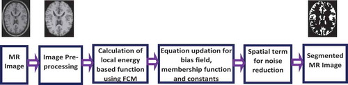
The proposed method is explained and implemented using following steps:

1. Image preprocessing

2. Calculation of local region-based energy function for image by using the FCM concept

3. Two-phase level set formulation

4. Multiphase level set formulation

5. Equations updation

6. Spatial term for reducing noise effect

3.1. Image preprocessing

Edge preserving filtering is used to preserve edge information in images. In the proposed research work, the median filter is used for edge-preserving smoothing of medical images. The median filter is a sliding-window spatial filter which replaces the center value with the median of all the pixel values in the window. Usually, the square kernel is used in case of the median filter but other shapes can be also used. A 3 × 3 window is used in proposed research work for edge-preserving smoothing of medical images.

3.2. Local region-based energy function

The Local region-based model is used to define energy function of proposed model by using the FCM concept. This fuzzy factor assigns each pixel to a particular region based on its membership function. For the medical image, this arrangement of pixel assignment is more suitable instead of hard assignment (Chen & Zhang, 2004) and this membership function is also utilized to decrease the result of noise. There are two purposes to be achieved using energy function, one is segmentation of image and other is to estimate the bias field. Real-world images can be modeled as a multiplicative field, added by noise. This can be represented as:

(14) $I=bJ+n$(14)

where$I$ is the observed image,$J$ is the true image, $b$ represents bias filed term, which represents intensity inhomogeneity, and $n$ is the additive noise. Salt and Pepper noise, Speckles noise, Blurred noise, Gaussian noise, and Poisson noise are commonly affected noises in medical images. Additive Gaussian noise with zero mean and constant variance is targeted in this research work. It is the most common type of noise in medical images results from the contributions of many independent signals (Gravel, Beaudoin, & De Guise, 2004).

The assumptions made in this model are:

1. The true image $J$ is assumed as a piecewise constant. i.e. in a given region ${\mathrm{\Omega }}_i$, it takes a constant value$c_i$.

2. Bias field$b$ varying very slowly which implies that in a small neighborhood, $b$ is constant.

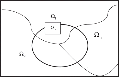
In given image, $I$ which is modeled using the Equation (14) and based on the above assumptions, the value of bias field, $b$ in a local neighborhood region is considered as constant. i.e. for a circular region,$O_y\subset \left\{x:|x-y|\le r\right\}$ of the image, shown in Figure 2, where $r$ represents the radius of circular region and $y\in \mathrm{\Omega }$, the value of bias field is:

Figure 2. Representation of local region O _y .

(15) $b\left(x\right)\approx b\left(y\right)forx\in O_y$(15)

By using Equations (14) and (15), intensity in the local region is modeled as:

(16) $I\left(x\right)=b\left(y\right)J\left(x\right)+n\left(x\right)forx\in O_y$(16)

By using the first postulation about$J(x)$, I(x) given by Equation (16) is expressed as:

(17) $I\left(x\right)=b\left(y\right)C_i+n\left(x\right)forx\in O_y\cap {\mathrm{\Omega }}_i$(17)

The additive Gaussian noise term can be eliminated if pixels in a region ${\mathrm{\Omega }}_i$, are considered to be part of a Gaussian distribution with mean $m_i=b\left(y\right)c_i$

The local region $O_y$ can be divided into N clusters, having centers at $m_i\approx b\left(y\right)c_i$, i varying from 1 to N. In this case, energy term of local region by using the FCM is given by:

(18) $F_y=\sum _{i=1}^N\underset{O_y\cap {\mathrm{\Omega }}_i}{\int }{u}_i^m\left(x\right){\left(I\left(x\right)-m_i\right)}^{2}dx$(18)

The fuzzy factor $m$decides the fuzziness and its value is normally taken as 2. In a local region $O_y$, center of the cluster $m_i$ can be replaced by$b\left(y\right)c_i$ and a window function is characterized as:

(19) $W\left(y-x\right)\subset \left\{W\left(y-x\right)=0,x\notin O_y\right\}$(19)

By using Equations (18) and (19) energy can be written in term of window function as:

(20) $F_y=\sum _{i=1}^N\underset{{\mathrm{\Omega }}_i}{\overset{}{\int }}{u}_i^m\left(x\right)W\left(y-x\right){\left(I-b\left(y\right)c_i\right)}^{2}dx$(20)

The overall energy by considering the total image domain $\mathrm{\Omega }$ is given by:

(21) $\text{Fleft({b,c,u,{{rm{Omega }}\_1},{{rm{Omega }}\_2} ldots {{rm{Omega }}\_N}} right) buildrel Delta over = {mathop int ^ ^}left{ {mathop sum limits\_{i = 1}^N ,,mathop int limits\_{{{rm{Omega }}\_i}}^{ } u\_i^{m}left(x right)Wleft({y - x} right), , {{left({I - bleft(y right){c\_i}} right)}^2}dx} right}dyquadquadquadquadquadquadquadquadquad,}$(21)

where c$=\left\{c_{1,}{c}_2\dots .c_N\right\}$ represents the constants. The selection of Kernel W is flexible. It should take null values outside the local region i.e. W (z) = 0 for $\left|z\right|>r$ and inside the region, it should have a sum of unity i.e. $\int W\left(z\right)=1$.

W (z) used in this model is:

(22) $W\left(z\right)=\left\{\begin{array}{c}\frac{1}{a}{e}^{-u^2/2{\sigma }^2},for\left|u\right|\le r\\ \\ 0,otherwise\end{array}\right.$(22)

Selection of the parameter a will depend on the value of σ (standard deviation) such that relation $\text{{mathop int nolimits{^} {^}}Wleft(z right) = 1}$ is satisfied. The selection of r is one of the crucial factors and the assumptions made on bias field are valid only when the neighborhood is small. The bias field varies faster so the value of r should be small.

3.3. Two-phase level set formulation

In the two-phase level set model of the proposed model, the image is divided into two regions ${\mathrm{\Omega }}_1$ and ${\mathrm{\Omega }}_2$ using a single-level set $\varphi$. The two regions are defined using the level set as:

1. In the region ${\mathrm{\Omega }}_1,M_1\left(\varphi \right)=H\left(\varphi \right)$

2. In ${\mathrm{\Omega }}_2,M_2\left(\varphi \right)=\left\{1-H\left(\varphi \right)\right\}$

Energy function is rewritten using these definitions and Equation (21) as:

(23) $\text{Fleft({b,c,u,phi } right) buildrel Delta over = {mathop int nolimits^ ^}left{ {mathop sum limits\_{i = 1}^2 {{mathop int nolimits^ }^}u\_i^{m}left(x right)Wleft({y - x} right){ }{{left({I - bleft(y right){c\_i}} right)}^2}{M\_i}left({phi left(x right)} right)dx} right}dyquadquadquadquadquadquadquadquadquadquadquad}$(23)

By exchanging order of integration, Equation (23) becomes:

(24) $\text{Fleft({b,c,u,phi } right) buildrel Delta over = {mathop int nolimits^ ^}mathop sum limits\_{i = 1}^2 u\_i^mleft(x right){ }{e\_i}left(x right){ }{M\_i}left({phi left(x right)} right)dxquadquadquadquadquadquadquadquadquadquadquadquadquadquadquadquadquadquadquadquadquad}$(24)

where $e_i(x)$ is defined as:

(25) $\text{{e\_i}left(x right) = { }{mathop int nolimits^ ^}Wleft({y - x} right){left({I - bleft(y right){c\_i}} right)^2}dyquadquadquadquadquadquadquadquadquadquadquadquadquadquadquadquadquadquadquadquadquadquadquad ,}$(25)

$e_i\left(x\right)$ can be rearranged in matrix form as:

(26) $e_i\left(x\right)=I^2{1}_K-2c_{i}I\left(b\ast K\right)+c_i^2\left(b^2\ast K\right)$(26)

where * represents the convolution and

(27) $\text{{1\_K} = { }{mathop int nolimits^ ^}Wleft({y - x} right)dy{ }quadquadquadquadquadquadquadquadquadquadquadquadquadquadquadquadquadquadquadquadquadquadquadquadquadquadquadquadquadquad }$(27)

The energy used for level set model is given by

(28) $F\left(b,c,u,\varphi \right)=-F\left(b,c,u,\varphi \right)+vL\left(\varphi \right)+\mu R_p\left(\varphi \right)$(28)

In this equation, $F\left(b,c,u,\varphi \right)$ is used as data term. $L\left(\varphi \right)$ and $R\left(\varphi \right)$ act as regularizing terms which are defined as:

(29) $L\left(\varphi \right)=\underset{\mathrm{\Omega }}{\overset{}{\int }}\left|\mathrm{\nabla }H\left(\varphi \right)\right|dx$(29)

and

(30) $\text{{R\_p}left(phi right) = {rm{ }}{mathop int nolimits^ ^}pnabla left(phi right)dxquadquadquadquadquadquadquadquadquadquadquadquadquadquadquadquadquadquadquadquadquadquadquadquadquadquadquadquadquadquadquad,}$(30)

$L\left(\varphi \right)$ represents length of contour or zero-level set of $\varphi$, which serves purpose of keeping the curve smooth by punishing length of it, and term $R_p\left(\varphi \right)$ is used to avoid re-initialization in level set evolution. Re-initialization is one of the disadvantages of the traditional level set model. During level set evolution, they develop irregularities and leads to numerical errors (Caselles & Kimmel, 1997). To overcome this, formal approach is to stop the evolution by using a signed distance function to redesign it. It is quite tricky to predict suitable time to apply re-initialization. To overcome this conflict, Li, Xu, Gui, and Fox (2010) planned a term called DRLSC. In level set functions signed, distance is maintained by this term. The gradient descent form for evolution of level set function is specified as

(31) $\frac{\mathrm{\partial }\varphi }{\mathrm{\partial }t}=-\frac{\mathrm{\partial }F}{\mathrm{\partial }\varphi }$(31)

when energy term $F\left(b,c,u,\varphi \right)$ is minimized with reference to $\varphi$(b, c as constants), Equation (31) results in

(32) $\frac{\mathrm{\partial }\varphi }{\mathrm{\partial }t}=\delta \left(\varphi \right)\left[(u_1^m{e}_1-u_2^m{e}_2\right)+vdiv\left\{\frac{\mathrm{\nabla }\varphi }{\left|\mathrm{\nabla }\varphi \right|}\right\}\mu div\left\{d_p\left(\left|\mathrm{\nabla }\varphi \right|\right)\mathrm{\nabla }\varphi \right\}$(32)

where

(33) $d_p\left(z\right)\stackrel{\mathrm{\Delta }}{=}\frac{p\left(s\right)}{s}$(33)

To achieve optimal solution using energy function along with level sets function, values of bias field b and constants c are also updated in a repetitive manner.

3.4. Multiphase level set formulation

The two-phase model can be extended to multiphase model, which is utilized for image segmentation using proposed energy function. In this case, k ≥ log₂N-level sets are required to solve the N-Phase problem. Ω can be divided into N regions, which are represented by $M_i\left\{{\varphi }_1\left(x\right),{\varphi }_2\left(x\right)\dots \dots \dots {\varphi }_k\left(x\right)\right\}$ and are defined as

(34) $\text{{M\_i}left{ {{phi \_1}left(x right),{phi \_2}left(x right) ldots ldots ldots {phi \_k}left(x right)} right} = left{ matrix{ {1,{ }if{ }x in { }{{rm{Omega }}\_i}{ }} cr {0,{ }Otherwise}}quadquadquadquadquadquadquadquadquadquadquadquadquadquadquadquadquad ,right.}$(34)

Energy function for multiphase is given by

(35) $\text{Fleft({b,c,u,phi } right) buildrel Delta over = {mathop int nolimits^ ^}mathop sum limits\_{i = 1}^N u\_i^mleft(x right){ }{e\_i}left(x right){ }{M\_i}left({phi left(x right)} right)dyquadquadquadquadquadquadquadquadquadquadquadquadquadquadquadquadquadquadquadquadquad}$(35)

where$\varphi =\left\{{\varphi }_1,{\varphi }_2\dots \dots \dots {\varphi }_k\right\}$ represents the level set vector.

The final energy function with regularizing terms is given by:

(36) $F\left(b,c,u,\varphi \right)=-F\left(b,c,u,\varphi \right)+v\sum _{i=1}^{k}L\left({\varphi }_i\right)+\mu \sum _{i=1}^k{R}_p\left({\varphi }_i\right)$(36)

The gradient descent equations are obtained by minimizing $F\left(b,c,u,\varphi \right)$ with respect to $\varphi$(b, c as constants) as:

(37) $\frac{\mathrm{\partial }{\varphi }_j}{\mathrm{\partial }t}=\sum _{i=1}^N\frac{\mathrm{\partial }{M}_i\left(\varphi \right)}{\mathrm{\partial }{\varphi }_j}{u}_i^m\left(x\right)e_i\left(x\right)+\delta ({\varphi }_j)vdiv\left\{\frac{\mathrm{\nabla }{\varphi }_j}{\left|\mathrm{\nabla }{\varphi }_j\right|}\right\}\mu div\left\{d_p\left(\left|\mathrm{\nabla }{\varphi }_j\right|\right)\mathrm{\nabla }{\varphi }_j\right\}$(37)

where j = 1, 2,………k

3.5. Equations updation

The updating equations for the bias field b, member ship function u, and constants c are obtained by minimizing $F\left(b,c,u,\varphi \right)$ with respect to b, u, or c by keeping other variables constant. To get the update equation for c, $F\left(b,c,u,\varphi \right)$ is minimized with reference to c by keeping $b,uand\varphi$ as constants. For derivative of $F\left(b,c,u,\varphi \right)$ with respect to $c_j$ by taking $b,uand\varphi$ as constant, all other terms of the summation in Equation (35) are independent of $c_j$, except the $j^{th}$ term so by putting derivative of $F\left(b,c,u,\varphi \right)$ equal to zero, following relation is obtained:

(38) $\text{{{partial Fleft({b,c,u,phi } right)} over {partial {c\_j}}} = { }{mathop int nolimits^ ^}u\_j^mleft(x right){{partial {e\_j}left(x right)} over {partial {c\_j}}}{M\_j}phi dx = 0quadquadquadquadquadquadquadquadquadquadquadquadquadquadquadquadquadquadquadquadquad}$(38)

And by taking derivative of $e_i\left(x\right)$ (given by Equation (25)) with respect to $c_j$ with taking $b,uand\varphi$ as constant:

(39) $\text{{{partial {e\_j}left(x right)} over {partial {c\_j}}} = - 2{mathop int nolimits^ ^}Wleft({y - x} right)left({Ileft(x right) - bleft(y right){c\_j}} right)bleft(y right)quadquadquadquadquadquadquadquadquadquadquadquadquadquadquadquadquadquadquadquadquad}$(39)

By using Equations (38) and (39):

(40) $\text{{{partial Fleft({b,c,u,phi } right)} over {partial {c\_j}}} = {mathop int nolimits^ ^}u\_j^mleft(x right){mathop int nolimits^ ^}Wleft({y - x} right)left({Ileft(x right) - bleft(y right){c\_j}} right)bleft(y right){M\_j}left(phi right)dx = 0quadquadquadquadquadquadquadquadquadquadquad}$(40)

or

(41) $\text{{mathop int nolimits^ }u\_j^mleft(x right)Ileft(x right){M\_j}left(phi right)left({{{mathop int nolimits^ }^}Wleft({y - x} right)bleft(y right)dy)} right)dx = {c\_j}{ }{mathop int nolimits^ ^}u\_j^mleft(x right){M\_j}left(phi right)({mathop int nolimits^ ^}Wleft({y - x} right){b^2}left(y right)dy)dx{ }quadquadquad }$(41)

so,

(42) $\text{{C\_j} = {{{{mathop int nolimits^ }^}left({b*W} right)I{M\_j}{ }left(phi right)dx} over {{{mathop int nolimits^ }^}left({b*W} right){M\_j}left(phi right)dx}}}$(42)

where $j=1,2\dots ..N$

The equation for bias field is updated by minimizing $F\left(b,c,u,\varphi \right)$ with respect to b by keeping $c,u,\varphi$ as constants. To minimize $F\left(b,c,u,\varphi \right)$, derivative of $F\left(b,c,u,\varphi \right)$(given by Equation (35)) with respect to b is set equal to zero, which results in the following relation:

(43) $\frac{\mathrm{\partial }F\left(b,c,u,\varphi \right)}{\mathrm{\partial }b\left(y\right)}=\sum _{i=1}^k\int u_i^m\left(x\right)\frac{\mathrm{\partial }{e}_i\left(x\right)}{\mathrm{\partial }b}{M}_i\left(\varphi \right)dx=0$(43)

And by taking derivative of $e_i\left(x\right)$ (given by Equation (25)) with respect to $b$ by taking $c,uand\varphi$ as constant:

(44) $\frac{\mathrm{\partial }{e}_i\left(x\right)}{\mathrm{\partial }b\left(y\right)}=-2W\left(y-x\right)\left(I\left(x\right)-b\left(y\right)c_i\right)c_i$(44)

By using Equations (43) and (44):

(45) $\frac{\mathrm{\partial }F\left(b,c,u,\varphi \right)}{\mathrm{\partial }b\left(y\right)}=\sum _{i=1}^k{u}_i^m\left(x\right)W\left(y-x\right)\left(I\left(x\right)-b\left(y\right)c_i\right)c_i{M}_i\left(\varphi \right)dx=0$(45)

or

(46) $\text{{int}Wleft({y - x} right)left{{ {mathop sum limits\_{i = 1}^k u\_i^{m}Ileft(x right){M\_i}left(phi right){c\_i}} right}dx = bleft(y right)left{{{{int }Wleft({y - x} right)(mathop sum limits\_{i = 1}^k u\_i^m{M\_i}left(phi right)c\_i^2)dx}} right}quadquadquadquadquadquadquad ,}$(46)

so

(47) $\hat{b}=\frac{\left(I{J}^{\left(1\right)}\right)\ast W}{\left(J^{\left(2\right)}\right)\ast W}$(47)

where

(48) $J^{\left(1\right)}=\sum _{i=1}^N{M}_i\left(\varphi \right)c_i{u}_i^m$(48)

and

(49) $J^{\left(2\right)}=\sum _{i=1}^N{M}_i\left(\varphi \right)c_i^2{u}_i^m$(49)

To get updating equation for $u_j$, energy term is solved using Lagrange multiplier as

(50) $F_m=F+\lambda \left\{1-\sum _{i=1}^k{u}_i^m\left(x\right)\right\}$(50)

and

(51) $\sum _{i=1}^m{u}_i^m\left(x\right)=1,\mathrm{\forall }x$(51)

These equations are updated by considering derivative of F_m with reference to $u_j$ (with $c,b,\varphi$ as constants) and equating it to zero. The estimated value of $u_j$ can be found as:

(52) $\frac{\mathrm{\partial }{F}_m}{\mathrm{\partial }{u}_j\left(x\right)}=m{u}_j^{m-1}\left(x\right)e_j\left(x\right)-\lambda =0$(52)

(53) $\Rightarrow \text{^}{u}_j={\left[\lambda /\left\{m{u}_j^{m-1}\left(x\right)e_j\left(x\right)\right\}\right]}^{\frac{1}{m-1}}$(53)

and

(54) $\sum _{i=1}^k{u}_i^m\left(x\right)=1,\mathrm{\forall }x$(54)

By using Equations (53) and (54):

(55) $\sum _{i=1}^k{\left[\lambda /\left\{m{u}_i^{m-1}\left(x\right)e_i\left(x\right)\right\}\right]}^{m/\left(m-1\right)}=1$(55)

so

(56) $\lambda ={\left[\sum _{i=1}^k{\left\{m{u}_i^{m-1}\left(x\right)e_i\left(x\right)\right\}}^{-1/\left(m-1\right)}\right]}^{-\left(m-1\right)}$(56)

By substituting value of $\lambda$ in Equation (53) gives:

(57) $\text{^}{u}_j=\frac{{\left\{u_j^{m-1}\left(x\right)e_j\left(x\right)\right\}}^{-1/\left(m-1\right)}}{{\sum }_{i=1}^k{\left\{u_i^{m-1}\left(x\right)e_i\left(x\right)\right\}}^{-1/\left(m-1\right)}}$(57)

3.6. Spatial term for reducing noise effect

A spatial term for fuzzy clustering using membership function is used in the level set formulation of the proposed method to subjugate noise effect. At every step along with bias filed, constants, and membership functions, the spatial term is also calculated. In the proposed method, spatial term is average of membership values of neighboring pixels and given as:

(58) $h_i\left(x\right)=\sum _{x_{r\in N_R\left(x\right)}}{u}_i\left(x_r\right)$(58)

By taking this extra spatial term into consideration, a pixel membership value is decided by the neighboring pixels. i.e. even if the center pixel is noisy, its effect can be truncated. Using this spatial term, the membership function is updated as:

(59) $\text{{u\_i}left(x right) = { }{{u\_i^{p}left(x right)h\_i^{q}left(x right)} over {sum nolimits{^k\_{j = 1}u\_j^{p}left(x right)h\_j^{q}left(x right)}}}$(59)

where p and q represent the weight given to each term. If noisy is heavy, more weight is given to the spatial term by considering large values for q. Median filter, Wiener filter, and Gaussian filter are also tested in the proposed method in place of mean filter-based spatial term. The median filter performs better for removing Salt and Pepper noise and Poisson noise, Wiener filter performs for removing Speckles noise and Gaussian filter for the Blurred noise. But in case of additive Gaussian noise with zero mean and constant variance, mean filter-based spatial term gives best results.

4. Results

The proposed method is verified with numerous synthetic images and real medical images, and results are compared with some of the states-of-the-art techniques. A CT scan image of the heart is taken from Cornell university database (www.via.cornell.edu/database) and MRI images are taken from database (www.humanconnectome.org) of Connectome Coordination Facility (CCF). Figure 3 displays corresponding results against evaluation of proposed method on a CT scan image of heart as:

Figure 3. Contour evaluation using different types of initialization.

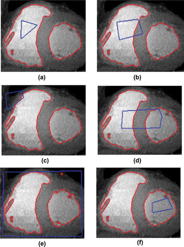
Initial contour in Figure 3(a) and Figure 3(f) is inside of the region of interest and in Figure 3(e), it is completely outside of the region. In all cases, the final contour is same and results are independent of initialization of initial contour. Here, proposed method is used without the spatial term. If the spatial term is also included in the proposed method, results are same since these images are without noise.

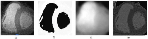
The original CT scan image, final segmented image, and bias field and corrected image using the bias filed are given in Figure 4 as:

Figure 4. (a) Original CT scan image (b) Final segmented image (c) Bias field (d) Corrected image using the bias filed.

In Figures 5–7, Brain MRI images obtained from web data set of CCF are used. The MRI data used are T1 normal MRI of 1 mm thickness with noise density of 9% and intensity non-uniformity of 40%.

Figure 5. Results of the proposed method and C. Li et al. (2011) on a noisy MRI image. (a, b) Bias field & final contour using Li’s method (c, d) Bias field & final contour using the proposed method.

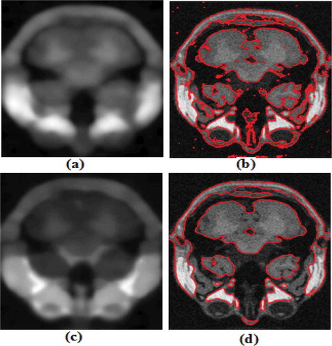
Figure 6. Results of the proposed method and B.N. Li et al. (2011) on a noisy MRI image. (a, b) Bias field & final contour using B.N Li’s method (c, d) Bias field & final contour using the proposed method.

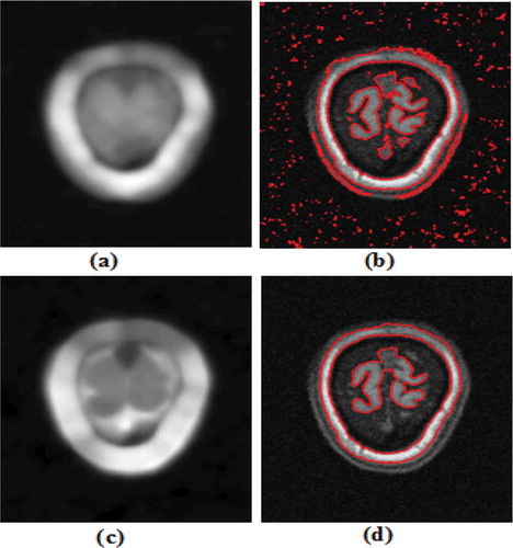
Figure 7. Results of the proposed method and W. Cui et al. (2013) on a noisy MRI image. (a, b) Bias field & final contour using W. Cui method (c, d) Bias field & final contour using the proposed method.

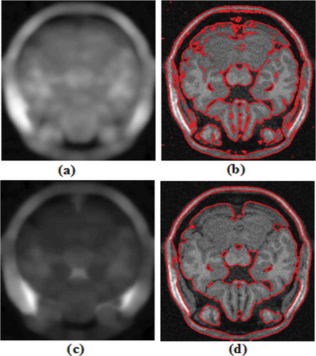
It can be observed from the images that final contour obtained by other methods is affected by the noise, and in case of the proposed method, the noise effect is either almost zero or very less. The proposed method gives superior results both in terms of bias field and final contour.

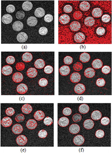
Results of the proposed method are compared with results of other methods for many synthesis images corrupted by different Gaussian noise (noise density,$\sigma =0to0.1$) and corresponding results of a synthesis image, added with Gaussian noise density (σ) of 0.02, are publicized in Figure 8.

Figure 8. (a) Noisy Image with Gaussian Noise Density of σ = 0.02. Results using (b) C. Li et al. (2011) (c) W. Cui et al. (2013) (d) Y. Chen et al. (2009) (e) B.N. Li et al. (2011) (f) proposed method.

The proposed method is compared with other latest methods on the basis of SA for same synthetic image corrupted by different Gaussian noise (noise density,$\sigma =0to0.1$). The values obtained by experimental evaluation are shown in Table 1. SA is defined as (Ahmed, Yamany, Mohamed, Farag, & Moriarty, 2002)

(60) $\mathrm{S}\mathrm{A}=\frac{\mathrm{N}\mathrm{u}\mathrm{m}\mathrm{b}\mathrm{e}\mathrm{r}\mathrm{o}\mathrm{f}\mathrm{C}\mathrm{o}\mathrm{r}\mathrm{r}\mathrm{e}\mathrm{c}\mathrm{t}\mathrm{l}\mathrm{y}\mathrm{C}\mathrm{l}\mathrm{a}\mathrm{s}\mathrm{s}\mathrm{i}\mathrm{f}\mathrm{i}\mathrm{e}\mathrm{d}\mathrm{P}\mathrm{i}\mathrm{x}\mathrm{e}\mathrm{l}\mathrm{s}}{\mathrm{T}\mathrm{o}\mathrm{t}\mathrm{a}\mathrm{l}\mathrm{N}\mathrm{u}\mathrm{m}\mathrm{b}\mathrm{e}\mathrm{r}\mathrm{o}\mathrm{f}\mathrm{P}\mathrm{i}\mathrm{x}\mathrm{e}\mathrm{l}\mathrm{s}}$(60)

Table 1. Segmentation Accuracy (SA) for synthetic image corrupted by Gaussian noise

Method	Noise Density
	0	0.02	0.04	0.06	0.08	0.10
C. Li et al. (2011)	92.81	88.26	86.18	83.65	78.95	76.56
W. Cui et al. (2013)	95.64	92.44	89.92	88.06	85.22	82.47
Y. Chen et al. (2009)	92.78	89.57	85.32	82.48	78.12	77.21
B.N. Li et al.(2011)	96.42	93.30	88.74	86.15	84.74	85.13
Proposed method	99.85	98.23	96.28	94.76	93.42	92.38

C. Li et al. (2011): A region-based method with K-means clustering-based energy function for image segmentation.

B.N. Li et al. (2011): A level set method with Fuzzy C-means (FCM) clustering’s membership function for image segmentation.

W. Cui et al. (2013): Localized FCM clustering with spatial information for medical image segmentation and bias field estimation.

Y. Chen et al. (2009): An improved level set method using additive bias field for brain MRI images segmentation.

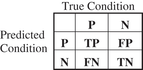
It can be observed that in case of segmentation of synthesis image, the proposed method has the minimum effect of noise compared to other methods. Precision and Recall curves are also commonly used for quantitative evaluation of image segmentation methods. In case of classification, Precision and Recall are referred as Positive Predictive Value (PPV) and True Positive Rate (TPR) or sensitivity, respectively. Precision and Recall are defined as

(61) $\mathrm{P}\mathrm{r}\mathrm{e}\mathrm{c}\mathrm{i}\mathrm{s}\mathrm{i}\mathrm{o}\mathrm{n}=\frac{\mathrm{T}\mathrm{P}}{\left(\mathrm{T}\mathrm{P}+\mathrm{F}\mathrm{P}\right)}$(61)

(62) $\mathrm{R}\mathrm{e}\mathrm{c}\mathrm{a}\mathrm{l}\mathrm{l}=\frac{\mathrm{T}\mathrm{P}}{\left(\mathrm{T}\mathrm{P}+\mathrm{F}\mathrm{N}\right)}$(62)

where $TP$,$FP$, TN and $FN$ are True Positive, False Positive, True Negative and False Negative, respectively, as per Figure 9 (Confusion Matrix)

Figure 9. Confusion matrix.

Precision and Recall curves of the proposed method along with state-of-the-art methods are plotted in Figure 10 for synthesis image corrupted with Gaussian noise (σ) of 0.02.

Figure 10. Precision and Recall curves for synthesis image with Gaussian noise density of 0.02.

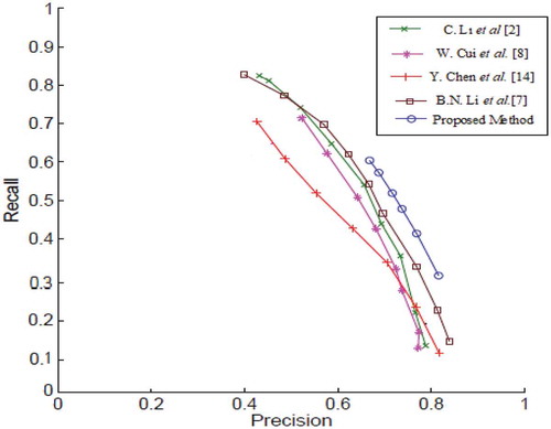
The Precision and Recall curves also verify that proposed method produces better segmentation. Larger Recall and Precision values in case of other methods come at the cost of undesirable over segmentation or under segmentation.

The proposed method is verified with different types of medical images like CT scan images of heart and brain MRI images. The results show that proposed method efficiently deals with noise as well as intensity inhomogeneity problem of synthesis and real-time medical images.

5. Conclusion

Results show that, in the proposed method, contour evaluation results are independent of the initialization of initial contour and final contour obtained by the proposed method is less affected by noise in comparison to other methods. Proposed method results in smooth contour even in existence of noise and non-uniformity. When the proposed method is compared with other methods in terms of SA of synthesis image corrupted by Gaussian Noise along with Precision and Recall curves, it shows better results. Median filter, Wiener filter, and Gaussian filter are also tested in the proposed method in place of mean filter-based spatial term. In case of additive Gaussian noise with zero mean and constant variance, mean filter-based spatial term gives best results. The proposed method has the better segmentation of medical images corrupted by both intensity inhomogeneity as well as noise, so proposed method can be utilized for medical applications, where high quality and precise segmentation are required. The proposed method is computationally complex since multiple similar convolutions are used repeatedly. As a future work, complexity can be reduced by using different types of level set methods for implementation of active contours and energy function using different FCM variations Choudhry and Kapoor (2016).

Acknowledgements

The authors thank Dr. Dinesh Kumar Vishwakarma for his valuable comments and support. http://www.dtu.ac.in/Web/Departments/Electronics/faculty/dkvishwakarma.php

Additional information

Funding

Not received any funding for this research.

Notes on contributors

Mahipal Singh Choudhry

Sh Mahipal Singh Choudhry is an Associate Professor in Department of Electronics & Communication Engineering, Delhi Technological University, India. He received both Bachelor and Master degrees in the field of Electronics & Communication Engineering from Malviya Regional Engineering College, now Malviya National Institute of Technology, India. His area of interest includes digital image processing and biomedical signal processing.

Rajiv Kapoor

Professor Rajiv Kapoor is Professor at Department of Electronics & Communication Engineering, Delhi Technological University, Delhi, India. Presently he is working as Principal at Ambedkar Institute of Advanced Communication Technologies & Research, Delhi, India. His areas of interest includes Signal Processing, Image Processing, Computer Vision and Robotics.

References

- Ahmed, M. N. , Yamany, S. M. , Mohamed, N. , Farag, A. A. , & Moriarty, T. (2002). A modified Fuzzy C-means algorithm for bias field estimation and segmentation of MRI data. IEEE Transactions on Medical Imaging , 21(3). doi:10.1109/42.996338
- Caselles, V. , Catte, F. , Coll, T. , & Dibos, F. (1993). A geometric model for active contours in image processing. Numerical Mathematical , 66(1), 1–31. doi:10.1007/BF01385685
- Caselles, V. , & Kimmel, R. (1997). Geodesic active contours. International Journal of Computer Vision , 22(1), 61–79. doi:10.1023/A:1007979827043
- Chan, T. , & Vese, L. (2001). Active contours without edges. IEEE Transactions on Image Processing , 10(2), 266–277. doi:10.1109/83.902291
- Chen, S. , & Zhang, D. (2004). Robust image segmentation using FCM with spatial constraints based on new kernel-induced distance measure. IEEE Transaction on System, Man and Cybernetics—Part B: Cybernetics , 34(4). doi:10.1109/TSMCB.2004.831165
- Chen, Y. , Zhang, J. , & Macione, J. (2009). An improved level set method for brain MR images segmentation and bias correction. Computerized Medical Imaging and Graphics , 33(7), 510–519. doi:10.1016/j.compmedimag.2009.04.009
- Choudhry, M. S. , & Kapoor, R. (2016). Performance analysis of Fuzzy C-means clustering methods for MR image segmentation. Procedia Computer Science , 89, 749–758. doi:10.1016/j.proces.2016.06.052
- Cui, W. , Wang, Y. , Fan, Y. , Feng, Y. , & Lei, T. (2013). Localized FCM clustering with spatial information for medical image segmentation and bias field estimation. International Journal of Biomedical Imaging , 2013, 1–8. Article ID 930301. doi:10.1155/2013/930301
- Gravel, P. , Beaudoin, G. , & De Guise, J. A. (2004). A method for modeling noise in medical images. IEEE Transactions on Medical Imaging , 23(10). doi:10.1109/10.1109
- Kichenassamy, S. , Kumar, A. , Olver, P. , Tannenbaum, A. , & Yezzi, A. (1995). Gradient flows and geometric active contour models. Proceeding, 5th International Conference Computer Vision , 810–815. doi:10.1109/ICCV.1995.466855
- Li, B. N. , Chui, C. , Chang, S. , & Ong, S. H. (2011). Integrating spatial fuzzy clustering with level set methods for automated medical image segmentation. Computers in Biology and Medicine , 41(1), 1–10. doi:10.1016/j.compbiomed.2010.10.007
- Li, C. , Huang, R. , Ding, Z. , Gatenby, J. C. , Metaxas, D. N. , & Gore, J. C. (2011). A level set method for image segmentation in the presence of intensity inhomogeneities with application to MRI. IEEE Transactions on Image Processing , 20(7). doi:10.1109/TIP.2011.2146190
- Li, C. , Xu, C. , Gui, C. , & Fox, M. D. (2010). Distance regularized level set evolution and its application to image segmentation. IEEE Transactions on Image Processing , 19, 12. doi:10.1109/TIP.2010.2069690
- Malladi, R. , Sethian, J. A. , & Vemuri, B. C. (1995). Shape modeling with front propagation: A level set approach. IEEE Transactions on Pattern Analysis and Machine Intelligence , 17(2), 158–175. doi:10.1109/34.368173
- Mumford, D. , & Shah, J. (1989). Optimal approximations by piecewise smooth functions and associated variational problems. Communications on Pure and Applied Mathematics , XLII, 577–685. doi:10.1002/cpa.3160420503
- Osher, S. , & Sethian, J. (1988). Fronts propagating with curvature-dependent speed: Algorithms based on Hamilton-Jacobi formulations. Journal of Computational Physics , 79(1), 12–49. doi:10.1016/0021-9991(88)90002-2
- Samson, C. , Blanc-F´eraud, L. , Aubert, G. , & Zerubia, J. (2000). Level set modal for image classification. International Journal of Computer Vision , 40(3), 187–197. doi:10.1023/A:1008183109594
- Tang, L. (2014). A variational level set model combined with FCMS for image clustering segmentation. Mathematical Problems in Engineering , 2014, 1–24. Article ID 145780. doi:10.1155/2014/145780
- Vese, L. A. , & Chan, T. F. (2002). A multiphase level set framework for image segmentation using the Mumford and Shah model. International Journal of Computer Vision , 40(3), 271–293. doi:10.1023/A:1020874308076